Flow of autonomous traffic on a single multi-lane street

Abstract

We investigate the behaviour of an original traffic model. The model considers a single multi-lane street, populated by autonomous vehicles directed from either end to the other. Lanes have no intrinsic directionality, and the vehicles are inserted at random at either end and any lane. Collision avoidance is fully automatic and, to enhance the transport capacity of the street, vehicles form trains in which they may travel at high speed quite close to the vehicle in front.

We report on the transit times for vehicles under a wide variety of conditions: vehicle insertion probability & imbalance and their maximum speed distribution. We also outline an interesting feature of the model, that the complex interactions of many vehicles are considerably more powerful than a simple ”keep left” directive which each vehicle should obey.

Motivations

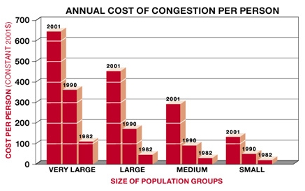
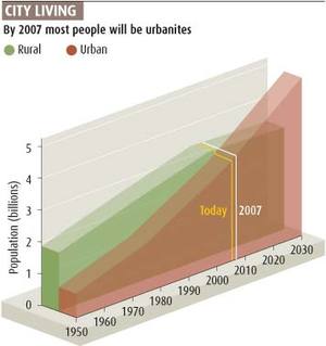
The worldwide transport infrastructure is becoming overloaded. In urban settings there is simply insufficient available real estate with which to increase capacity leading to increased commuting times and costs across all cities [1]. Figure 1 indicates how the cost of transport has increased in the last 25 years (in constant 2001 US$). It has been forecast that by this year, half the world’s population will live in urban areas (figure 2). Gridlock has become such an extensive problem that London city has introduced a heavy congestion charge for access to the city centre, though its effects are disputed [9]. Today’s cars are consuming resources at an ever-increasing rate and, despite the ubiquitous warnings of climate change associated with non-renewable energy consumption (the debate is still open, but the messages are certainly very present) [10], it seems that personal transport is not yielding.

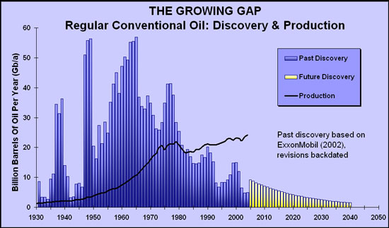
Today’s transport is completely dependent on a steady, secure and cheap supply of oil; this is difficult to guarantee for the future due to political instability and potentially limited resources (see figure 3). Indeed, some experts have stated that the era of cheap oil is drawing to a close [8] (though opinion is very divided) and that soon the world will have to turn to intrinsically difficult and expensive oil-extraction methods (shale oil, etc). The socio-economic implications are extremely profound and potentially dire.

Even renewable energy sources do not come close to solving the problem; a drastic worldwide push started today to develop renewable energy sources might already be too late to substitute oil before the economic consequences of a restricted oil supply would be felt and it is not clear that renewable energy could ever satisfy demand.

Safety and security in transport is also a continuing problem. The number of deaths on our roads is increasing as cars become faster - ironically, increased safety for the occupants implies a reduced safety for those outside. Driver frustration with congestion is also playing a part in agressive driving.

Thus, it is becoming clear that current trends are environmentally, economically and socially unsustainable in the long term. A paradigm-shift is required to break the current trend and give a new face to transport.

Proposed Model

In this article we report on the results of a first ’stepping stone’ to a complete computer model of a fleet of autonomous transport units. The overall image is of a transport infrastructure consisting of existing roads (implanted with RFID transponders), elevated or surface monorails and (possibly) a network of interconnected subsurface tunnels. Vehicles are completely self-controlled by on-board computers [4], other than to respond to a human initiated ”summons” and direct human input specifying the desired destination. Nearby vehicles travelling on the infrastructure maintain peer-to-peer [6] contact and share information [7] regarding traffic and viability, thus permitting real-time unsupervised route planning and execution.

Such a futuristic transport architecture would offer many long term benefits:

• Safer: Fully automated vehicles (no ”human error”); electronic response times to sudden dangers.

• Smarter: Advanced satellite navigation and information systems; ”intelligent” global response to perturbations.

• Sustainable: Efficient engines ”of the future”; solar panels could effectively provide a city with a 500MW power-station.

• Decongested: Real time propagation of traffic information and dynamic re-routing.

• Impartial: Suitable for all categories of end-user including transportation of goods.

• Greener: Energy source can be chosen by governments, be that oil, gas, nuclear or renewable; and would allow for centralised control over pollution.

Naturally any eventual implemetation of a system such as this would be long and difficult, requiring many phases of integration with the present transport infrastructure. We do not presently consider such problems, but only study how such a system might ultimately behave after all other conflicting forms of transport are rendered obsolete. We note, however, that present day vehicles could potentially be adapted for continued service.

As a typical city would consist of some $10^{5}-10^{6}$ vehicles, it will be necessary to understand precisely the interactions between them. Indeed, we can assume a priori that the system will self-organise itself to some attractor, which may or may not be a desirable final state, from the point of view of the end-user. The final emergent behaviour is likely to be complex in nature, bearing little or no similarity to the original rules under which each vehicle proceeds. Indeed, the scope of this research is to establish a phase diagram for the system; how the system globally behaves for given rule-sets applied to each vehicle. It is our intention to study the transport, navigation, routing and communications algorithms and infrastructure.

Heavy traffic in one direction will cause a street to be principally used by vehicles travelling in that direction. The real-time peer-to-peer propogation of information will allow other vehicles travelling in the opposite direction to adjust their routes accordingly.

Details of the model

The model discussed in this paper consists of a single multi-lane street, which is the first element of a larger simulation which will eventually encompass a small city. Lanes have no intrinsic directionality and vehicles are inserted at either end and any lane at random, subject to that lane being unoccupied in the vicinity of the entrance. All vehicles behave identically within their parameter specifications.

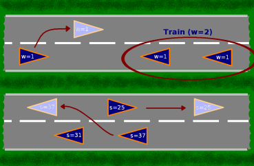
A central concept to this model is that of the weight of a vehicle, with a default value of unity. ”Heavier” vehicles may claim right-of-way over less heavy vehicles. In order to resolve conficts between vehicles of equal weight, each weight is adjusted by a small random value. Vehicles travelling in the same direction may form trains by summing their weights, and so obtain more right-of-way from oncoming vehicles in the same lane.

As oncoming vehicles much somehow pass one another, even on single lane streets, the ruleset assumes that any vehicle which comes to a halt also accosts itself to one side, and no longer blocks the lane.

All vehicles have a ”sensor” which collects all necessary information about other vehicles in the vicinity. The range of this ”sensor” is a parameter to the program, though we have observed that it has little effect except when decreased below the vehicles’ typical safe stopping distance.

Figure 4 illustrates two of the rules which vehicles obey. Given that each vehicle ”knows” exactly how all other vehicles behave, collision avoidance is simply a matter of having compatible rules for all vehicles involved in any interaction. Once this basic requirement is satisfied, one may move to study the properties of the model.

Results

The simulations we have run to date on the model have revealed that there is much work to be done. Even the few parameters specifying the model permit a very large variation in subsequent behaviour. We outline some aspects of this behaviour here. For all results reported below, we have fixed the number of lanes at 4, the length of the road at 2500 m, and, except where specified, the maximum velocity of each vehicle is a random number uniformly distributed from 10 to 30 m/s.

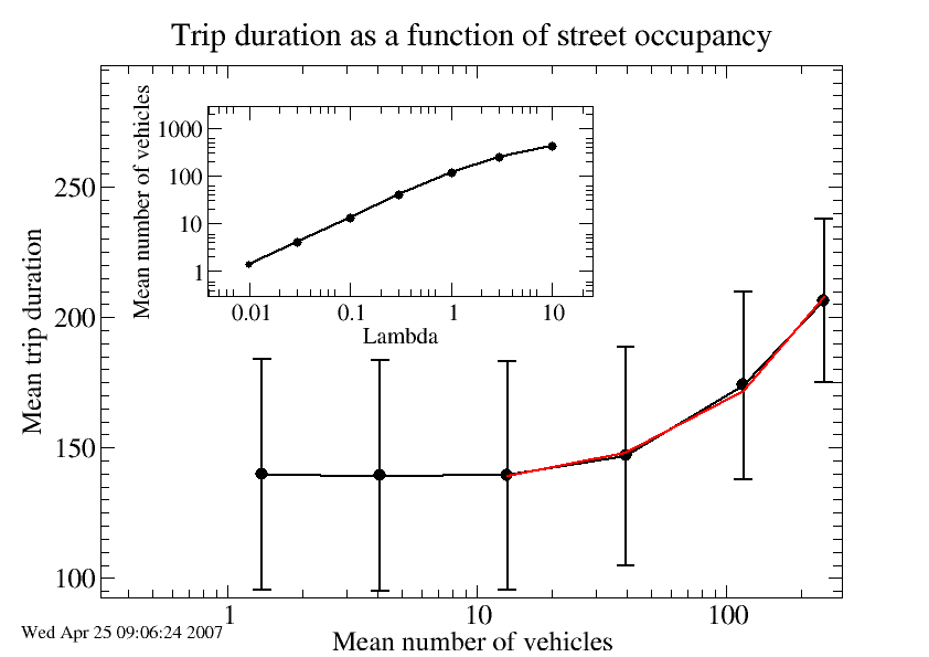
Figure 5 shows the variation of the average journey time as a function of the mean number of vehicles $N_{v}$ on the street. This parameter is altered by adjusting $\lambda$ the probability per unit time with which the system seeks to insert a new vehicle in each timestep. From the inset it is clear that when $\lambda\simeq 0$, $N_{v}\propto\lambda$. As $lambda$ increases, the entrance points to the street saturate and additional vehicles find it difficult to enter. The main figure instead demonstrates that the mean journey time remains constant for $N_{v}\to 0$, but, as the street begins to fill and vehicles find themselves impeded by those in front, the journey time increases approximately linearly with $N_{v}$.

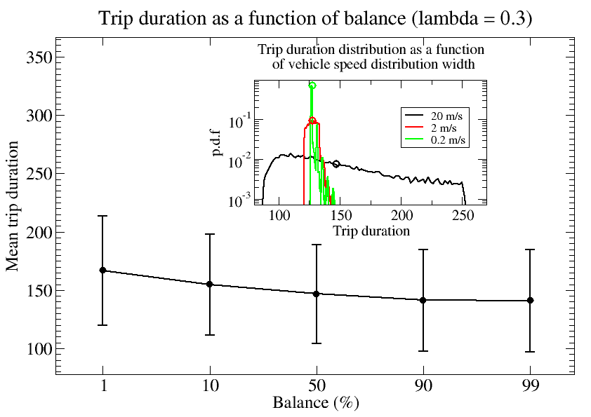
We have adapted the simulation to allow for unbalanced traffic, when vehicles arrive predominantly from one end or the other of the street. Figure 6 shows the mean journey time for cars entering from the left as a function of the percentage of total cars they represent (i.e. 1% implies most cars came from the right, 99% implies from the left). This was performed at $\lambda=0.3$ (at the point where vehicle interaction begins to impact on transit time) and it is clear that passively imposing a directionality on the street in this manner improves the journey time for those travelling with the main flow but penalises those travelling against. The inset to this figure demonstrates how the transit time varies with the homogeneity of the vehicles (at $\lambda=0.3$). When the width of the uniform distribution from which vehicle speeds are drawn is reduced from 20 to 0.2 m/s, while maintaining a mean of 20 m/s, the transit time distribution narrows almost to a delta, and reduces it’s mean by some 15%.

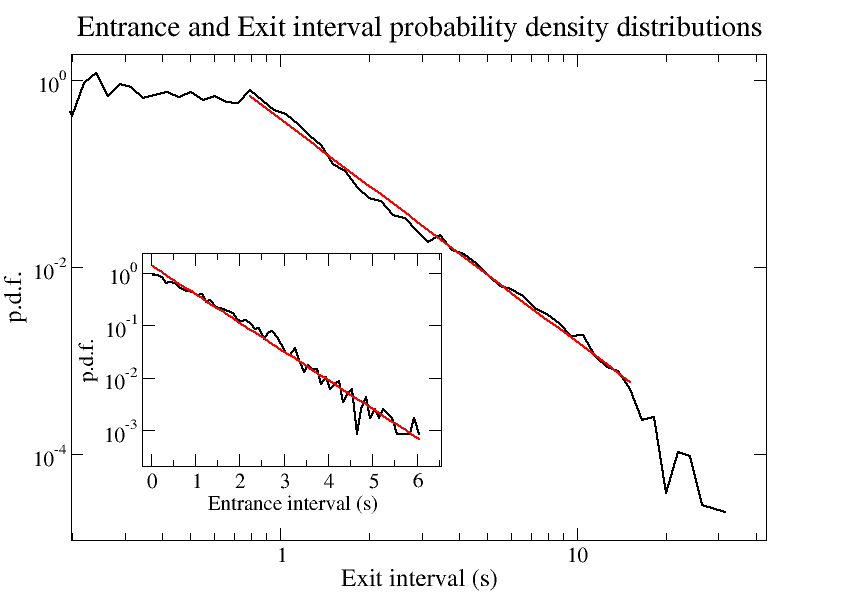
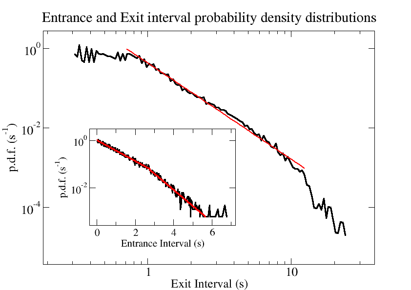
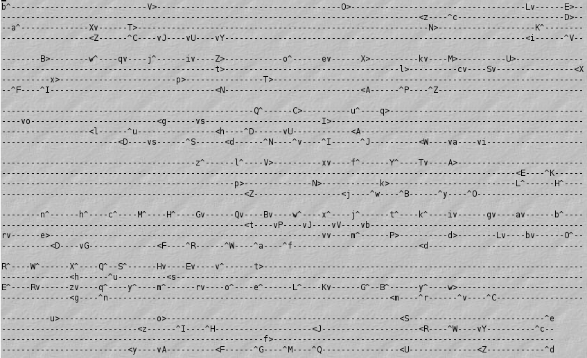
We now consider the processes of vehicles entering and exiting the street. As the vehicles enter with a given probability in each timestep, we expect this to be a Poisson process, with an exponentially improbable interval between the insertion of two subsequent vehicles. The inset for figure 7 demonstrates indeed that this is the case, while the main figure shows the same distribution for the exit process. Curiously the exit interval follows a power law from 1 to 10 seconds after which it decays rapidly. This suggests that vehicles are clustering in the street, and indeed, the screenshot shown in appendix 12 clearly indicates that this is so. That vehicles should exit with a power-law distribution of exit intervals is not desirable from a transport point of view, so it will be interesting to see how this feature behaves when many streets are modelled together. Figure 8 shows the same distributions for the ”keep left” model; diuscussed below.

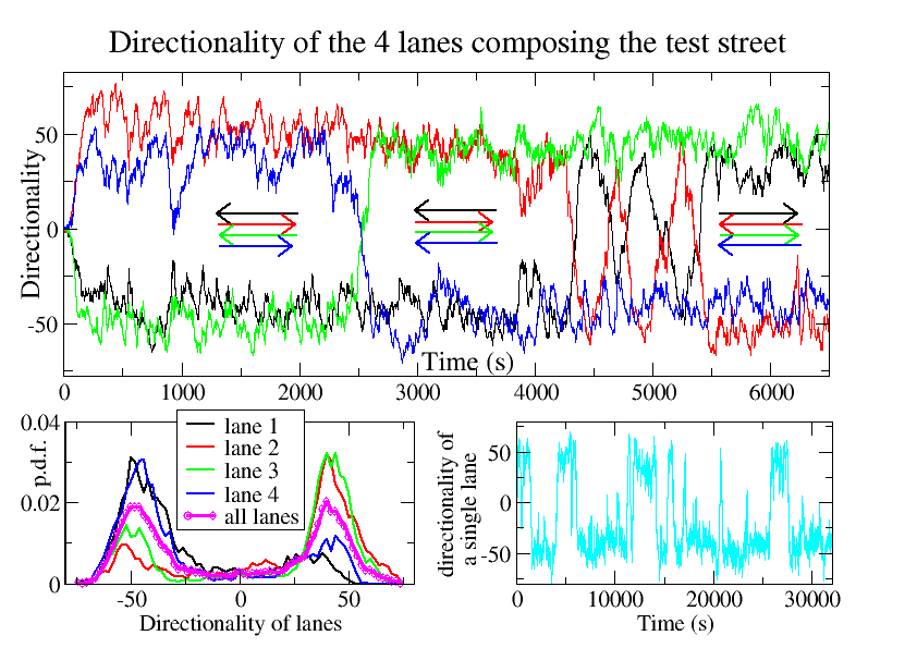
As the simulations presented here all specify a street with 4 lanes, we thought it interesting to see how the lanes are utilised by the vehicles. Our objective in this preliminary paper is to verify if vehicles can be made to form ”trains” with a minimum of rules, and so efficiently utilise the infrastructure available. To visualise how the lanes are being utilised, we assign a ”direction” to each lane which is equal to the number of vehicles moving in the positive direction minus the number moving in the negative direction, in that lane.

Figure 9 demonstrates that lanes do passively acquire a directionality. The main graph shows the direction of each lane as a function of time - it may be seen that lanes 2 and 4 immediately established a stable positive direction and 1 and 3 negative. After some time, lanes 3 and 4 exchange directions, and so on. The bottom left graph shows the probability distribution of each lane having a given direction. Though lanes may swap from positive to negative and vice-versa, evidently they always remain ”polarised”. The bottom right graph shows the directionality of a single lane as a function of time, discussed below.

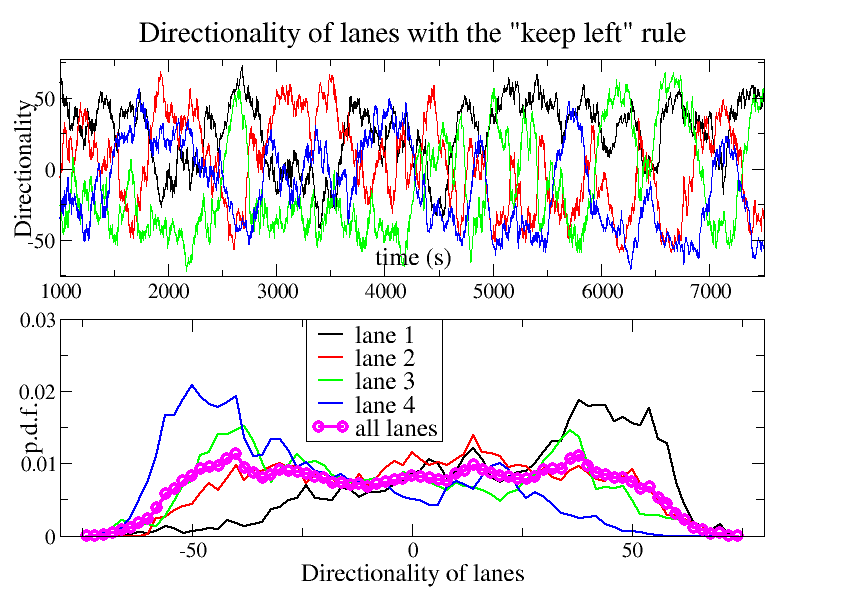
Considering figure 9 one may observe that adjacent lanes frequently acquire opposite directions. Upon reflection, we considered that this reduces efficiency, as faster vehicles will find it difficult to change to a different lane in order to pass slower vehicles. We have therefore implemented a ”keep left” rule in which, whenever a vehicle is required to change lane, it automatically seeks first to move to its left, choosing the right only if the left is not available. Furthermore, a vehicle proceeding normally will always seek to move to its left if possible. Naturally, our expectation was that lanes 1 and 2 would acquire a stable positive direction, with lanes 3 and 4 negative.

Figure 10 indicates however, that this does not occur. In fact, the ”keep left” rule clearly has an undesirable effect: lanes lose much of their directionality, and change from positive to negative considerably more frequently. The ”keep left” rule did not cause vehicles to keep very much to the left! This is a very simple example of the complexity inherent to the problem: though individual, isolated vehicles will stay on the left, many interacting vehicles do not.

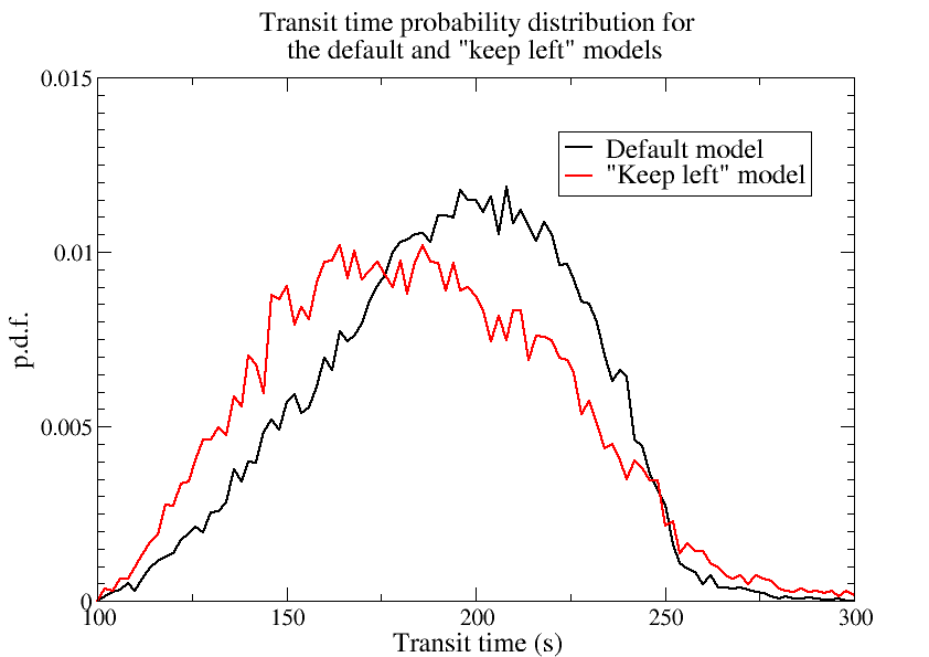
Strangely, however, the keep left rule does in fact improve the overall efficiency. Mean transit time for all vehicles improves from 195 to 185 seconds, though the width of the distribution increases by appx. 6 seconds and the tail seems longer. Figure 11 shows a comparison between the duration distrubtions for two realisations, one with the ”keep left” rule, one without. This distribution do not seem to follow any particular form, though we have observed that it is highly dependent on the ruleset. Figure 8 shows the entrance and exit interval distributions for the ”keep left” model; they do not significantly change with respect to the default, though it seems that the Poisson entrance process is somewhat modified - it may be that vehicles clustering on the left near the entrance is the cause. It yet remains to be verified if the ”keep left” rule actually confers a net advantage or not.

This article represents the first results in what is planned to be a much more comprehensive simulation of an autonomous transport system. As such, it is very much exploratory and the meaning of these first observations have yet to be defined and categorised in accordance with existing research.

Nonetheless, we note some interesting points. That the exit process follows a power-law distribution of intervals suggests that vehicles are somehow joining into scale-free clusters. Clearly these ”clusters” are fundamentally different to typical ”traffic jams” of the day: traffic jams are clusters of stationary vehicles, while our trains are clusters of moving vehicles. Nonetheless, the clusters generated here are naturally limited by the length of the street, and so it will be necessary to ensure they do not diverge as the model grows in complexity and size.

Some of the results we have also bear interesting similarities to other physical systems. For example, in figure 9, bottom-right graph, the directionality of a single lane bears some similarity to the magnetisation of the Ising model as it fluctuates in time. Further analysis is necessary to verify if the similarity is mathematically consistent or merely superficial. Certainly the model presented here, in the limit of many lanes, could effectively act as an Ising model with the directionality as a spin. This opens up the fascinating question as to whether an energetic argument could be brought to bear upon the simluations - for example a vehicle will change lane, against the flow of traffic, only if it can ”borrow” sufficient energy from a reservoir. We note, however, that such an argument would not of little relevance for real traffic, as lanes, justifiably, have an intrinsic, constant direction.

Furthermore, traffic has been described as a ”Self-Organised Critical” system [5] and it would certainly be revealing if this model were found to be critical as the Ising model is known to be.

We have simulated the flow of automated traffic on a 4-lane street, in which lanes have no directinality. Given the ruleset imposed, we find that vehicles can be made to form clusters of ”trains” which efficiently utilise the street. The model seems to behave as a ”complex system” in that we have observed some scale-free behaviour, and, though the system presented here is quite small, its overall behaviour is not trivially linked to the basic ruleset governing the vehicles.

Our objective in this article was to satisfactorily simulate a single street as a basic building block for a larger model, eventually encompassing perhaps a small city. We consider that, even at this basic level, there is much analysis to be done, and finding the optimum ruleset for the autonomous vehicles will be far from trivial.

Figure 1: The increase in the real cost of transport from 1982 to 2001. The figure only considers cost due to wasted time and not overall transit time from source to destination. Source: reference [1].

Figure 2: The number of people living in urban and rural settings worldwide. This year (2007) urban dwellers were projected to exceed rural. Source: reference [2].

Figure 3: The history and projected future of oil reserves discovery and production. Source: reference 3.

Figure 4: A simple illlustration of two of the rules which vehicles obey. On top, the train arriving from the right, with combined weight $w=2$, obliges the single vehicle of weight $w=1$ to change lane (or to stop if no other lane is available). Conflicts between equal weight vehicles or trains are resolved by random numbers. The bottom example shows how a vehicle of speed $s=37$ waits until the lane is clear before moving to pass a slower vehicle in front (if no lane were available, it would slow down and form a train).

Figure 5: The mean transit time as a function of the total street occupancy. For very low occupancy, the mean transit time is constant, as vehicles do not interact. Above a certain threshold, transit time increases roughly linearly. The inset show the occupancy of the street as a function of $\lambda$, the probability per unit time that the simulation seeks to insert a new vehicle. For high $\lambda$ the entrance points might be occupied and the linear relationship at low $\lambda$ is no longer valid.

Figure 6: The mean transit time as a function of the percentage of traffic coming from a given direction. At low values vehicles travel against the majority and transit time is increased, while, as one might expect, travelling with the flow is advantageous. The inset shows the transit time distribution for three values of the input speed distribution width. Clearly, identical vehicles have a positive effect of the system’s overall efficiency.

Figure 7: The main figure shows the probability density of the interval between successive vehicles exiting the street. There is a scale-free power-law region between 1 to 10 seconds. The inset indicates the exponentially decaying probability of having a given interval between the entrance of two successive vehicles.

Figure 8: The main figure shows the probability density of the interval between successive vehicles exiting the street when the ”keep left” rule is applied. The scale-free power-law region between 1 to 10 seconds is still evident. The inset indicates the exponentially decaying probability of having a given interval between the entrance of two successive vehicles.

Figure 9: The directionality acquired by each lane as a function of time. The bottom left graph shows the probability density of a given directionality, for each lane individually and for all lanes together. The bottom right graph shows the directionality of a single lane.

Figure 10: The directionality acquired by each lane as a function of time when the ”keep left” rule is applied. The bottom graph shows the probability density of a given directionality, for each lane individually and for all lanes together.

Figure 11: A comparison between the transit time probability density distribution for the default and ”keep left” models. ”Keep left” slightly reduces the mean value, but increases the width, and greater statistics are necessary to establish if the tails of the distribution are unfavorable in either one case or the other.

Figure 12: A screenshot of the street in an ”ncurses” window. Each vehicle is denoted by a single letter, and its state (moving, accelerating, stopped) by an additional character. The simulation also allows for collisions which fortunately seem not to occur after a long process of debugging!

References

-
[1]
Tim Lomax and David Schrank, ”Managing Congested Corridors”, Texas transportation reasercher 39 (4) (2003).
Available at:http://tti.tamu.edu/publications/researcher/newsletter.htm?vol=39&issue=4&article=2&year=2003, April 2007. -
[2]
Fred Pearce, ”Ecopolis Now”, New Scientist issue 2556 (16th June 2006)
Image available at:http://smarteconomy.typepad.com/smart_economy/smart_cities/index.html, April 2007. - [3] Image available at:
[4]
For a review of current Personal Automated Transport and Personal Rapid Transport initiatives,
see
http://en.wikipedia.org/wiki/Personal_rapid_transit, April 2007. - [5] [1] P. Bak, ”How Nature Works”, Copernicus (1999).
- [6] S. Wang, D. Xuan, and W. Zhao, ”Analyzing and Enhancing the Resilience of Structured Peer-to-Peer Systems”, J. Parallel and Distributed Computing 65, No. 2, pp. 207-219, February 2005.
- [7] M. Schönhof, A. Kesting, M. Treiber and D. Helbing, “Inter-vehicle communication on highways: statistical properties of information propagation”, in proceedings of Traffic and Granular Flow 2005. Springer (Berlin), 645-655 (2005).
[8]
Robert Hirsch, Roger Bezdek and Robert Wendling,
”Peaking of world oil production: impacts, mitigation, & risk management”
Available at:
http://www.projectcensored.org/newsflash/the_hirsch_report.pdf, April 2007. -
[9]
http://en.wikipedia.org/wiki/London_congestion_charge, April 2007. -
[10]
Catherine Brahic, New Scientist, 6 April 2007. Available at
http://en.wikipedia.org/wiki/Intergovernmental_Panel_on_Climate_Change, April 2007.