The Statistics of the Points Where Nodal Lines Intersect a Reference Curve

Amit Aronovitch and Uzy Smilansky Department of Physics of Complex Systems,
The Weizmann Institute of Science, 76100 Rehovot, Israel
amit.aronovitch@weizmann.ac.il
Abstract

We study the intersection points of a fixed planar curve ΓΓ\Gamma with the nodal set of a translationally invariant and isotropic Gaussian random field Ψ(r)Ψr\Psi(\bi{r}) and the zeros of its normal derivative across the curve. The intersection points form a discrete random process which is the object of this study. The field probability distribution function is completely specified by the correlation G(|rr|)=Ψ(r)Ψ(r)𝐺rsuperscriptrbold-′delimited-⟨⟩ΨrΨsuperscriptrbold-′G(|\bi{r}-\bi{r}^{\prime}|)=\left\langle\Psi(\bi{r})\Psi(\bi{r}^{\prime})\right\rangle. Given an arbitrary G(|rr|)𝐺rsuperscriptrbold-′G(|\bi{r}-\bi{r}^{\prime}|), we compute the two point correlation function of the point process on the line, and derive other statistical measures (repulsion, rigidity) which characterize the short and long range correlations of the intersection points. We use these statistical measures to quantitatively characterize the complex patterns displayed by various kinds of nodal networks. We apply these statistics in particular to nodal patterns of random waves and of eigenfunctions of chaotic billiards. Of special interest is the observation that for monochromatic random waves, the number variance of the intersections with long straight segments grows like LlnL𝐿𝐿L\ln L, as opposed to the linear growth predicted by the percolation model, which was successfully used to predict other long range nodal properties of that field.

pacs:
05.45.Mt, 05.40.-a, 03.65.Sq

1 Introduction

Entangled planar networks of convoluted lines appear quite often in various studies in physics and mathematics. To cite a few examples, recall the snapshots of polymer solutions, the level sets of rugged terrain, the trajectories of Brownian particles [1], the domain boundaries in magnetic materials or in simulations of random percolation [2] etc. To characterize such networks in a concise and quantitative way, one usually recourses to statistical measures, chosen to describe the specific properties of the network which are relevant to the problem at hand. Some studies give bounds on the length or the curvature of the nodal lines of wave functions in bounded domains, in other instances, the distribution of fractal dimensions of Brownian trajectories which provide an impression of their ruggedness [3]. Other examples are the distribution of the areas of connected domains in critical percolation which show a universal power law, or the (properly normalized) number of bulk nodal domains in billiard wave functions which follow universal patterns that distinguish between chaotic and integrable billiards [4], [5]. None of these measures provide a complete description of the complexity of the network under study, and there is always room for introducing new measures which shed light on features which were not brought to the front by previous studies.

In the present work we are interested in the point process generated by the intersections of a complex network of lines with a given reference curve. To the best of our knowledge, previous studies of the statistics of such point processes were not as detailed as the corresponding analysis for other systems (such as energy spectra, eigenvalues of random matrices, or one dimensional gas). In particular, while the density and correlation function were calculated, other physically meaningful observables which can be extracted from them, such as the number variance, rigidity and power spectrum were not investigated.

Longuet-Higgins, in his analysis of the moving surface of the sea [6], derived the density and correlation functions of the zeros on a straight line. Berry and Dennis [7] studied the distribution of phase singularities in a random complex field. For a planar field, these singularities are actually the intersections of the nodal lines of the real part of the field with those of the imaginary part. In these cases (and others as well, including the present paper), restricting the field to a straight line allows using the formula derived by Rice [8] for calculating the exact correlation of the zeros from the known two point correlation of the amplitudes. Blum et al [4] considered billiard wave functions, and studied the number of intersections of their nodal lines with the billiard boundary. It was shown that the distributions of the (properly normalized) number of intersections distinguish between chaotic and integrable billiards. Johansson [1] considered the trajectories of N𝑁N Brownian particles on a line, which start equally separated at t=0𝑡0t=0 and return to their original position at t=2T𝑡2𝑇t=2T without intersecting each other’s path. The distribution of spacings at t=T𝑡𝑇t=T, measured in units of the average spacing, was shown to be identical to the distribution of eigenvalues in the Gaussian Unitary Ensembles of N×N𝑁𝑁N\times N matrices (GUE). Baik and Rains [9] showed that for a certain class of discrete, non-intersecting random walkers, when not restricted to return to the original position, the limiting distribution of spacings matches that of the eigenvalues of the Gaussian Orthogonal ensemble (GOE). Such problems, when considered in (x,t)𝑥𝑡(x,t) space, represent intersections of random planar paths with a reference line orthogonal to the t𝑡t axis.

In the present paper we shall study the points generated by the intersection of a reference curve with the nodal lines of three fields.

  1. 1.

    Random monochromatic waves [10] in 2superscript2\mathbb{R}^{2} which are solutions of the wave equation

    ΔΨ(x,y)=k2Ψ(x,y)ΔΨ𝑥𝑦superscript𝑘2Ψ𝑥𝑦-\Delta\Psi(x,y)=k^{2}\Psi(x,y) (1)

    Since no boundary conditions are required, the solutions are plane waves which propagate in arbitrary directions with wave vectors |k|=kkk|\bi{k}|=k. The random wave ensemble can be constructed as a linear superpositions of plane waves:

    2Nn=1Ncos(knr+ϕn)2𝑁superscriptsubscript𝑛1𝑁subscriptknrsubscriptbold-italic-ϕn\sqrt{\frac{2}{N}}\sum_{n=1}^{N}\cos(\bi{k}_{n}\bi{r}+\phi_{n}) (2)

    (with r2rsuperscript2\bi{r}\in\mathbb{R}^{2}, |kn|=ksubscriptknk|\bi{k}_{n}|=k and N1much-greater-than𝑁1N\gg 1), where kn/|k|subscriptknk\bi{k}_{n}/|k| and ϕnsubscriptitalic-ϕ𝑛\phi_{n} are distributed uniformly and independently on the unit circle. Equivalently, one can also use random superpositions of solutions of the wave equation (1) in polar coordinates

    a0J0(kr)+2l>0alJl(kr)cos(lθ+ϕl)subscript𝑎0subscript𝐽0𝑘𝑟2subscript𝑙0subscript𝑎𝑙subscript𝐽𝑙𝑘𝑟𝑙𝜃subscriptitalic-ϕ𝑙a_{0}J_{0}(kr)+2\sum_{l>0}a_{l}J_{l}(kr)\cos(l\theta+\phi_{l}) (3)

    with real coefficients alsubscript𝑎𝑙a_{l}, which are identically and independently distributed Gaussian variables, and where the phases ϕlsubscriptitalic-ϕ𝑙\phi_{l} are independent and uniformly distributed on [0,2π]02𝜋[0,2\pi].

    The correlation function for this Gaussian ensemble is

    GRW(r,r)=J0(k|rr|)subscript𝐺RWrsuperscriptrbold-′subscriptJ0krsuperscriptrbold-′G_{\mathrm{RW}}(\bi{r},\bi{r}^{\prime})=J_{0}(k|\bi{r}-\bi{r}^{\prime}|) (4)
  2. 2.

    Given a reference curve, we consider the normal derivative n𝝍(r)bold-⋅nbold-▽𝝍r\bi{n}\cdot\bi{\triangledown}\psi(\bi{r}) of the random wave field (2), where nn\bi{n} is the direction normal to the reference curve at rr\bi{r}. For example, when the curve is the x𝑥x axis, the two point correlation of this function is

    GNRW(x,x)=2J1(k|xx|)/(k|xx|)subscript𝐺NRW𝑥superscript𝑥2subscript𝐽1𝑘𝑥superscript𝑥𝑘𝑥superscript𝑥G_{\mathrm{NRW}}(x,x^{\prime})=2J_{1}(k|x-x^{\prime}|)/(k|x-x^{\prime}|) (5)

    The zeros of the normal derivative are not, strictly speaking, nodal intersections, but they do define a point process, which can be studied the same way. Furthermore, when the reference curve is straight, these zeros are the nodal intersections of an actual random field.

    The boundary modified random waves [11], were introduced in order to study the effect of a Dirichlet boundary on the statistics of the nodal set. They are defined in the upper half plane and are solutions of (1) subject to the boundary condition

    Ψ(x,y=0)=0Ψ𝑥𝑦00\Psi(x,y=0)=0 (6)

    As explained in section 4, the nodal intersections of that field with its boundary, the x𝑥x axis, are identical with the zeros of the normal derivative of a Gaussian random wave field on this line. This fact makes the normally derived random wave field on a curved line a natural candidate for comparison with generalized boundary modified models, such as Wheeler’s generalization for a circular boundary [12], or the semi-classical treatment of a general boundary by Urbina and Richter [13].

  3. 3.

    Random Gaussian fields with the short range correlation function

    GSRF(r,r)=𝐞𝐱𝐩(k2|rr|2/4)subscript𝐺SRFrsuperscriptrbold-′superscriptk2superscriptrsuperscriptrbold-′24G_{\mathrm{SRF}}(\bi{r},\bi{r}^{\prime})=\exp(-k^{2}{|\bi{r}-\bi{r}^{\prime}|}^{2}/4) (7)

    were introduced in [14] to investigate the importance of the fact that the random waves correlation function decays very slowly. The correlation function above coincides with GRWsubscript𝐺RWG_{\mathrm{RW}} at short ranges, but decays quickly at large values.

According to the Uhlenbeck theorem [15], the crossing probability of nodal lines of random waves vanishes. In [16], the “avoidance” of nodal lines was defined, as a measure of the distance between nodal lines which avoid intersection in the vicinity of saddle points. The probability distribution P(d)𝑃𝑑P(d) of the avoidances d𝑑d was computed and it displayed linear repulsion at small values of d𝑑d, P(d)dproportional-to𝑃𝑑𝑑P(d)\propto d. However the coefficient of proportionality was not the same as one would get from the application of Johansson’s result to the case of Brownian trajectories.

Having in mind the results of Johansson’s paper on the one hand, and knowing that nodal lines avoidances repel linearly on the other hand, one might expect that the statistics of nodal intersections would also follow (at least to some extent) the predictions of random matrix theory. We shall show below that this is not the case.

This paper is constructed as follows. In section 2, we discuss the derivation of the nodal intersection statistics from the known distribution of the amplitudes. First, we extract the necessary one-dimensional correlation functions which follow from restricting the field to a general reference curve (similar to the restriction of the amplitude to a straight line, which was done in [6]). Then, the statistics of the zeros is extracted from these one-dimensional amplitude correlations. An exact formula for computing zeros correlations from one dimensional amplitude correlations was derived by Rice in his analysis of random noise [17],[8]. The derivation described here, uses a different method, and is similar to the derivation used by other authors [18],[7]. However, as opposed to these studies, we consider the case of a general curve, and derive the formulae for the line and the circle as special cases. Restriction to a general curve does not preserve the field’s translational invariance. This makes the results more complicated, but the methods remain the same. Such a generalization is necessary in cases where the test curve is inherent in the problem we wish to model (such as the boundary of a quantum billiard), and not independent of the field. In B we describe the generalized calculation for the normally derived random waves.

In section 3, we apply the above to the monochromatic random wave (2), using a circle and a straight line for reference curves. A universal correlation function is extracted for the semiclassical (k1much-greater-than𝑘1k\gg 1) limit, and found to decay slower than the RMT correlations. The number variance and power spectrum are calculated and their special features, which are clearly different from the RMT predictions are shown as well. Over large ranges, the number variance is shown to grow as LlnL𝐿𝐿L\ln L. This is in contrast with the linear growth we might expect from Bogomolny’s percolation model [5], whose predictions for other asymptotic properties of the field (nodal count [4] and SLE driving force [19]) give a satisfactory match to numerical data. In section 4 we discuss the zeros distribution of the normal derivative of a Gaussian field on the reference curve. In the framework described above this may be considered a different form of restricting the field to the curve. The semiclassical limit, number variance and form factor are calculated for this case too.

Finally, in section 5 we compare the above results to those of other fields. The statistics mentioned above are calculated for the short-range Gaussian model (7) (which displays a different behaviour), and also evaluated numerically for chaotic billiards, which show a reasonable match to the monochromatic random wave model. The theoretical properties of the distributions considered are summarized in table 1, and compared to the well known results for the Poisson process and RMT ensembles.

2 Statistics of zeros from amplitude correlations

2.1 Nearest neighbour distribution

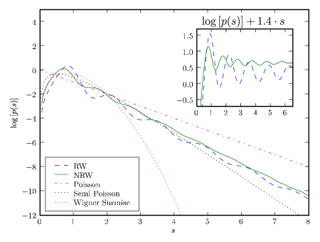
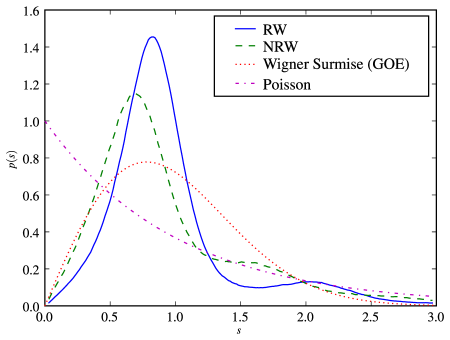
When considering the statistics of a sequence of points, the nearest neighbour spacing distribution (where the spacing is measured in units of the mean spacing) is perhaps the most natural, and easy to evaluate experimentally. In figure 1 we show the nearest neighbour distributions for two point processes. The first is the intersections of the nodal lines of the random wave (RW) field (2) with the reference curve. The second process (NRW) is the zeros of the normal derivative of the random waves on the curve. The distributions were generated by numerical simulations, and compared with the corresponding statistics of the random (Poisson) ensemble and the Wigner surmise (corresponding to the GOE ensemble) [20].
Refer to caption
Figure 1: Density of the nearest neighbour level spacing.

At short ranges, both ensembles display linear level repulsion similar to the GOE distribution, but with different slopes. The most conspicuous differences appear at large spacings, and to get a clearer impression, we show in figure 2, the same data in semi-log plot. We observe two important differences.

  1. 1.

    On average, both distributions decay exponentially with approximately the same rate p(s)exp(1.4s)similar-to𝑝𝑠1.4𝑠p(s)\sim\exp(-1.4s). This decay is faster than the exp(s)𝑠\exp(-s) Poisson decay, but slower the “Semi Poisson” [21] distribution, which decays like exp(2s)2𝑠\exp(-2s).

  2. 2.

    The overall exponential decays are decorated by persistent oscillations, which are clearly seen in the inset of figure 2. The oscillations have slowly decaying amplitudes and their frequencies are 1.4πsimilar-toabsent1.4𝜋\sim 1.4\pi for RW and 2πsimilar-toabsent2𝜋\sim 2\pi for NRW.

Refer to caption
Figure 2: Nearest neighbour level spacing (log density). Inset shows persistent oscillations relative to the mean decaying curve.

The results above demonstrate that the nodal intersection statistics are significantly different than those of other, well known, point processes. The purpose of this work is to investigate the reasons for the occurrence of these differences. However, the nearest neighbour statistic is not easily amenable to analytic derivation. Rather, we use the two point correlation function, which is readily accessible, as will be shown in this paper. For the asymptotic s1much-less-than𝑠1s\ll 1 limit, this statistic coincides with the nearest neighbour density. Furthermore, other statistics with well defined physical meaning, such as the power spectrum and number variance can be expressed in terms of the correlation. We will now give some definitions, and follow with an overview of a derivation for the two point correlation of nodal intersections with a general reference curve.

2.2 Two point correlations

A random field ψ(r)𝜓r\psi(\bi{r}) is Gaussian if for any vector uu\bi{u} whose elements u1,u2,,unsubscript𝑢1subscript𝑢2subscript𝑢𝑛u_{1},u_{2},\ldots,u_{n} are field amplitudes ui=ψ(ri)subscript𝑢𝑖𝜓subscriptriu_{i}=\psi(\bi{r}_{i}) or partial derivatives of the field at some points r1,,rnsubscriptr1bold-…subscriptrn\bi{r}_{1},\ldots,\bi{r}_{n}, the probability distribution of uu\bi{u} is multivariate normal. The probability density of a multivariate normal random vector uu\bi{u}, with mean value u0subscriptu0\bi{u}_{0} is given by

p(u)=1(2𝝅)n/2𝐝𝐞𝐭C𝐞𝐱𝐩[12(uu0)TC1(uu0)],𝑝u1superscript2𝝅n2C12superscriptusubscriptu0TsuperscriptC1usubscriptu0p(\bi{u})=\frac{1}{{(2\pi)}^{n/2}\sqrt{\det C}}\exp\!\!\left[-\frac{1}{2}{(\bi{u}-\bi{u}_{0})}^{T}C^{-1}(\bi{u}-\bi{u}_{0})\right], (8)

where C𝐶C is the covariance matrix Ci,j=Cov(ui,uj)subscript𝐶𝑖𝑗Covsubscript𝑢𝑖subscript𝑢𝑗C_{i,j}=\mathop{\mathrm{Cov}}\nolimits(u_{i},u_{j}). For the random wave ensemble (2), Gaussianity follows from the n𝑛n dimensional central limit theorem.

Assuming smoothness of the field, means and covariances of the field’s derivatives can be calculated by deriving the appropriate amplitude statistics. Combining that with the fact that all the elements of u0subscriptu0\bi{u}_{0} and C𝐶C are single point means and two point covariances, it follows that all statistical properties of a Gaussian field ψ(r)𝜓r\psi(\bi{r}) are completely determined by its mean value ψ(r)delimited-⟨⟩𝜓r\langle\psi(\bi{r})\rangle (which will be zero for the relevant cases investigated) and the two point covariance function G(r,r)𝐂𝐨𝐯(𝝍(r),𝝍(r))𝐺rsuperscriptrbold-′𝐂𝐨𝐯𝝍r𝝍superscriptrbold-′G(\bi{r},\bi{r^{\prime}})\equiv\mathop{\mathrm{Cov}}\nolimits(\psi(\bi{r}),\psi(\bi{r}^{\prime})). As a consequence, we should be able to extract the distribution of the zeros from this function, and, in particular, the correlation function of the nodal intersections can be derived from the correlation function of the 1 dimensional restriction f(t)ψ(r(t))𝑓𝑡𝜓rtf(t)\equiv\psi(\bi{r}(t)) of the investigated field to the given reference curve Γ:[0,L]2r(t):Γ0𝐿superscript2rt\Gamma:[0,L]\rightarrow\mathbb{R}^{2}\equiv\bi{r}(t) (t𝑡t is the natural curve parameter).

The density and correlations of nodal intersections (NI) can be calculated directly once f(t)𝑓𝑡f(t) and its properties are known, in particular we shall use the two point correlations of the restricted field f𝑓f and its derivative along the curve f˙(t)f/t˙𝑓𝑡differential-d𝑓differential-d𝑡\dot{f}(t)\equiv\rmd f/\rmd t:

C0(t,t)Cov(f(t),f(t))subscript𝐶0𝑡superscript𝑡Cov𝑓𝑡𝑓superscript𝑡\displaystyle C_{0}(t,t^{\prime})\equiv\mathop{\mathrm{Cov}}\nolimits\!\!\left(f(t),f(t^{\prime})\right)
C1(t,t)Cov(f(t),f˙(t)),C~1(t,t)Cov(f˙(t),f(t))formulae-sequencesubscript𝐶1𝑡superscript𝑡Cov𝑓𝑡˙𝑓superscript𝑡subscript~𝐶1𝑡superscript𝑡Cov˙𝑓𝑡𝑓superscript𝑡\displaystyle C_{1}(t,t^{\prime})\equiv\mathop{\mathrm{Cov}}\nolimits\!\!\left(f(t),\dot{f}(t^{\prime})\right),\quad\tilde{C}_{1}(t,t^{\prime})\equiv\mathop{\mathrm{Cov}}\nolimits\!\!\left(\dot{f}(t),f(t^{\prime})\right) (9)
C2(t,t)Cov(f˙(t),f˙(t))subscript𝐶2𝑡superscript𝑡Cov˙𝑓𝑡˙𝑓superscript𝑡\displaystyle C_{2}(t,t^{\prime})\equiv\mathop{\mathrm{Cov}}\nolimits\!\!\left(\dot{f}(t),\dot{f}(t^{\prime})\right)

We will also use lowercase c𝑐c to denote the single point limit of these, i.e. c0(t)C0(t,t)=Var(f(t))subscript𝑐0𝑡subscript𝐶0𝑡𝑡Var𝑓𝑡c_{0}(t)\equiv C_{0}(t,t)=\mathop{\mathrm{Var}}\nolimits\!\left(f(t)\right) etc.

2.3 Restricting the field to a curve

Before we write down expressions for C0subscript𝐶0C_{0}, C1subscript𝐶1C_{1} and C2subscript𝐶2C_{2}, let us take note of special properties of these functions, which follow from the symmetry of our field. The fields considered are translationally invariant. This implies that the mean and the variance of the field are constant over the domain. It allows us to apply a constant linear transformation ψ=Aψ~+B𝜓𝐴~𝜓𝐵\psi=A\tilde{\psi}+B, normalizing the field so that ψ(r)=0delimited-⟨⟩𝜓r0\langle\psi(\bi{r})\rangle=0 and c0=ψ2(r)=1subscript𝑐0delimited-⟨⟩superscript𝜓2r1c_{0}=\langle\psi^{2}\left(\bi{r}\right)\rangle=1 for all rr\bi{r} (this is true for equations (2) and (3), however we will keep c0subscript𝑐0c_{0} in our expressions below, to make explicit the effect of the multiplicative scaling).

Furthermore, assuming smoothness of ψ𝜓\psi, it follows that

2ψ(r)𝝍(r)=𝝍2(r)=0.2delimited-⟨⟩𝜓rbold-▽𝝍rbold-▽delimited-⟨⟩superscript𝝍2r02\langle\psi(\bi{r})\triangledown\psi(\bi{r})\rangle=\triangledown\langle\psi^{2}\left(\bi{r}\right)\rangle=0. (10)

In general, the restricted fields are not translationally invariant. Therefore the computation of their correlations requires special attention, and will involve the geometric properties of the reference curve, such as its curvature. However, in the limit tt𝑡superscript𝑡t\rightarrow t^{\prime}, one can still project (10) onto the curve, and conclude that C~1(t,t)C1(t,t)subscript~𝐶1𝑡superscript𝑡subscript𝐶1𝑡superscript𝑡\tilde{C}_{1}(t,t^{\prime})\rightarrow-C_{1}(t,t^{\prime}), and in particular c1=0subscript𝑐10c_{1}=0.

The fields we consider here are also isotropic111An example of a random field which is not isotropic, is the non-monochromatic random wave models used in [6], which have a finite average wavenumber vector (carrier wave), so the correlation function has the form ψ(r)𝝍(r)=G(|rr|)delimited-⟨⟩𝜓r𝝍superscriptrbold-′Grsuperscriptrbold-′\langle\psi(\bi{r})\psi(\bi{r}^{\prime})\rangle=G(|\bi{r}-\bi{r}^{\prime}|). To make use of this property, we change the coordinates

u=r+r,d=rr,formulae-sequenceursuperscriptrbold-′drsuperscriptrbold-′\bi{u}=\bi{r}+\bi{r}^{\prime},\quad\bi{d}=\bi{r}-\bi{r}^{\prime},

so that derivatives with respect to uu\bi{u} vanish. Derivatives with respect to dd\bi{d} can be expressed in terms of the single parameter function G(d)𝐺𝑑G(d) (where d=|d|𝑑dd=|\bi{d}|).

This results in the following expressions for the correlation functions (2.2)

C0=G(d)subscript𝐶0𝐺𝑑\displaystyle C_{0}=G(d)
C1=r˙d^G(d),C~1=r˙d^G(d)formulae-sequencesubscript𝐶1˙superscriptrbold-′^dsuperscript𝐺𝑑subscript~𝐶1˙r^dsuperscript𝐺𝑑\displaystyle C_{1}=-\dot{\bi{r}^{\prime}}\cdot\hat{\bi{d}}\,G^{\prime}(d),\quad\tilde{C}_{1}=\dot{\bi{r}}\cdot\hat{\bi{d}}\,G^{\prime}(d) (11)
C2=i,jr˙i[(G′′Gd)didjd2+Gdδi,j]r˙jsubscript𝐶2subscript𝑖𝑗subscript˙𝑟𝑖delimited-[]superscript𝐺′′superscript𝐺𝑑subscript𝑑𝑖subscript𝑑𝑗superscript𝑑2superscript𝐺𝑑subscript𝛿𝑖𝑗subscriptsuperscript˙𝑟𝑗\displaystyle C_{2}=-\sum_{i,j}\dot{r}_{i}\left[\left(G^{\prime\prime}-\frac{G^{\prime}}{d}\right)\frac{d_{i}d_{j}}{d^{2}}+\frac{G^{\prime}}{d}\delta_{i,j}\right]{\dot{r}^{\prime}}_{j}

where rr(t)superscriptrbold-′rsuperscripttbold-′\bi{r}^{\prime}\equiv\bi{r}(t^{\prime}), and d^d/d^ddd\hat{\bi{d}}\equiv\bi{d}/d.

2.4 The nodal intersections statistics

The density of zeros of f𝑓f takes the form

ρ(t)=iδ(tti)=δ(f(t))|f˙(t)|,where f(ti)=0.formulae-sequence𝜌𝑡subscript𝑖𝛿𝑡subscript𝑡𝑖𝛿𝑓𝑡˙𝑓𝑡where 𝑓subscript𝑡𝑖0\rho(t)=\sum_{i}\delta(t-t_{i})=\delta\!\left(f(t)\right)|\dot{f}(t)|,\quad\textrm{where }f(t_{i})=0. (12)

Following M. Kac [22], we use the Fourier representation:

ρ(t)=12π2ξηη2ξf(t)(1ηf˙(t)).delimited-⟨⟩𝜌𝑡12superscript𝜋2superscriptsubscriptdifferential-d𝜉differential-d𝜂superscript𝜂2delimited-⟨⟩superscript𝜉𝑓𝑡1superscript𝜂˙𝑓𝑡\langle\rho(t)\rangle=\frac{1}{2\pi^{2}}\int\!\!\!\int_{-\infty}^{\infty}\frac{\rmd\xi\,\rmd\eta}{\eta^{2}}\left\langle\rme^{\rmi\xi f(t)}(1-\rme^{\rmi\eta\dot{f}(t)})\right\rangle.

This integral can be solved using elementary properties of multinormal variables (8). For any multinormal variable xx\bi{x} with zero mean, and real vector kk\bi{k}, the following identity holds:

kx=exp(12i,jkiCi,jkj)where Ci,j=Cov(xi,xj)formulae-sequencedelimited-⟨⟩superscriptbold-⋅kx12subscript𝑖𝑗subscript𝑘𝑖subscript𝐶𝑖𝑗subscript𝑘𝑗where subscript𝐶𝑖𝑗Covsubscript𝑥𝑖subscript𝑥𝑗\langle\rme^{\rmi\bi{k}\cdot\bi{x}}\rangle=\exp\left(-\frac{1}{2}\sum_{i,j}k_{i}C_{i,j}k_{j}\right)\quad\textrm{where }C_{i,j}=\mathop{\mathrm{Cov}}\nolimits(x_{i},x_{j}) (13)

Using the Gaussianity of the field f𝑓f, this identity can be applied to the mean density. The resulting integral separates into simple Gaussian integrals, and we get the following result for the density:

ρ=1πc2c0delimited-⟨⟩𝜌1𝜋subscript𝑐2subscript𝑐0\left\langle\rho\right\rangle=\frac{1}{\pi}\sqrt{\frac{c_{2}}{c_{0}}} (14)

We now move on to two point statistics. When dealing with “point processes” (such as the zeros of f𝑓f), whose amplitude is a sum of delta functions, ρρdelimited-⟨⟩𝜌superscript𝜌\langle\rho\rho^{\prime}\rangle normally contains a delta function at t=t𝑡superscript𝑡t=t^{\prime}, corresponding to the strong autocorrelation. It is customary to subtract this term, to regularize the correlation function at t=t𝑡superscript𝑡t=t^{\prime}. Thus, the two point correlation function is defined (e.g. in [20]) as

R(t,t)𝑅𝑡superscript𝑡\displaystyle R(t,t^{\prime}) =ijδ(tti)δ(ttj)absentdelimited-⟨⟩subscript𝑖𝑗𝛿𝑡subscript𝑡𝑖𝛿superscript𝑡subscript𝑡𝑗\displaystyle=\left\langle\sum_{i\neq j}\delta(t-t_{i})\delta(t^{\prime}-t_{j})\right\rangle
=ρ(t)ρ(t)δ(tt)ρ(t).absentdelimited-⟨⟩𝜌𝑡𝜌superscript𝑡𝛿𝑡superscript𝑡delimited-⟨⟩𝜌𝑡\displaystyle=\langle\rho(t)\rho(t^{\prime})\rangle-\delta(t-t^{\prime})\langle\rho(t)\rangle.

Using the same approach as above, we write:

ρρ=14π4ξηξηη2η2ξf(1ηf˙)ξf(1ηf˙)delimited-⟨⟩𝜌superscript𝜌delimited-⟨⟩14superscript𝜋4differential-d𝜉differential-d𝜂differential-dsuperscript𝜉differential-dsuperscript𝜂superscript𝜂2superscript𝜂2superscript𝜉𝑓1superscript𝜂˙𝑓superscriptsuperscript𝜉superscript𝑓1superscriptsuperscript𝜂superscript˙𝑓\langle\rho\rho^{\prime}\rangle=\left\langle\frac{1}{4\pi^{4}}\int\frac{\rmd\xi\,\rmd\eta\,\rmd\xi^{\prime}\,\rmd\eta^{\prime}}{\eta^{2}\eta^{\prime 2}}\rme^{\rmi\xi f}(1-\rme^{\rmi\eta\dot{f}})\rme^{\rmi\xi^{\prime}f^{\prime}}(1-\rme^{\rmi\eta^{\prime}\dot{f}^{\prime}})\right\rangle (15)

To make use of (13), we write down the covariance matrix of the four variables (f,f,f˙,f˙)𝑓superscript𝑓˙𝑓superscript˙𝑓(f,f^{\prime},\dot{f},\dot{f}^{\prime}) appearing in this expression (see definitions in (2.2)):

M=(c0C00C1C0c0C~100C~1c2C2C10C2c2)(ACCTB)𝑀subscript𝑐0subscript𝐶00subscript𝐶1subscript𝐶0subscript𝑐0subscript~𝐶100subscript~𝐶1subscript𝑐2subscript𝐶2subscript𝐶10subscript𝐶2subscript𝑐2𝐴𝐶superscript𝐶𝑇𝐵M=\left(\begin{array}[]{cccc}c_{0}&C_{0}&0&C_{1}\\ C_{0}&c_{0}&\tilde{C}_{1}&0\\ 0&\tilde{C}_{1}&c_{2}&C_{2}\\ C_{1}&0&C_{2}&c_{2}\end{array}\right)\equiv\left(\begin{array}[]{cc}A&C\\ C^{T}&B\end{array}\right) (16)

(A𝐴A,B𝐵B,C𝐶C stand for the 2×2222\times 2 submatrices).

Applying (13) to (15) we get more complicated integrals, which are nevertheless solvable (derivation in A). The resulting expression for R(t,t)𝑅𝑡superscript𝑡R(t,t^{\prime}) is

R(t,t)=1π2a|A|3/2(1c^2+c^arcsin(c^)),𝑅𝑡superscript𝑡1superscript𝜋2𝑎superscript𝐴321superscript^𝑐2^𝑐^𝑐R(t,t^{\prime})=\frac{1}{\pi^{2}}\frac{a}{|A|^{3/2}}\left(\sqrt{1-\hat{c}^{2}}+\hat{c}\arcsin(\hat{c})\right),

where a=c2|A|c0|C|𝑎subscript𝑐2𝐴subscript𝑐0𝐶a=c_{2}|A|-c_{0}|C|, c^=(C2|A|C0|C|)/a^𝑐subscript𝐶2𝐴subscript𝐶0𝐶𝑎\hat{c}=(C_{2}|A|-C_{0}|C|)/a, |A|=c02C02𝐴superscriptsubscript𝑐02superscriptsubscript𝐶02|A|={c_{0}}^{2}-{C_{0}}^{2} and |C|=C1C~1𝐶subscript𝐶1subscript~𝐶1|C|=-C_{1}\tilde{C}_{1} (here |A|𝐴|A| and |C|𝐶|C| stand for determinants—not absolute value).

From this, the normalized correlation coefficient R/ρ21𝑅superscriptdelimited-⟨⟩𝜌21\mathcal{R}\equiv R/{\langle\rho\rangle}^{2}-1, from which we will derive the other two point statistics, follows immediately:

(t,t)=c0c2a|A|3/2(1c^2+c^arcsin(c^))1𝑡superscript𝑡subscript𝑐0subscript𝑐2𝑎superscript𝐴321superscript^𝑐2^𝑐^𝑐1\mathcal{R}(t,t^{\prime})=\frac{c_{0}}{c_{2}}\frac{a}{|A|^{3/2}}\left(\sqrt{1-\hat{c}^{2}}+\hat{c}\arcsin(\hat{c})\right)-1 (17)

3 Simple curves in monochromatic random fields

The monochromatic Gaussian field (2) is often used as a statistical model for eigenfunctions of chaotic billiards. In this context, the “semiclassical” regime (large k𝑘k) has special significance. In terms of our statistical system, this means that we would be particularly interested in the kκmuch-greater-than𝑘𝜅k\gg\kappa limit (where κ𝜅\kappa is the curvature of the reference curve). In this regime, the first approximation for the curve is a straight line, and the second one is a circular arc. These two cases are also important for their simplicity—in both cases, the domain distance d𝑑d between two points on the curve depends only on the curve distance |tt|𝑡superscript𝑡|t-t^{\prime}|, so (2.3) assumes a simpler form.

For the straight line, r˙=d^˙r^d\dot{\bi{r}}=\hat{\bi{d}} is constant and d=|tt|𝑑𝑡superscript𝑡d=|t-t^{\prime}|. We get:

C0=G(d),C1=G(d),C2=G′′(d)formulae-sequencesubscript𝐶0𝐺𝑑formulae-sequencesubscript𝐶1superscript𝐺𝑑subscript𝐶2superscript𝐺′′𝑑C_{0}=G(d),\quad C_{1}=-G^{\prime}(d),\quad C_{2}=-G^{\prime\prime}(d) (18a)

For a circle of radius r𝑟r, define α(tt)/(2r)𝛼𝑡superscript𝑡2𝑟\alpha\equiv(t-t^{\prime})/(2r), so d=2rsinα𝑑2𝑟𝛼d=2r\sin\alpha, and by simple geometrical identities, we get:

C0=G(d),C1=cosαG(d),formulae-sequencesubscript𝐶0𝐺𝑑subscript𝐶1𝛼superscript𝐺𝑑\displaystyle C_{0}=G(d),\quad C_{1}=-\cos\alpha G^{\prime}(d),
C2=sin2αG(d)dcos2αG′′(d)subscript𝐶2superscript2𝛼superscript𝐺𝑑𝑑superscript2𝛼superscript𝐺′′𝑑\displaystyle C_{2}=\sin^{2}\alpha\frac{G^{\prime}(d)}{d}-\cos^{2}\alpha G^{\prime\prime}(d) (18b)

3.1 Normalized correlation for the line and the circle

Substituting (4) in (18a) and (18b), we get the amplitude correlations. The results for the circle are (the straight line is given by their α0𝛼0\alpha\rightarrow 0 limit):

C0=J0(kd)subscript𝐶0subscript𝐽0𝑘𝑑\displaystyle C_{0}=J_{0}(kd)
C1=kcos(α)J1(kd)subscript𝐶1𝑘𝛼subscript𝐽1𝑘𝑑\displaystyle C_{1}=k\cos(\alpha)J_{1}(kd) (18s)
C2=k2(J0(kd)cos2(α)J1(kd)kd)subscript𝐶2superscript𝑘2subscript𝐽0𝑘𝑑superscript2𝛼subscript𝐽1𝑘𝑑𝑘𝑑\displaystyle C_{2}=k^{2}\left(J_{0}(kd)\cos^{2}(\alpha)-\frac{J_{1}(kd)}{kd}\right)

For the density, we substitute c2=C2(0)=12k2subscript𝑐2subscript𝐶2012superscript𝑘2c_{2}=C_{2}(0)=\frac{1}{2}k^{2} in (14) getting ρ=k/(2π)delimited-⟨⟩𝜌𝑘2𝜋\langle\rho\rangle={k}/(\sqrt{2}\pi). We use this to select a curve parameter which measures length in units of average spacing (so we can expect meaningful results at the ρdelimited-⟨⟩𝜌\langle\rho\rangle\rightarrow\infty limit):

s(tt)ρ=(tt)k/(2π).𝑠superscript𝑡𝑡delimited-⟨⟩𝜌𝑡superscript𝑡𝑘2𝜋s\equiv(t^{\prime}-t)\langle\rho\rangle={(t-t^{\prime})k}/(\sqrt{2}\pi).

In the new units, α=s2π/(2kr)𝛼𝑠2𝜋2𝑘𝑟\alpha=s\sqrt{2}\pi/(2kr) and the argument of the Bessel functions is

θkd=2krsin(2πs2kr)\mathsm@sh\mathsm@shkr2πs𝜃𝑘𝑑2𝑘𝑟2𝜋𝑠2𝑘𝑟subscriptlimit-from\mathsm@shlimit-from\mathsm@sh𝑘𝑟2𝜋𝑠\theta\equiv kd=2kr\sin\!\!\left(\frac{\sqrt{2}\pi s}{2kr}\right)\mathrel{\mathop{\hbox to112.77734pt{\hbox{$\displaystyle\mathrel{\mathchoice{\mathsm@sh\displaystyle{\mathchar 45\relax}}{\mathsm@sh\textstyle{\mathchar 45\relax}}{\mathsm@sh\scriptstyle{\mathchar 45\relax}}{\mathsm@sh\scriptscriptstyle{\mathchar 45\relax}}}\mkern-7.0mu\cleaders\hbox{$\displaystyle\mkern-2.0mu\mathrel{\mathchoice{\mathsm@sh\displaystyle{\mathchar 45\relax}}{\mathsm@sh\textstyle{\mathchar 45\relax}}{\mathsm@sh\scriptstyle{\mathchar 45\relax}}{\mathsm@sh\scriptscriptstyle{\mathchar 45\relax}}}\mkern-2.0mu$}\hfill\mkern-7.0mu\rightarrow$}}}\limits_{kr\rightarrow\infty\mkern 3.0mu}}\sqrt{2}\pi s

For the NI normalized correlation, we substitute (3.1) in (17), getting:

c^=[J0(θ)cos2αJ1(θ)/θ][1J0(θ)2]J0(θ)J12(θ)cos2α[1J02(θ)]/2J12(θ)cos2α^𝑐delimited-[]subscript𝐽0𝜃superscript2𝛼subscript𝐽1𝜃𝜃delimited-[]1subscript𝐽0superscript𝜃2subscript𝐽0𝜃superscriptsubscript𝐽12𝜃superscript2𝛼delimited-[]1superscriptsubscript𝐽02𝜃2superscriptsubscript𝐽12𝜃superscript2𝛼\displaystyle\hat{c}=\frac{\left[J_{0}(\theta)\cos^{2}\alpha-J_{1}(\theta)/\theta\right]\left[1-{J_{0}(\theta)}^{2}\right]-J_{0}(\theta){J_{1}}^{2}(\theta)\cos^{2}\alpha}{\left[1-{J_{0}}^{2}(\theta)\right]/2-{J_{1}}^{2}(\theta)\cos^{2}\alpha}
=1J02(θ)2J12(θ)cos2α[1J02(θ)]3/2(1c^2+c^arcsinc^)11superscriptsubscript𝐽02𝜃2superscriptsubscript𝐽12𝜃superscript2𝛼superscriptdelimited-[]1superscriptsubscript𝐽02𝜃321superscript^𝑐2^𝑐^𝑐1\displaystyle\mathcal{R}=\frac{1-{J_{0}}^{2}(\theta)-2{J_{1}}^{2}(\theta)\cos^{2}\alpha}{{\left[1-{J_{0}}^{2}(\theta)\right]}^{3/2}}\left(\sqrt{1-{\hat{c}}^{2}}+\hat{c}\arcsin\hat{c}\right)-1 (18t)

To get the universal distribution (k𝑘k independent, high density limit), we take k𝑘k\rightarrow\infty keeping s𝑠s constant.

c^=[J0(θ)J1(θ)/θ][1J0(θ)2]J0(θ)J12(θ)[1J02(θ)]/2J12(θ)^𝑐delimited-[]subscript𝐽0𝜃subscript𝐽1𝜃𝜃delimited-[]1subscript𝐽0superscript𝜃2subscript𝐽0𝜃superscriptsubscript𝐽12𝜃delimited-[]1superscriptsubscript𝐽02𝜃2superscriptsubscript𝐽12𝜃\displaystyle\hat{c}=\frac{\left[J_{0}(\theta)-J_{1}(\theta)/\theta\right]\left[1-{J_{0}(\theta)}^{2}\right]-J_{0}(\theta){J_{1}}^{2}(\theta)}{\left[1-{J_{0}}^{2}(\theta)\right]/2-{J_{1}}^{2}(\theta)}
=1J02(θ)2J12(θ)[1J02(θ)]3/2(1c^2+c^arcsinc^)11superscriptsubscript𝐽02𝜃2superscriptsubscript𝐽12𝜃superscriptdelimited-[]1superscriptsubscript𝐽02𝜃321superscript^𝑐2^𝑐^𝑐1\displaystyle\mathcal{R}=\frac{1-{J_{0}}^{2}(\theta)-2{J_{1}}^{2}(\theta)}{{\left[1-{J_{0}}^{2}(\theta)\right]}^{3/2}}\left(\sqrt{1-{\hat{c}}^{2}}+\hat{c}\arcsin\hat{c}\right)-1 (18u)

Note that in the case of the straight line (κ1/r0𝜅1𝑟0\kappa\equiv 1/r\rightarrow 0), we have θ=2πs𝜃2𝜋𝑠\theta=\sqrt{2}\pi s and α=0𝛼0\alpha=0 exactly, so there is no k𝑘k dependence, and the universal function (18u) is exact for any k𝑘k (this is expected, because with no boundary and no curvature, the system has no natural scale).

To further study the universal correlation function (18u), we derive its asymptotic expansion. The first few terms in the expansion of (s)𝑠\mathcal{R}(s) near s=0𝑠0s=0 are:

1+π216s+37π42304s3+π412962s4.1superscript𝜋216𝑠37superscript𝜋42304superscript𝑠3superscript𝜋412962superscript𝑠4-1+\frac{\pi^{2}}{16}s+\frac{37\pi^{4}}{2304}s^{3}+\frac{\pi^{4}}{1296\sqrt{2}}s^{4}. (18v)

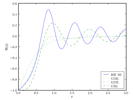
This rises linearly from 11-1, with a smaller slope than the GOE ensemble (other RMT ensembles are not linear at this limit), however, as is shown in figure 3, it rises quicker to positive values, resulting in a smaller range of high repulsion.
Refer to caption
Figure 3: Normalized Correlation: NI of RW vs RMT level spacings.

For large values of s𝑠s, we find decaying terms, oscillating in frequencies which are multiples of the dominant frequency ω2π2𝜔2𝜋2\omega\equiv 2\pi\sqrt{2}. The asymptotic expansion has the form:

(s)Ren=131(πωs)nm=0nqn,m(π)m(ωsπ/2)+O(s4)similar-to𝑠Resuperscriptsubscript𝑛131superscript𝜋𝜔𝑠𝑛superscriptsubscript𝑚0𝑛subscript𝑞𝑛𝑚𝜋superscript𝑚𝜔𝑠𝜋2Big-Osuperscript𝑠4\mathcal{R}(s)\sim\mathop{\mathrm{Re}}\nolimits\sum_{n=1}^{3}\frac{1}{{(\pi\omega s)}^{n}}\sum_{m=0}^{n}q_{n,m}(\rmi\pi)\rme^{\rmi m(\omega s-\pi/2)}+\Or(s^{-4}) (18w)

where qn,m(x)subscript𝑞𝑛𝑚𝑥q_{n,m}(x) are the following polynomials:

q1,0=1,q1,1=9formulae-sequencesubscript𝑞101subscript𝑞119\displaystyle q_{1,0}=1,\quad q_{1,1}=9
q2,0=254,q2,1=493+392x,q2,2=12112formulae-sequencesubscript𝑞20254formulae-sequencesubscript𝑞21493392𝑥subscript𝑞2212112\displaystyle q_{2,0}=\frac{25}{4},\quad q_{2,1}=\frac{49}{3}+\frac{39}{2}x,\quad q_{2,2}=\frac{121}{12}
q3,0=1694+172x2,q3,1=136924+5116x+2058x2,formulae-sequencesubscript𝑞301694172superscript𝑥2subscript𝑞311369245116𝑥2058superscript𝑥2\displaystyle q_{3,0}=\frac{169}{4}+\frac{17}{2}x^{2},\quad q_{3,1}=\frac{1369}{24}+\frac{511}{6}x+\frac{205}{8}x^{2},
q3,2=168160+5512x,q3,3=52940formulae-sequencesubscript𝑞321681605512𝑥subscript𝑞3352940\displaystyle\qquad q_{3,2}=\frac{1681}{60}+\frac{55}{12}x,\quad q_{3,3}=\frac{529}{40}

Writing the leading terms explicitly, we have

1πωs(1+9sin(ωs))similar-to1𝜋𝜔𝑠19𝜔𝑠\mathcal{R}\sim\frac{1}{\pi\omega s}\left(1+9\sin(\omega s)\right) (18x)

This s1superscript𝑠1s^{-1} decay is slower than the decay of random matrix ensembles (s2superscript𝑠2s^{-2} for GOE and GUE, and s1×[oscillatingpart]superscript𝑠1delimited-[]oscillatingparts^{-1}\times[\mathrm{oscillating\ part}] for GSE). The slow decay has a considerable effect on all statistics that probe large distances, as will be shown in section 3.2.

When we look at intersections on a full circle, s𝑠s goes over all values, from kr/2𝑘𝑟2-kr/\sqrt{2} to kr/2𝑘𝑟2kr/\sqrt{2}. This range contains values large enough to make (18u) unsuitable for approximating the correlations. The leading terms in the asymptotic expansion of (18t) (the equivalent of (18x)) are found to be:

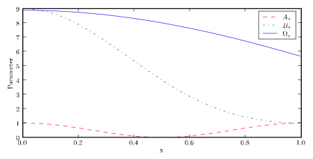
(s)=1πΩss(As+Bssin(Ωss))+O(s2)𝑠1𝜋subscriptΩ𝑠𝑠subscript𝐴𝑠subscript𝐵𝑠subscriptΩ𝑠𝑠Big-Osuperscript𝑠2\mathcal{R}(s)=\frac{1}{\pi\Omega_{s}s}\left(A_{s}+B_{s}\sin(\Omega_{s}s)\right)+\Or(s^{-2}) (18y)

where

As=cos2(2πs2kr),Bs=[2+cos(2πs2kr)]2,formulae-sequencesubscript𝐴𝑠superscript22𝜋𝑠2𝑘𝑟subscript𝐵𝑠superscriptdelimited-[]22𝜋𝑠2𝑘𝑟2\displaystyle A_{s}=\cos^{2}\!\!\left(\frac{2\pi s}{\sqrt{2}kr}\right),B_{s}={\left[2+\cos\!\!\left(\frac{2\pi s}{\sqrt{2}kr}\right)\right]}^{2},
Ωs=sinc(s2kr)ωsubscriptΩ𝑠sinc𝑠2𝑘𝑟𝜔\displaystyle\Omega_{s}=\mathop{\mathrm{sinc}}\nolimits\!\!\left(\frac{s}{\sqrt{2}kr}\right)\cdot\omega

(with normalized sinc(x)sin(πx)/(πx)sinc𝑥𝜋𝑥𝜋𝑥\mathop{\mathrm{sinc}}\nolimits(x)\equiv\sin(\pi x)/(\pi x)), are slowly varying functions, starting from A0=1subscript𝐴01A_{0}=1,B0=9subscript𝐵09B_{0}=9 and Ω0=ωsubscriptΩ0𝜔\Omega_{0}=\omega (as expected from (18x), which holds for skrmuch-less-than𝑠𝑘𝑟s\ll kr), and ending in A±S=1subscript𝐴plus-or-minus𝑆1A_{\pm S}=1,B±S=1subscript𝐵plus-or-minus𝑆1B_{\pm S}=1 and Ω±S=42subscriptΩplus-or-minus𝑆42\Omega_{\pm S}=4\sqrt{2} for S=kr/2𝑆𝑘𝑟2S=kr/\sqrt{2}. The functions Assubscript𝐴𝑠A_{s}, Bssubscript𝐵𝑠B_{s} and ΩssubscriptΩ𝑠\Omega_{s} are illustrated in figure 4. As we increase k𝑘k, the rate of change becomes slower, but the normalized length of the curve increases, and the value of the coefficients for maximally separated points (|s|=kr/2𝑠𝑘𝑟2|s|=kr/\sqrt{2}) remains the same.

Refer to caption
Figure 4: Asymptotic coefficients and frequency for RW NI on half a circle as a function of x=2s/(kr)𝑥2𝑠𝑘𝑟x=\sqrt{2}s/(kr).

Before proceeding to compute other statistics, we would like to point out that the oscillations in p(s)𝑝𝑠p(s) (see section 2.1) have a frequency which is numerically consistent with half the dominant frequency ω2π2𝜔2𝜋2\omega\equiv 2\pi\sqrt{2}.

3.2 Number variance and power spectrum

The variance of the number of intersections in a finite segment of length L𝐿L is often used as a measure for the “rigidity” of the distribution (a completely rigid set of points will have zero variance). The power spectrum [17] measures periodicity in the distribution (which is also manifested by oscillations in the correlation function). These statistics are given by integral transforms of \mathcal{R} which are hard to solve directly. Instead, the asymptotic expansions of the correlation function can be used to expand them in series at regions of interest, as explained in C.

The variance for the number of intersections on a finite segment of length L𝐿L can be calculated from the normalized correlation by [20]:

Σ2(L)=L+20L(Ls)(s)ssuperscriptΣ2𝐿𝐿2superscriptsubscript0𝐿𝐿𝑠𝑠differential-d𝑠\Sigma^{2}(L)=L+2\int_{0}^{L}(L-s)\mathcal{R}(s)\rmd s (18z)

We can use (18v) and (18w) to find the asymptotic behaviour of this statistics. For small L𝐿L, we find

Σ2LL2+π248L3+37π423040L5+π4194402L6similar-tosuperscriptΣ2𝐿superscript𝐿2superscript𝜋248superscript𝐿337superscript𝜋423040superscript𝐿5superscript𝜋4194402superscript𝐿6\Sigma^{2}\sim L-L^{2}+\frac{\pi^{2}}{48}L^{3}+\frac{37\pi^{4}}{23040}L^{5}+\frac{\pi^{4}}{19440\sqrt{2}}L^{6}

The first two terms follow from the formal definition of Σ2superscriptΣ2\Sigma^{2}, and therefore coincide with the corresponding terms in the RMT ensembles. The third term corresponds to the probability of finding two intersections in the small interval [0,L]0𝐿[0,L]. It is of order L3superscript𝐿3L^{3}, as in GOE (again with a smaller factor).

For large L𝐿L, we find

Σ2similar-tosuperscriptΣ2absent\displaystyle\Sigma^{2}\sim 2q1,0(πω)(LlnLL)+L(1+2RW0)2subscript𝑞10𝜋𝜔𝐿𝐿𝐿𝐿12subscriptsuperscript0RW\displaystyle\frac{2q_{1,0}}{(\pi\omega)}(L\ln L-L)+L(1+2\mathcal{M}^{0}_{\mathrm{RW}}) (18aa)
2q2,0(πω)2(lnL+1)2RW12subscript𝑞20superscript𝜋𝜔2𝐿12subscriptsuperscript1RW\displaystyle-\frac{2q_{2,0}}{{(\pi\omega)}^{2}}(\ln L+1)-2\mathcal{M}^{1}_{\mathrm{RW}}
+1(πω)3LRe[q3,0(π)+2π2q1,1ωL]+O(L2)1superscript𝜋𝜔3𝐿Redelimited-[]subscript𝑞30𝜋2superscript𝜋2subscript𝑞11superscript𝜔𝐿Big-Osuperscript𝐿2\displaystyle+\frac{1}{{(\pi\omega)}^{3}L}\mathop{\mathrm{Re}}\nolimits\!\left[q_{3,0}(\rmi\pi)+2\rmi\pi^{2}q_{1,1}\rme^{\rmi\omega L}\right]+\Or(L^{-2})

where RW0subscriptsuperscript0RW\mathcal{M}^{0}_{\mathrm{RW}} and RW1subscriptsuperscript1RW\mathcal{M}^{1}_{\mathrm{RW}} are fixed constants, given by

RW0=subscriptsuperscript0RWabsent\displaystyle\mathcal{M}^{0}_{\mathrm{RW}}= 01(s)s+1[(s)1πωs]s0.336similar-tosuperscriptsubscript01𝑠differential-d𝑠superscriptsubscript1delimited-[]𝑠1𝜋𝜔𝑠differential-d𝑠0.336\displaystyle\int_{0}^{1}\mathcal{R}(s)\rmd s+\int_{1}^{\infty}\left[\mathcal{R}(s)-\frac{1}{\pi\omega s}\right]\rmd s\sim-0.336
RW1=subscriptsuperscript1RWabsent\displaystyle\mathcal{M}^{1}_{\mathrm{RW}}= 1πω(9cosωω1)+01s(s)s1𝜋𝜔9𝜔𝜔1superscriptsubscript01𝑠𝑠differential-d𝑠\displaystyle\frac{1}{\pi\omega}\left(9\frac{\cos\omega}{\omega}-1\right)+\int_{0}^{1}s\mathcal{R}(s)\rmd s
+1[s(s)1πω(1+9sinωs)254(πω)2s]ssuperscriptsubscript1delimited-[]𝑠𝑠1𝜋𝜔19𝜔𝑠254superscript𝜋𝜔2𝑠differential-d𝑠\displaystyle+\int_{1}^{\infty}\left[s\mathcal{R}(s)-\frac{1}{\pi\omega}(1+9\sin\omega s)-\frac{25}{4{(\pi\omega)}^{2}s}\right]\rmd s
0.0826similar-toabsent0.0826\displaystyle\sim-0.0826

Writing down the first terms of (18aa) explicitly, we have:

Σ2(L)similar-tosuperscriptΣ2𝐿absent\displaystyle\Sigma^{2}(L)\sim 2πωLlnL+(12πω+2RW0)L2𝜋𝜔𝐿𝐿12𝜋𝜔2subscriptsuperscript0RW𝐿\displaystyle\frac{2}{\pi\omega}L\ln L+\left(1-\frac{2}{\pi\omega}+2\mathcal{M}^{0}_{\mathrm{RW}}\right)L (18ab)
25(2πω)2lnL2(RW1+25(2πω)2)25superscript2𝜋𝜔2𝐿2subscriptsuperscript1RW25superscript2𝜋𝜔2\displaystyle-\frac{25}{{(2\pi\omega)}^{2}}\ln L-2\left(\mathcal{M}^{1}_{\mathrm{RW}}+\frac{25}{{(2\pi\omega)}^{2}}\right)

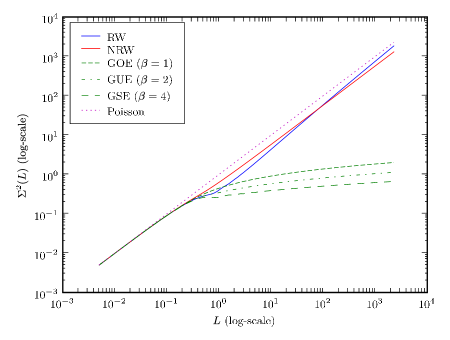
Note that this variance is asymptotically larger than that of the random (Poisson) distribution (where Σ2Lsimilar-tosuperscriptΣ2𝐿\Sigma^{2}\sim L). However, due to the numerical constants, the LlnL𝐿𝐿L\ln L term dominates only when L>exp(πω(RW0+1/2)1)36𝐿𝜋𝜔subscriptsuperscript0RW121similar-to36L>\exp(\pi\omega(\mathcal{M}^{0}_{\mathrm{RW}}+1/2)-1)\sim 36, and only at L32×103similar-to𝐿32superscript103L\sim 32\times 10^{3} does it become larger than the Poisson variance. At segments whose length is a few average spacings, the variance already becomes significantly larger than the “rigid” RMT ensembles. In figure 5, the variances of several distributions are compared.
Refer to caption
Figure 5: Number variance in segments of length L𝐿L. For large L𝐿L, the NRW curve is linear, hence parallel to the Poisson curve. The RW curve rises faster (the crossing point is at L32×103similar-to𝐿32superscript103L\sim 32\times 10^{3}, beyond the range of this plot).

It should be noted that in the case of independent site percolation (for grids with bounded, convex cells), a straight line passes only once through each cell. Hence the sign changes along the line form a Poisson process, with linear number variance. The fact that the asymptotic behaviour of the random wave model behaves differently is of interest, because the predictions of the percolation model [5] matched the numerical data for other parameters which characterize the behaviour of RW nodal lines in the high energy limit. Namely, the nodal count (number of nodal domains contained inside a given area) [4] and the SLE driving force [19].

The form factor (scaled power spectrum) for the intersections is the Fourier transform of the scaled correlation function (up to the subtraction of a δ(τ)𝛿𝜏\delta(\tau) term),

K(τ)𝐾𝜏\displaystyle K(\tau) =Γ2πτsρ(x)ρ(x+s)ρ2sδ(τ)absentsubscriptΓsuperscript2𝜋𝜏𝑠delimited-⟨⟩𝜌𝑥𝜌𝑥𝑠superscriptdelimited-⟨⟩𝜌2differential-d𝑠𝛿𝜏\displaystyle=\int_{\Gamma}\rme^{\rmi 2\pi\tau s}\frac{\langle\rho(x)\rho(x+s)\rangle}{{\langle\rho\rangle}^{2}}\rmd s-\delta(\tau) (18ac)
=1+Γ2πτs(s)s.absent1subscriptΓsuperscript2𝜋𝜏𝑠𝑠differential-d𝑠\displaystyle=1+\int_{\Gamma}\rme^{\rmi 2\pi\tau s}\mathcal{R}(s)\rmd s.

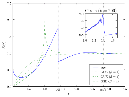
In figure 6 this is plotted and compared to the corresponding RMT values.

By (18x) it is clear that K𝐾K diverges for τ=0𝜏0\tau=0 (since 1/(πωs)1𝜋𝜔𝑠1/(\pi\omega s) is non integrable). Similarly, from the form of equation (18w), we expect singularities at integer multiples of 22\sqrt{2} (corresponding to the angular frequency ω=2π2𝜔2𝜋2\omega=2\pi\sqrt{2}). To quantify this, we use the asymptotic expansion of \mathcal{R} to expand K(τ)𝐾𝜏K(\tau) in small regions around the singular points τ=2n+δ𝜏2𝑛𝛿\tau=\sqrt{2}n+\delta for δ1much-less-than𝛿1\delta\ll 1.

For the divergence at 0 (τ1)much-less-than𝜏1(\tau\ll 1), we get

K(τ)1+2RW02[γ+ln(2π)]πω2πωlnτsimilar-to𝐾𝜏12subscriptsuperscript0RW2delimited-[]𝛾2𝜋𝜋𝜔2𝜋𝜔𝜏K(\tau)\sim 1+2\mathcal{M}^{0}_{\mathrm{RW}}-\frac{2[\gamma+\ln(2\pi)]}{\pi\omega}-\frac{2}{\pi\omega}\ln\tau

This is a logarithmic divergence. It drops down to 1 at τ08×106similar-tosubscript𝜏08superscript106\tau_{0}\sim 8\times 10^{-6} (which is too small to be observable in figure 6). The parameter K(0)=1+Γ(s)s𝐾01subscriptΓ𝑠differential-d𝑠K(0)=1+\int_{\Gamma}\mathcal{R}(s)\rmd s can be viewed as a measure of asymptotic spectral rigidity [23]. In our case, we see that we have “infinite softness”—the slow decay of the correlations outweighs the short distance repulsion.

One notable feature of figure 6, is the finite jump at τ=2𝜏2\tau=\sqrt{2}. Expanding for this region, we find

K(2+δ)similar-to𝐾2𝛿absent\displaystyle K\!\!\left(\sqrt{2}+\delta\right)\sim A+Bδ𝐴𝐵𝛿\displaystyle A+B\delta
92ωSign[δ]3916π|δ|+4912π3δln|δ|92𝜔Signdelimited-[]𝛿3916𝜋𝛿4912superscript𝜋3𝛿𝛿\displaystyle-\frac{9}{2\omega}\mathop{\mathrm{Sign}}\nolimits[\delta]-\frac{39}{16\pi}|\delta|+\frac{49}{12\pi^{3}}\delta\ln|\delta|

where A1.25similar-to𝐴1.25A\sim 1.25 and B1.53similar-to𝐵1.53B\sim 1.53 are numerical constants.

Refer to caption
Figure 6: Form factor for RW Nodal Intersections. The logarithmic divergence to ++\infty at τ=0𝜏0\tau=0 is too steep to be observable in this scale.

For the case where the reference line is a circle (inset of figure 6), we observe strong oscillations in the form factor for τ<2𝜏2\tau<\sqrt{2}. These oscillations are caused by the “drifting” of the frequency ΩssubscriptΩ𝑠\Omega_{s} in (18y). Their frequency increases for large values of k𝑘k, and we would expect them to cancel out when averaged over a wide enough window of frequencies.

4 The normal derivative of a Gaussian field

When dealing with solutions of boundary value problems (e.g. two dimensional quantum billiards), the boundary of the domain is a curve that plays a special role. It is therefore worthwhile to investigate its intersections with the nodal lines. For a Dirichlet boundary condition, the boundary is part of the nodal set, and the derivative of the eigenfunction in the tangent direction is zero. At the points where another nodal line intersects the boundary, the derivative in the direction of the other line will also vanish. Since nodal lines of solutions of the Helmholtz equation intersect at right angles, the intersections we wish to explore are also zeros of the normal derivative of the field with respect to the curve. This fact makes the normal derivative of other fields, such as the unbound random wave, natural candidates for comparison with the statistics of such intersections.

If fact, the normal derivative of a Gaussian random wave field is directly related to the “boundary modified” field mentioned in section 1. The boundary modified random waves [11], with correlation function approaching (5), might be realized by symmetrization of the unbound random wave field (2): ψBRW(x,y)ψ(x,y)ψ(x,y)subscript𝜓BRW𝑥𝑦𝜓𝑥𝑦𝜓𝑥𝑦\psi_{\mathrm{BRW}}(x,y)\equiv\psi(x,y)-\psi(x,-y) (where ψ=ψRW𝜓subscript𝜓RW\psi=\psi_{\mathrm{RW}} of (4)). In this case, the correlations on the boundary itself can be defined as the limit of correlations on a line parallel to the x𝑥x axis at y0+𝑦limit-from0y\rightarrow 0+. To get a meaningful limit we must introduce a y𝑦y-dependent scaling, to keep ψBRW2delimited-⟨⟩superscriptsubscript𝜓BRW2\langle{\psi_{\mathrm{BRW}}}^{2}\rangle constant as we approach y=0𝑦0y=0. Denoting ϕy(x)ψBRW(x,y)subscriptitalic-ϕ𝑦𝑥subscript𝜓BRW𝑥𝑦\phi_{y}(x)\equiv\psi_{\mathrm{BRW}}(x,y), the average square amplitude for a line at height y𝑦y is:

ϕy(x)2=(ψ(x,y)ψ(x,y))2=2(c0C0(2y))delimited-⟨⟩subscriptitalic-ϕ𝑦superscript𝑥2delimited-⟨⟩superscript𝜓𝑥𝑦𝜓𝑥𝑦22subscript𝑐0subscript𝐶02𝑦\langle{\phi_{y}(x)}^{2}\rangle=\langle{\left(\psi(x,y)-\psi(x,-y)\right)}^{2}\rangle=2\left(c_{0}-C_{0}(2y)\right)

The correlation function C0subscript𝐶0C_{0} is symmetric, so in the generic case (and, in our case specifically), its value for small d𝑑d can be approximated by a square function C0(d)c0+12c′′0d2similar-tosubscript𝐶0𝑑subscript𝑐012subscriptsuperscript𝑐′′0superscript𝑑2C_{0}(d)\sim c_{0}+\frac{1}{2}{c^{\prime\prime}}_{0}d^{2}. Thus, ϕy(x)2(2y)2|c′′0|similar-todelimited-⟨⟩subscriptitalic-ϕ𝑦superscript𝑥2superscript2𝑦2subscriptsuperscript𝑐′′0\langle{\phi_{y}(x)}^{2}\rangle\sim{(2y)}^{2}|{c^{\prime\prime}}_{0}| (note that c′′0subscriptsuperscript𝑐′′0{c^{\prime\prime}}_{0} is negative), and the scaled field will be:

ϕy^(x)=ψ(x,y)ψ(x,y)ϕy(x)2^subscriptitalic-ϕ𝑦𝑥𝜓𝑥𝑦𝜓𝑥𝑦delimited-⟨⟩subscriptitalic-ϕ𝑦superscript𝑥2\displaystyle\widehat{\phi_{y}}(x)=\frac{\psi(x,y)-\psi(x,-y)}{\sqrt{\langle{\phi_{y}(x)}^{2}\rangle}}
1|c′′0|ψ(x,y)ψ(x,y)2y\mathsm@sh\mathsm@shy0+1|c′′0|ψ(x,y)y.similar-toabsent1subscriptsuperscript𝑐′′0𝜓𝑥𝑦𝜓𝑥𝑦2𝑦subscriptlimit-from\mathsm@shlimit-from\mathsm@sh𝑦limit-from01subscriptsuperscript𝑐′′0𝜓𝑥𝑦𝑦\displaystyle\sim\frac{1}{\sqrt{|{c^{\prime\prime}}_{0}|}}\frac{\psi(x,y)-\psi(x,-y)}{2y}\mathrel{\mathop{\hbox to112.77734pt{\hbox{$\displaystyle\mathrel{\mathchoice{\mathsm@sh\displaystyle{\mathchar 45\relax}}{\mathsm@sh\textstyle{\mathchar 45\relax}}{\mathsm@sh\scriptstyle{\mathchar 45\relax}}{\mathsm@sh\scriptscriptstyle{\mathchar 45\relax}}}\mkern-7.0mu\cleaders\hbox{$\displaystyle\mkern-2.0mu\mathrel{\mathchoice{\mathsm@sh\displaystyle{\mathchar 45\relax}}{\mathsm@sh\textstyle{\mathchar 45\relax}}{\mathsm@sh\scriptstyle{\mathchar 45\relax}}{\mathsm@sh\scriptscriptstyle{\mathchar 45\relax}}}\mkern-2.0mu$}\hfill\mkern-7.0mu\rightarrow$}}}\limits_{y\rightarrow 0+\mkern 3.0mu}}\frac{1}{\sqrt{|{c^{\prime\prime}}_{0}|}}\frac{\partial\psi(x,y)}{\partial y}.

Therefore, the properly scaled boundary modified field is proportional to the normal derivative of the random wave field used to generate it.

4.1 Amplitude correlations of the normal derivative on the reference curve

The normal derivative of the field across the curve is given by g(t)=n(t)𝝍(r(t))𝑔𝑡bold-⋅ntbold-▽𝝍rtg(t)=\bi{n}(t)\cdot\bi{\triangledown}\psi(\bi{r}(t)), where n(t)nt\bi{n}(t) is the unit normal vector of the curve at point t𝑡t. Repeating the computation described in section 2.3, we can calculate its correlation functions.

g(t)g(t)delimited-⟨⟩𝑔𝑡𝑔superscript𝑡\displaystyle\left\langle g(t)g(t^{\prime})\right\rangle =i,jni2ψ(r(t))ψ(r(t))rirjnjabsentsubscript𝑖𝑗subscript𝑛𝑖superscript2delimited-⟨⟩𝜓rt𝜓rsuperscripttbold-′subscript𝑟𝑖subscriptsuperscript𝑟𝑗subscriptsuperscript𝑛𝑗\displaystyle=\sum_{i,j}n_{i}\frac{\partial^{2}\left\langle\psi\!\!\left(\bi{r}(t)\right)\psi\!\!\left(\bi{r}(t^{\prime})\right)\right\rangle}{\partial r_{i}\partial{r^{\prime}}_{j}}{n^{\prime}}_{j} (18ad)
=i,jni[(G′′(d)G(d)d)didjd2+G(d)dδij]njabsentsubscript𝑖𝑗subscript𝑛𝑖delimited-[]superscript𝐺′′𝑑superscript𝐺𝑑𝑑subscript𝑑𝑖subscript𝑑𝑗superscript𝑑2superscript𝐺𝑑𝑑subscript𝛿𝑖𝑗subscriptsuperscript𝑛𝑗\displaystyle=\sum_{i,j}-n_{i}\left[\left(G^{\prime\prime}(d)-\frac{G^{\prime}(d)}{d}\right)\frac{d_{i}d_{j}}{d^{2}}+\frac{G^{\prime}(d)}{d}\delta_{ij}\right]{n^{\prime}}_{j}

For the circle (as before α=(tt)/(2r)𝛼𝑡superscript𝑡2𝑟\alpha=(t-t^{\prime})/(2r), d=2rsinα𝑑2𝑟𝛼d=2r\sin\alpha), we have the identities nn=𝐜𝐨𝐬(2𝜶)bold-⋅nsuperscriptnbold-′2𝜶\bi{n}\cdot\bi{n}^{\prime}=\cos(2\alpha) and nd^=nd^=𝐬𝐢𝐧𝜶bold-⋅superscriptnbold-′bold-^dbold-⋅nbold-^d𝜶\bi{n}^{\prime}\cdot\hat{\bi{d}}=-\bi{n}\cdot\hat{\bi{d}}=\sin\alpha. Inserting these in (18ad) we get:

C0=gg=cos2αG(d)d+sin2αG′′(d)subscript𝐶0delimited-⟨⟩𝑔superscript𝑔superscript2𝛼superscript𝐺𝑑𝑑superscript2𝛼superscript𝐺′′𝑑C_{0}=\left\langle gg^{\prime}\right\rangle=-\cos^{2}\alpha\frac{G^{\prime}(d)}{d}+\sin^{2}\alpha G^{\prime\prime}(d) (18aea)

The other two correlation functions are calculated in a similar manner (for a general curve) in B. For the case where the curve is a circle, they assume the following form222This form was chosen to make the α0𝛼0\alpha\rightarrow 0 limit more evident. The forms in B are more suitable for calculations involving Bessel functions or generic derivatives.:

C1=gg˙=subscript𝐶1delimited-⟨⟩𝑔superscript˙𝑔absent\displaystyle C_{1}=\langle g\dot{g}^{\prime}\rangle= cosα(13sin2α)(G′′dGd2)𝛼13superscript2𝛼superscript𝐺′′𝑑superscript𝐺superscript𝑑2\displaystyle\cos\alpha\left(1-3\sin^{2}\alpha\right)\left(\frac{G^{\prime\prime}}{d}-\frac{G^{\prime}}{d^{2}}\right) (18aeb)
sin2αcosα(G(3)+4Gd2)superscript2𝛼𝛼superscript𝐺34superscript𝐺superscript𝑑2\displaystyle-\sin^{2}\alpha\cos\alpha\left(G^{(3)}+4\frac{G^{\prime}}{d^{2}}\right)
C2=g˙g˙=subscript𝐶2delimited-⟨⟩˙𝑔superscript˙𝑔absent\displaystyle C_{2}=\langle\dot{g}\dot{g}^{\prime}\rangle= 2(cos(2α)+78sin2(2α))1d2(G′′Gd)22𝛼78superscript22𝛼1superscript𝑑2superscript𝐺′′superscript𝐺𝑑\displaystyle-2\left(\cos(2\alpha)+\frac{7}{8}\sin^{2}(2\alpha)\right)\frac{1}{d^{2}}\left(G^{\prime\prime}-\frac{G^{\prime}}{d}\right) (18aec)
+(132sin2(2α))G(3)d132superscript22𝛼superscript𝐺3𝑑\displaystyle+\left(1-\frac{3}{2}\sin^{2}(2\alpha)\right)\frac{G^{(3)}}{d}
sin2α(cos2αG(4)+4cos(2α)Gd3)superscript2𝛼superscript2𝛼superscript𝐺442𝛼superscript𝐺superscript𝑑3\displaystyle-\sin^{2}\alpha\left(\cos^{2}\alpha G^{(4)}+4\cos(2\alpha)\frac{G^{\prime}}{d^{3}}\right)

The correlations for the straight line are easily derived from equations (18aea)–(18aec) by taking the limit α0𝛼0\alpha\rightarrow 0:

C0=Gdsubscript𝐶0superscript𝐺𝑑\displaystyle C_{0}=-\frac{G^{\prime}}{d} (18aeafa)
C1=G′′dGd2subscript𝐶1superscript𝐺′′𝑑superscript𝐺superscript𝑑2\displaystyle C_{1}=\frac{G^{\prime\prime}}{d}-\frac{G^{\prime}}{d^{2}} (18aeafb)
C2=G(3)d2d2(G′′Gd)subscript𝐶2superscript𝐺3𝑑2superscript𝑑2superscript𝐺′′superscript𝐺𝑑\displaystyle C_{2}=\frac{G^{(3)}}{d}-\frac{2}{d^{2}}\left(G^{\prime\prime}-\frac{G^{\prime}}{d}\right) (18aeafc)

To study the normally derived field corresponding to the monochromatic random ensemble of section 3, we apply the results above to the specific correlation function, and discuss the resulting statistics. For simplicity, we discuss the case of a straight line first, and follow with comments about the main differences in the case of a circular curve.

For the straight line, the amplitude correlations are derived from (18aeafa)–(18aeafc). To get a standard scaling with c0=1subscript𝑐01c_{0}=1, we first multiply the field by 2/k2𝑘\sqrt{2}/k, getting G=2J0(kd)/k2𝐺2subscript𝐽0𝑘𝑑superscript𝑘2G=2J_{0}(kd)/k^{2}, and the following correlations for the normal derivative:

C0=2J1(kd)kdsubscript𝐶02subscript𝐽1𝑘𝑑𝑘𝑑\displaystyle C_{0}=\frac{2J_{1}(kd)}{kd}
C1=k2J2(kd)kdsubscript𝐶1𝑘2subscript𝐽2𝑘𝑑𝑘𝑑\displaystyle C_{1}=k\frac{2J_{2}(kd)}{kd}
C2=k22kd(J2(kd)kdJ3(kd))subscript𝐶2superscript𝑘22𝑘𝑑subscript𝐽2𝑘𝑑𝑘𝑑subscript𝐽3𝑘𝑑\displaystyle C_{2}=k^{2}\frac{2}{kd}\left(\frac{J_{2}(kd)}{kd}-J_{3}(kd)\right) (18aeafag)

4.2 Nodal intersection statistics for a straight line

We proceed as in section 3. First, the density of intersection is calculated using (14):

ρ=1πc2c0=k2πdelimited-⟨⟩𝜌1𝜋subscript𝑐2subscript𝑐0𝑘2𝜋\langle\rho\rangle=\frac{1}{\pi}\sqrt{\frac{c_{2}}{c_{0}}}=\frac{k}{2\pi}

We use this to rescale the distance to units of average spacing s=(tt)k/(2π)𝑠𝑡superscript𝑡𝑘2𝜋s=(t-t^{\prime})k/(2\pi), so the argument of the Bessel functions in (18aeafag) becomes θ=2πs𝜃2𝜋𝑠\theta=2\pi s. Substituting these results in (17), we get:

c^=8θ2(J2θJ3)(θ24J12)4θJ1J22θ24J1216J22^𝑐8superscript𝜃2subscript𝐽2𝜃subscript𝐽3superscript𝜃24superscriptsubscript𝐽124𝜃subscript𝐽1superscriptsubscript𝐽22superscript𝜃24superscriptsubscript𝐽1216superscriptsubscript𝐽22\displaystyle\hat{c}=\frac{8}{\theta^{2}}\frac{(J_{2}-\theta J_{3})(\theta^{2}-4{J_{1}}^{2})-4\theta J_{1}{J_{2}}^{2}}{\theta^{2}-4{J_{1}}^{2}-16{J_{2}}^{2}}
=θ(θ24J1216J22)(θ24J12)3/2(1c^2c^arcsinc^)1𝜃superscript𝜃24superscriptsubscript𝐽1216superscriptsubscript𝐽22superscriptsuperscript𝜃24superscriptsubscript𝐽12321superscript^𝑐2^𝑐^𝑐1\displaystyle\mathcal{R}=\frac{\theta(\theta^{2}-4{J_{1}}^{2}-16{J_{2}}^{2})}{{(\theta^{2}-4{J_{1}}^{2})}^{3/2}}\left(\sqrt{1-\hat{c}^{2}}-\hat{c}\arcsin\hat{c}\right)-1 (18aeafah)

The asymptotic expansion of \mathcal{R} for small s𝑠s is:

(s)1+π28s+13π4576s3+π4324s4similar-to𝑠1superscript𝜋28𝑠13superscript𝜋4576superscript𝑠3superscript𝜋4324superscript𝑠4\mathcal{R}(s)\sim-1+\frac{\pi^{2}}{8}s+\frac{13\pi^{4}}{576}s^{3}+\frac{\pi^{4}}{324}s^{4}

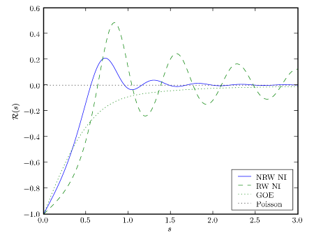
As before, this grows linearly from 11-1. The slope is larger than that of the unmodified RW, but smaller than the slope of the GOE correlations. As shown in figure 7, it rises quickly to positive values.
Refer to caption
Figure 7: Normalized Correlation: NI of normally derived RW.

The expansion for large s𝑠s is:

(s)similar-to𝑠absent\displaystyle\mathcal{R}(s)\sim 2π(2πs)3(925sin(4πs))+5552π(2πs)4cos(4πs)2𝜋superscript2𝜋𝑠39254𝜋𝑠5552𝜋superscript2𝜋𝑠44𝜋𝑠\displaystyle\frac{2}{\pi{(2\pi s)}^{3}}\left(9-25\sin(4\pi s)\right)+\frac{-555}{2\pi{(2\pi s)}^{4}}\cos(4\pi s) (18aeafai)
+12π(2πs)5(692+127898sin(4πs)).12𝜋superscript2𝜋𝑠56921278984𝜋𝑠\displaystyle+\frac{1}{2\pi{(2\pi s)}^{5}}\left(-\frac{69}{2}+\frac{12789}{8}\sin(4\pi s)\right).

(s)𝑠\mathcal{R}(s) decays as s3superscript𝑠3s^{-3}, which is faster than the decay of the correlations for the corresponding RMT ensembles. As in (18w), each asymptotic term has oscillating parts, with frequencies which are multiples of the dominant frequency ωNRW=4πsubscript𝜔NRW4𝜋\omega_{\mathrm{NRW}}=4\pi. As in section 3.1, we find that the oscillations in the nearest neighbour density of the NRW, described in section 2.1, have a frequency which is numerically consistent with half the dominant frequency ω4π𝜔4𝜋\omega\equiv 4\pi.

With the s3superscript𝑠3s^{-3} decay of the correlations, both (s)s𝑠differential-d𝑠\int\mathcal{R}(s)\rmd s and s(s)s𝑠𝑠differential-d𝑠\int s\mathcal{R}(s)\rmd s are finite, so from (18z) it is evident that Σ2superscriptΣ2\Sigma^{2} should increase linearly for large values of L𝐿L. The asymptotic expansion calculated from (18aeafai) is:

Σ2(1+2NRW0)L2NRW1similar-tosuperscriptΣ212subscriptsuperscript0NRW𝐿2subscriptsuperscript1NRW\Sigma^{2}\sim(1+2\mathcal{M}^{0}_{\mathrm{NRW}})L-2\mathcal{M}^{1}_{\mathrm{NRW}} (18aeafaj)

with

NRW0=0(s)s0.2582subscriptsuperscript0NRWsuperscriptsubscript0𝑠differential-d𝑠similar-to0.2582\mathcal{M}^{0}_{\mathrm{NRW}}=\int_{0}^{\infty}\mathcal{R}(s)\rmd s\sim-0.2582

and

NRW1=0s(s)s0.00617.subscriptsuperscript1NRWsuperscriptsubscript0𝑠𝑠differential-d𝑠similar-to0.00617\mathcal{M}^{1}_{\mathrm{NRW}}=\int_{0}^{\infty}s\mathcal{R}(s)\rmd s\sim-0.00617.

As seen in figure 5, the asymptotic variance is larger than RMT ensembles, but smaller than Poisson.

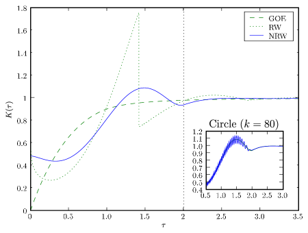
Much in the same way, from (18ac), it is evident that the form factor will now be finite at τ=0𝜏0\tau=0, and will be continuously differentiable for τ>0𝜏0\tau>0. Irregularities appear in second and higher derivatives at multiples of the dominant frequency ωNRWsubscript𝜔NRW\omega_{\mathrm{NRW}} (i.e. τn=nωNRW/(2π)=2nsubscript𝜏𝑛𝑛subscript𝜔NRW2𝜋2𝑛\tau_{n}=n\omega_{\mathrm{NRW}}/(2\pi)=2n). The asymptotic expansion for τ1much-less-than𝜏1\tau\ll 1 is given by:

K(τ)similar-to𝐾𝜏absent\displaystyle K(\tau)\sim (1+2NRW0)+9π2τ2lnτ12subscriptsuperscript0NRW9superscript𝜋2superscript𝜏2𝜏\displaystyle(1+2\mathcal{M}^{0}_{\mathrm{NRW}})+\frac{9}{\pi^{2}}\tau^{2}\ln\tau
+τ2[9π2(γ32+ln2π)(2π)2NRW2]superscript𝜏2delimited-[]9superscript𝜋2𝛾322𝜋superscript2𝜋2subscriptsuperscript2NRW\displaystyle+\tau^{2}\left[\frac{9}{\pi^{2}}(\gamma-\frac{3}{2}+\ln 2\pi)-{(2\pi)}^{2}\mathcal{M}^{2}_{\mathrm{NRW}}\right]

with

NRW2=01s2(s)s+1s2((s)94π4s3)s0.00579subscriptsuperscript2NRWsuperscriptsubscript01superscript𝑠2𝑠differential-d𝑠superscriptsubscript1superscript𝑠2𝑠94superscript𝜋4superscript𝑠3differential-d𝑠similar-to0.00579\mathcal{M}^{2}_{\mathrm{NRW}}=\int_{0}^{1}s^{2}\mathcal{R}(s)\rmd s+\int_{1}^{\infty}s^{2}\left(\mathcal{R}(s)-\frac{9}{4\pi^{4}s^{3}}\right)\rmd s\sim 0.00579

We now have a finite K(0)0.4836similar-to𝐾00.4836K(0)\sim 0.4836. This value is smaller than the K=1𝐾1K=1 of the Poisson distribution, but larger (softer) than the RMT ensembles, for which K(0)=0𝐾00K(0)=0.

Refer to caption
Figure 8: Form factor for the NI of normally derived RW.

4.3 Statistics on a circular arc

The case where the reference curve is a circle can be treated similarly. The amplitude correlations of the monochromatic waves (corrected form for (18aeafag)) can be calculated directly from (18aeafar). It should be noted that the amplitude variance c0=C0(0)subscript𝑐0subscript𝐶00c_{0}=C_{0}(0) remains 12k212superscript𝑘2\frac{1}{2}k^{2} (as for the straight line). However, for any finite k𝑘k, the variance of the derivative (c2subscript𝑐2c_{2}) is different than the value obtained for the straight line, and induces a larger density of intersections.

The corrected density of intersections for the circle is:

ρk~2π=k2+(2κ)22πk2π[1+2(κk)2]𝜌~𝑘2𝜋superscript𝑘2superscript2𝜅22𝜋similar-to𝑘2𝜋delimited-[]12superscript𝜅𝑘2\rho\equiv\frac{\tilde{k}}{2\pi}=\frac{\sqrt{k^{2}+{(2\kappa)}^{2}}}{2\pi}\sim\frac{k}{2\pi}\left[1+2{\left(\frac{\kappa}{k}\right)}^{2}\right]

The O(κ2)Big-Osuperscript𝜅2\Or(\kappa^{2}) increase in density, which is due to curvature, affects the choice of the scaled curve parameter s=ρ(tt)𝑠𝜌𝑡superscript𝑡s=\rho\cdot(t-t^{\prime}) and thus all the correlation formulae. It is convenient to express the resulting statistics in terms of the dimensionless parameter

β=kk~=kr(kr)2+4,𝛽𝑘~𝑘𝑘𝑟superscript𝑘𝑟24\beta=\frac{k}{\tilde{k}}=\frac{kr}{\sqrt{{(kr)}^{2}+4}},

which goes to 1 when kr𝑘𝑟kr\rightarrow\infty. With this, the small s𝑠s expansion of the normalized correlation is:

similar-toabsent\displaystyle\mathcal{R}\sim 1+π28β2(1110β2)s1superscript𝜋28superscript𝛽21110superscript𝛽2𝑠\displaystyle-1+\frac{\pi^{2}}{8}\beta^{2}(11-10\beta^{2})s
+π4576β2(24+357β2820β4+500β6)s3superscript𝜋4576superscript𝛽224357superscript𝛽2820superscript𝛽4500superscript𝛽6superscript𝑠3\displaystyle+\frac{\pi^{4}}{576}\beta^{2}(-24+357\beta^{2}-820\beta^{4}+500\beta^{6})s^{3}

For large values of s𝑠s (the circle is finite, and |s|𝑠|s| can only get values up to 12k~r=(1β2)1/212~𝑘𝑟superscript1superscript𝛽212\frac{1}{2}\tilde{k}r={(1-\beta^{2})}^{-1/2}), the constant dominant frequency ω=4π𝜔4𝜋\omega=4\pi of (18aeafaj) is replaced with a drifting frequency (changing very slowly with s𝑠s)

Ωs=4πβsinc(sk~r),subscriptΩ𝑠4𝜋𝛽sinc𝑠~𝑘𝑟\Omega_{s}=4\pi\beta\mathop{\mathrm{sinc}}\nolimits\!\!\left(\frac{s}{\tilde{k}r}\right),

similar to the situation in section 3.1. However, in the case of the normally derived field, there is another notable difference between the circular and the straight curve. Namely, for any finite value of kr𝑘𝑟kr, we get O(s1)Big-Osuperscript𝑠1\Or(s^{-1}) and O(s2)Big-Osuperscript𝑠2\Or(s^{-2}) terms, which do not appear in the case of a straight line. The leading term of the normalized correlation for s1much-greater-than𝑠1s\gg 1 is

4sin4α[(4β2cos2α1)2(4β2cos2α+1)2sin(Ωss)]1πΩss,4superscript4𝛼delimited-[]superscript4superscript𝛽2superscript2𝛼12superscript4superscript𝛽2superscript2𝛼12subscriptΩ𝑠𝑠1𝜋subscriptΩ𝑠𝑠4\sin^{4}\alpha[{(4\beta^{2}\cos^{2}\alpha-1)}^{2}-{(4\beta^{2}\cos^{2}\alpha+1)}^{2}\sin(\Omega_{s}s)]\cdot\frac{1}{\pi\Omega_{s}s},

where α=πs/(k~r)𝛼𝜋𝑠~𝑘𝑟\alpha=\pi s/(\tilde{k}r) is slowly varying up to π/2𝜋2\pi/2. When we are in the 1sk~rmuch-less-than1𝑠much-less-than~𝑘𝑟1\ll s\ll\tilde{k}r region, α𝛼\alpha is very small, and this term is O(α4)Big-Osuperscript𝛼4\Or(\alpha^{4}). Hence, it vanishes in the straight line limit. The O(s2)Big-Osuperscript𝑠2\Or(s^{-2}) term, contains the frequencies 00, ΩssubscriptΩ𝑠\Omega_{s} and 2Ωs2subscriptΩ𝑠2\Omega_{s}. In the low α𝛼\alpha region, it is O(α2cos(Ωss)(πΩss)2)Big-Osuperscript𝛼2subscriptΩ𝑠𝑠superscript𝜋subscriptΩ𝑠𝑠2\Or\!\!\left(\alpha^{2}\cos(\Omega_{s}s){(\pi\Omega_{s}s)}^{-2}\right) (again, vanishes for the straight line). The O(s3)Big-Osuperscript𝑠3\Or(s^{-3}) term is the first one that does not vanish when α0𝛼0\alpha\rightarrow 0.

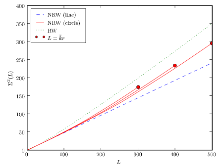
The effect of these terms is manifested by the number variance statistic. In figure 9, the number variance is plotted for three values of kr𝑘𝑟kr. As long as Lk~rmuch-less-than𝐿~𝑘𝑟L\ll\tilde{k}r, the variance stays close to the values corresponding to a straight curve given by (18aeafaj). However, when the angle covered by the segment becomes non negligible, O(α4s1)Big-Osuperscript𝛼4superscript𝑠1\Or(\alpha^{4}s^{-1}) and O(α2s2)Big-Osuperscript𝛼2superscript𝑠2\Or(\alpha^{2}s^{-2}) terms of the correlation become important, and the variance increases above the linear asymptote.
Refer to caption
Figure 9: Number variance for zeros of NRW on a circular curve, for three different values of kr𝑘𝑟kr. The length of the segment is bound by the total length of the circle, marked by circular dots on the plot.

5 Comparison with other fields

The statistics considered above can be evaluated numerically for the nodal intersections of any scalar field with a given reference curve. If a random Gaussian model is given for the field, the techniques demonstrated above can be used to extract the theoretical functions predicted by the model, and those could be compared to the numerical results. This gives a useful tool for verifying statistical models for such systems. For the case of chaotic billiards, the numerical results can be compared to the predictions of random wave models. Also, we can use these statistics to compare other random wave models with the monochromatic random waves. In [14], the field with correlation (7) was compared to the random waves model with respect to special statistics proposed there (which were related to the probability of finding a nodal line inside a reference tube). The nodal intersection statistics provide another way to compare these models.

5.1 The Gaussian short range field

The short range field (7) was chosen so that its short distance behaviour will be the same as that of the monochromatic random wave field, so we expect the average level spacing to be 2π/k2𝜋𝑘\sqrt{2}\pi/k. Substituting the correlation function (7) in (18b), and denoting G=exp(θ2/4)𝐺superscript𝜃24G=\exp(-\theta^{2}/4), θ=kd𝜃𝑘𝑑\theta=kd, we get:

C0=G,C1=12kθcos(α)G,formulae-sequencesubscript𝐶0𝐺subscript𝐶112𝑘𝜃𝛼𝐺\displaystyle C_{0}=G,\quad C_{1}=\frac{1}{2}k\theta\cos(\alpha)G,
C2=12k2[cos(2α)12θ2cos2(α)]Gsubscript𝐶212superscript𝑘2delimited-[]2𝛼12superscript𝜃2superscript2𝛼𝐺\displaystyle C_{2}=\frac{1}{2}k^{2}[\cos(2\alpha)-\frac{1}{2}\theta^{2}\cos^{2}(\alpha)]G

(so c2=k2/2subscript𝑐2superscript𝑘22c_{2}=k^{2}/2 as expected, and θ2πs𝜃2𝜋𝑠\theta\rightarrow\sqrt{2}\pi s as before). The nodal intersections correlation for the straight line becomes:

c^=14θ2112θ212θ2112θ212θ212θ2^𝑐superscript14superscript𝜃21superscript12superscript𝜃212superscript𝜃21superscript12superscript𝜃212superscript𝜃2superscript12superscript𝜃2\displaystyle\hat{c}=\rme^{-\frac{1}{4}\theta^{2}}\frac{1-\rme^{-\frac{1}{2}\theta^{2}}-\frac{1}{2}\theta^{2}}{1-\rme^{-\frac{1}{2}\theta^{2}}-\frac{1}{2}\theta^{2}\rme^{-\frac{1}{2}\theta^{2}}}
(s)=112θ212θ212θ2(112θ2)32(1c^2+c^arcsin(c^))1𝑠1superscript12superscript𝜃212superscript𝜃2superscript12superscript𝜃2superscript1superscript12superscript𝜃2321superscript^𝑐2^𝑐^𝑐1\displaystyle\mathcal{R}(s)=\frac{1-\rme^{-\frac{1}{2}\theta^{2}}-\frac{1}{2}\theta^{2}\rme^{-\frac{1}{2}\theta^{2}}}{{(1-\rme^{-\frac{1}{2}\theta^{2}})}^{\frac{3}{2}}}\left(\sqrt{1-\hat{c}^{2}}+\hat{c}\arcsin(\hat{c})\right)-1 (18aeafak)

The expansion for small s𝑠s is:

1+π24sπ448s3+3π454s4+O(s5),similar-to1superscript𝜋24𝑠superscript𝜋448superscript𝑠33superscript𝜋454superscript𝑠4Big-Osuperscript𝑠5\mathcal{R}\sim-1+\frac{\pi^{2}}{4}s-\frac{\pi^{4}}{48}s^{3}+\frac{\sqrt{3}\pi^{4}}{54}s^{4}+\Or\!\!\left(s^{5}\right),

and for large s𝑠s, it is:

e(πs)2[12(πs)42(πs)2+1]+O(e2(πs)2s8).similar-tosuperscript𝑒superscript𝜋𝑠2delimited-[]12superscript𝜋𝑠42superscript𝜋𝑠21Big-Osuperscript𝑒2superscript𝜋𝑠2superscript𝑠8\mathcal{R}\sim e^{-{(\pi s)}^{2}}\left[\frac{1}{2}{(\pi s)}^{4}-2{(\pi s)}^{2}+1\right]+\Or\!\!\left(e^{-2{(\pi s)}^{2}}s^{8}\right).

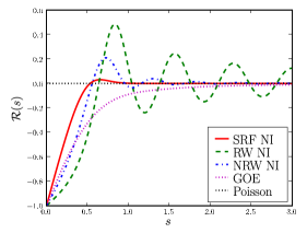
As can be seen in figure 10a, the slope at 0 is higher than that of the GOE, and the correlations decay to 0 faster than all other distributions considered here. Thus, this field has smaller repulsion and it may be considered the closest to the random Poisson distribution.
Refer to caption
(a) Correlations
Refer to caption
(b) Form Factor
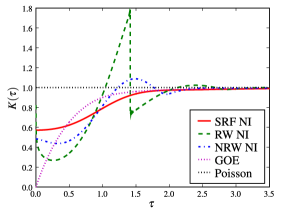
Figure 10: SRF nodal intersections compared to other fields.

The number variance and form factor also reflect this property. Denoting

SRF0=0(s)s0.2141subscriptsuperscript0SRFsuperscriptsubscript0𝑠differential-d𝑠similar-to0.2141\displaystyle\mathcal{M}^{0}_{\mathrm{SRF}}=\int_{0}^{\infty}\mathcal{R}(s)\rmd s\sim-0.2141
SRF1=0s(s)s0.02902subscriptsuperscript1SRFsuperscriptsubscript0𝑠𝑠differential-d𝑠similar-to0.02902\displaystyle\mathcal{M}^{1}_{\mathrm{SRF}}=\int_{0}^{\infty}s\mathcal{R}(s)\rmd s\sim-0.02902
SRF2=0s2(s)s0.00434subscriptsuperscript2SRFsuperscriptsubscript0superscript𝑠2𝑠differential-d𝑠similar-to0.00434\displaystyle\mathcal{M}^{2}_{\mathrm{SRF}}=\int_{0}^{\infty}s^{2}\mathcal{R}(s)\rmd s\sim-0.00434

We find that the asymptotic number variance is linear with coefficient (1+2SRF0)0.5718similar-to12subscriptsuperscript0SRF0.5718(1+2\mathcal{M}^{0}_{\mathrm{SRF}})\sim 0.5718, which is larger than the normally derived random waves (thus closer to Poisson).

The form factor has a smooth form (because (18aeafak) is not oscillatory). The expansion for small τ𝜏\tau is:

K(τ)(1+2SRF0)4π2SRF2τ2similar-to𝐾𝜏12subscriptsuperscript0SRF4superscript𝜋2subscriptsuperscript2SRFsuperscript𝜏2K(\tau)\sim(1+2\mathcal{M}^{0}_{\mathrm{SRF}})-4\pi^{2}\mathcal{M}^{2}_{\mathrm{SRF}}\tau^{2}

We get a relatively large K(0)0.5718similar-to𝐾00.5718K(0)\sim 0.5718, and a quick approach to the limiting value of 1 (which is consistent with the notion that this is closer to the Poisson distribution).

5.2 Chaotic billiards

Eigenfunctions of chaotic billiards provide an ensemble of functions with complex behaviour. In the semiclassical limit, they are well modelled by Gaussian random wave ensembles (the monochromatic random wave ensemble is used to model the eigenfunctions in regions which are far enough from the boundary, and various boundary modified ensembles model the field close to the boundary).

The statistics considered in this paper were evaluated numerically for eigenfunctions of desymmetrized Bunimovich stadium (0.5×10.510.5\times 1 rectangle joined with a quarter of a circle of radius 111) and desymmetrized Sinai billiard (1.2×11.211.2\times 1 rectangle, with a quarter of a circle of radius 0.50.50.5 cut out of one of the corners)—both with Dirichlet boundary conditions. For the Stadium, 1500 eigenfunctions were taken, with wave numbers ranging from k=110𝑘110k=110 to k=165𝑘165k=165. For the Sinai billiard, we used 10000 wave functions, with wave numbers from 350 to 500.

Refer to caption
(a) Stadium billiard
Refer to caption
(b) Sinai billiard
Figure 11: Internal reference curves in the quantum billiards

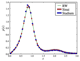
Fixed reference curves were chosen in the interior of the billiards, as shown in figure 11. For each wave function, the sequence of intersections of the nodal lines with these curves was calculated, and normalized to unit average spacing according to the corresponding wavenumber. As shown in figure 12, the nearest neighbour distribution agrees very well with the predictions of the random waves model. The form factor is also very close to the expected curve.
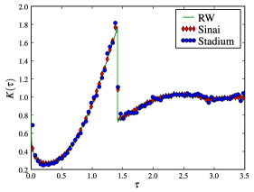
Refer to caption
(a) NN spacing
Refer to caption
(b) Form factor
Figure 12: Billiards: NI with internal line.

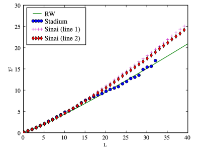
The number variance of nodal intersections on segments of the reference curves is plotted in figure 13. For short segments, the results are close to the predictions of the random waves model, but deviate considerably from this model as we move to segments of large normalized length, especially in the case of the Sinai billiard. This deviation happens when the (unscaled) length of the segment is comparable to the billiard dimensions. On such scales, it seems likely that the geometrical details of the billiard would have an effect on the statistical properties of the wave functions.
Refer to caption
Figure 13: Number variance of NI with segments inside chaotic billiards.

6 Summary

The analytic results obtained for the three Gaussian fields discussed in this paper are summarized in table 1, and compared to their analogues in the well known random matrix and Poisson ensembles. For short distances, the normalized correlation function for all the distributions considered (except of the Poisson distribution) approaches 11-1, so the leading term of 1+(s)1𝑠1+\mathcal{R}(s) is listed, for s=ϵ1𝑠italic-ϵmuch-less-than1s=\epsilon\ll 1. Similarly, the number variance for short intervals is asymptotically LL2𝐿superscript𝐿2L-L^{2} (again, except of the Poisson case), so the leading term of R^2=Σ2(L)L+L2=E[n(n1)]subscript^𝑅2superscriptΣ2𝐿𝐿superscript𝐿2Edelimited-[]𝑛𝑛1\hat{R}_{2}=\Sigma^{2}(L)-L+L^{2}=\mathop{\mathrm{E}}\nolimits[n(n-1)] is listed. (for L=ϵ1𝐿italic-ϵmuch-less-than1L=\epsilon\ll 1, this is also twice the probability for finding two points in the interval). For large distances, we list the leading terms of Σ2superscriptΣ2\Sigma^{2} and \mathcal{R}. For the form factor, we list the “asymptotic rigidity” K(0)𝐾0K(0) (which is directly related to Σ2superscriptΣ2\Sigma^{2} and Δ¯¯Δ\bar{\Delta} in large intervals [20],[23]), the singular frequencies where K(τ)𝐾𝜏K(\tau) or its derivatives diverge and the type of divergence (number of the first diverging derivative) in the first non zero singular frequency.

Table 1: Comparison of NI statistics.
Correlation Form Factor Number Variance
Process
1+(ϵ)1italic-ϵ1+\mathcal{R}(\epsilon) (s1)much-greater-than𝑠1\mathcal{R}(s\gg 1) K(0)𝐾0K(0) Divergences R^2(ϵ)subscript^𝑅2italic-ϵ\hat{R}_{2}(\epsilon) Σ2(L1)superscriptΣ2much-greater-than𝐿1\Sigma^{2}(L\gg 1)
Poisson 111 -0-0\hbox{\phantom{-}}0 111 {} ϵ2superscriptitalic-ϵ2\phantom{0.000}\epsilon^{2} L𝐿\phantom{0.000}L
SRF 2.467ϵ2.467italic-ϵ2.467\epsilon -48.7s4(πs)2-48.7superscript𝑠4superscriptsuperscript𝜋𝑠2\hbox{\phantom{-}}48.7s^{4}\rme^{-{(\pi s)}^{2}} 0.5720.5720.572 {} 0.822ϵ30.822superscriptitalic-ϵ30.822\epsilon^{3} 0.572L0.572𝐿0.572L
NRW 1.234ϵ1.234italic-ϵ1.234\epsilon -0.023s3-0.023superscript𝑠3\hbox{\phantom{-}}0.023s^{-3} 0.4840.4840.484 {2,4,}(3){}^{(3)}\{2,4,\ldots\} 0.411ϵ30.411superscriptitalic-ϵ30.411\epsilon^{3} 0.484L0.484𝐿0.484L
RW 0.617ϵ0.617italic-ϵ0.617\epsilon -0.036s1-0.036superscript𝑠1\hbox{\phantom{-}}0.036s^{-1} \infty {2,22,}(1){}^{(1)}\{\sqrt{2},2\sqrt{2},\ldots\} 0.206ϵ30.206superscriptitalic-ϵ30.206\epsilon^{3} 0.072LlogL0.072𝐿𝐿0.072L\log L
GOE 1.645ϵ1.645italic-ϵ1.645\epsilon 0.101s20.101superscript𝑠2-0.101s^{-2} 00 {1}(4){}^{(4)}\{1\} 0.548ϵ30.548superscriptitalic-ϵ30.548\epsilon^{3} 0.203logL0.203𝐿0.203\log L
GUE 3.290ϵ23.290superscriptitalic-ϵ23.290\epsilon^{2} 0.051s20.051superscript𝑠2-0.051s^{-2} 00 {1}(2){}^{(2)}\{1\} 0.548ϵ40.548superscriptitalic-ϵ40.548\epsilon^{4} 0.101logL0.101𝐿0.101\log L
GSE 11.55ϵ411.55superscriptitalic-ϵ411.55\epsilon^{4} -0.25s1cos(ωs)-0.25superscript𝑠1𝜔𝑠\hbox{\phantom{-}}0.25s^{-1}\cos(\omega s) 00 {1,2}(0){}^{(0)}\{1,2\} 0.770ϵ60.770superscriptitalic-ϵ60.770\epsilon^{6} 0.051logL0.051𝐿0.051\log L

Nonzero values of τ𝜏\tau, for which K(τ)𝐾𝜏K(\tau) or one of its derivatives diverge. The number in parentheses specifies the diverging derivative at the first of these points.

We have seen that

  • Nodal intersections (NI) with a reference curve can be used as a statistical means to obtain insight into the properties of complex networks of lines. The NI statistics of the random wave (RW) model display characteristic behaviour, which is quite different from the statistics of other point processes. Eigenfunctions of chaotic billiards match these statistics well, with some differences on scales comparable to the dimensions of the billiard.

  • For the RW and some other Gaussian models, the two point correlations and other statistics related to it can be derived by analytical means.

  • The nearest neighbour distribution is harder to obtain (since it depends on n𝑛n-point correlations with n3𝑛3n\geq 3). However, numerical evidence suggest that the frequency of oscillations is related to the dominant frequencies calculated for the corresponding two point correlation functions.

This research was initiated as a result of a conversation with Percy Deift, whose interest and help accompanied us throughout the work. Thanks Percy! We would like to acknowledge Sven Gnutzmann for valuable discussion and for the Stadium billiard data, Zeev Rudnick and Mark Dennis for important references. We thank Holger Schanz for the Sinai billiard data, and Yehonatan Elon for careful reading of the text and useful comments. The work was supported by the Minerva Center for non-linear Physics and the Einstein (Minerva) Center at the Weizmann Institute, and by grants from the GIF (grant I–808–228.14/2003), and EPSRC (grant GR/T06872/01.) and a Minerva grant.

Appendix A Derivation of the zeros correlation from amplitude statistics

In section 2.4, the correlation of the zeros of a Gaussian random function on a curve was expressed in terms of the Fourier integral (15):

ρρ=14π4ξηξηη2η2ξf(1ηf˙)ξf(1ηf˙)delimited-⟨⟩𝜌superscript𝜌delimited-⟨⟩14superscript𝜋4differential-d𝜉differential-d𝜂differential-dsuperscript𝜉differential-dsuperscript𝜂superscript𝜂2superscript𝜂2superscript𝜉𝑓1superscript𝜂˙𝑓superscriptsuperscript𝜉superscript𝑓1superscriptsuperscript𝜂superscript˙𝑓\langle\rho\rho^{\prime}\rangle=\left\langle\frac{1}{4\pi^{4}}\int\frac{\rmd\xi\,\rmd\eta\,\rmd\xi^{\prime}\,\rmd\eta^{\prime}}{\eta^{2}\eta^{\prime 2}}\rme^{\rmi\xi f}(1-\rme^{\rmi\eta\dot{f}})\rme^{\rmi\xi^{\prime}f^{\prime}}(1-\rme^{\rmi\eta^{\prime}\dot{f}^{\prime}})\right\rangle

We note that the integrand contains four terms of the form exp(ivif)bold-⋅𝑖subscriptvif\exp(i\bi{v}_{i}\cdot\bi{f}), with

vi{(𝝃,𝝃,0,0),(𝝃,𝝃,𝜼,0),(𝝃,𝝃,0,𝜼),(𝝃,𝝃,𝜼,𝜼)},subscriptvi𝝃superscript𝝃bold-′00𝝃superscript𝝃bold-′𝜼0𝝃superscript𝝃bold-′0superscript𝜼bold-′𝝃superscript𝝃bold-′𝜼superscript𝜼bold-′\displaystyle\bi{v}_{i}\in\{(\xi,\xi^{\prime},0,0),(\xi,\xi^{\prime},\eta,0),(\xi,\xi^{\prime},0,\eta^{\prime}),(\xi,\xi^{\prime},\eta,\eta^{\prime})\},
andf=(f,f,f˙,f˙).andffsuperscriptfbold-′bold-˙fsuperscriptbold-˙fbold-′\displaystyle\mathrm{and}\quad\bi{f}=(f,f^{\prime},\dot{f},\dot{f}^{\prime}).

If we use (13) to evaluate the statistical average, these terms are replaced by exp(12viTMvi)12superscriptsubscriptviTMsubscriptvi\exp\!\!\left(-\frac{1}{2}\bi{v_{i}}^{T}M\bi{v_{i}}\right), where M𝑀M is the covariance matrix of ff\bi{f}, given in (16). To continue, we first integrate the ξ𝜉\xi and ξsuperscript𝜉\xi^{\prime} coordinates. To separate them out, we use a simple block matrix identity.

For any pair of column vectors x,ynxysuperscriptn\bi{x},\bi{y}\in\mathbb{R}^{n} and three n×n𝑛𝑛n\times n matrices A,B,C𝐴𝐵𝐶A,B,C, where A𝐴A and B𝐵B are symmetric and A𝐴A is non-singular, the following identity can be simply derived:

(xTyT)(ACCTB)(xy)=(xT+y~T)A(x+y~)+yTB~ysuperscriptxTsuperscriptyTACsuperscriptCTBxysuperscriptxTsuperscriptbold-~yTAxbold-~ysuperscriptyTbold-~By(\bi{x}^{T}\bi{y}^{T})\left(\begin{array}[]{cc}A&C\\ C^{T}&B\end{array}\right)\left(\begin{array}[]{c}\bi{x}\\ \bi{y}\end{array}\right)=(\bi{x}^{T}+\tilde{\bi{y}}^{T})A(\bi{x}+\tilde{\bi{y}})+\bi{y}^{T}\tilde{B}\bi{y} (18aeafal)

where B~=BCTA1C~𝐵𝐵superscript𝐶𝑇superscript𝐴1𝐶\tilde{B}=B-C^{T}A^{-1}C and y~=A1Cy~ysuperscript𝐴1𝐶y\tilde{\bi{y}}=A^{-1}C\bi{y}.

In addition, using the same notation, one can also deduce the determinant identity

det(ACCTB)=detAdetB~,𝐴𝐶superscript𝐶𝑇𝐵𝐴~𝐵\det\left(\begin{array}[]{cc}A&C\\ C^{T}&B\end{array}\right)=\det A\det\tilde{B}, (18aeafam)

which we shall use below.

Applying (18aeafal) to the four terms, with viT=(xT,yiT)superscriptsubscriptvi𝑇superscriptxTsuperscriptsubscriptyiT{\bi{v}_{i}}^{T}=(\bi{x}^{T},{\bi{y}_{i}}^{T}) (i.e. xT=(𝝃,𝝃)superscriptxT𝝃superscript𝝃bold-′\bi{x}^{T}=(\xi,\xi^{\prime}) and yiT{(0,0),(η,0),(0,η),(η,η)}superscriptsubscriptyi𝑇00𝜂00superscript𝜂𝜂superscript𝜂{\bi{y}_{i}}^{T}\in\{(0,0),(\eta,0),(0,\eta^{\prime}),(\eta,\eta^{\prime})\}), the xx\bi{x} dependent integration for each of the four terms reduces to the usual Gaussian form:

ξξ12(xT+y~iT)A(x+y~i)=2πdetAdifferential-d𝜉differential-dsuperscript𝜉superscript12superscriptxTsuperscriptsubscriptbold-~yiTAxsubscriptbold-~yi2𝜋𝐴\int\rmd\xi\rmd\xi^{\prime}\rme^{-\frac{1}{2}(\bi{x}^{T}+{\tilde{\bi{y}}_{i}}^{T})A(\bi{x}+\tilde{\bi{y}}_{i})}=\frac{2\pi}{\sqrt{\det A}}

This does not depend on yy\bi{y} and therefore contributes a constant multiplicative factor. The remaining integral assumes the following form:

ηηη2η2(112aη212bη2+12y2TB~y2)superscriptsubscriptdifferential-d𝜂differential-dsuperscript𝜂superscript𝜂2superscript𝜂21superscript12𝑎superscript𝜂2superscript12𝑏superscript𝜂2superscript12superscriptsubscripty2𝑇~𝐵subscripty2\int\!\!\!\int_{-\infty}^{\infty}\frac{\rmd\eta\rmd\eta^{\prime}}{\eta^{2}\eta^{\prime 2}}\left(1-\rme^{-\frac{1}{2}a\eta^{2}}-\rme^{-\frac{1}{2}b\eta^{\prime 2}}+\rme^{-\frac{1}{2}{\bi{y}_{2}}^{T}\tilde{B}\bi{y}_{2}}\right)

(using a𝑎a,b𝑏b and c𝑐c for the matrix elements of B~~𝐵\tilde{B}).

This can be rewritten as I1+I2subscript𝐼1subscript𝐼2I_{1}+I_{2}, where

I1=ηηη2η2(112aη2)(112bη2)=2πabsubscript𝐼1superscriptsubscriptdifferential-d𝜂differential-dsuperscript𝜂superscript𝜂2superscript𝜂21superscript12𝑎superscript𝜂21superscript12𝑏superscript𝜂22𝜋𝑎𝑏I_{1}=\int\!\!\!\int_{-\infty}^{\infty}\frac{\rmd\eta\rmd\eta^{\prime}}{\eta^{2}\eta^{\prime 2}}(1-\rme^{-\frac{1}{2}a\eta^{2}})(1-\rme^{-\frac{1}{2}b\eta^{\prime 2}})=2\pi\sqrt{ab}

and

I2=ηηη2η212(aη2+bη2)(cηη1)subscript𝐼2superscriptsubscriptdifferential-d𝜂differential-dsuperscript𝜂superscript𝜂2superscript𝜂2superscript12𝑎superscript𝜂2𝑏superscript𝜂2superscript𝑐𝜂superscript𝜂1I_{2}=\int\!\!\!\int_{-\infty}^{\infty}\frac{\rmd\eta\rmd\eta^{\prime}}{\eta^{2}\eta^{\prime 2}}\rme^{-\frac{1}{2}(a\eta^{2}+b\eta^{\prime 2})}(\rme^{-c\eta\eta^{\prime}}-1)

I2subscript𝐼2I_{2} is not well defined, but taking the Cauchy Principal Value for the integrals, anti-symmetric integrands do not contribute. After symmetrization and change of integration variables, we get:

I2=abxyx2y212(x2+y2)[cosh(c^xy)1]subscript𝐼2𝑎𝑏superscriptsubscriptdifferential-d𝑥differential-d𝑦superscript𝑥2superscript𝑦2superscript12superscript𝑥2superscript𝑦2delimited-[]^𝑐𝑥𝑦1I_{2}=\sqrt{ab}\int\!\!\!\int_{-\infty}^{\infty}\frac{\rmd x\rmd y}{x^{2}y^{2}}\rme^{-\frac{1}{2}(x^{2}+y^{2})}\left[\cosh(\hat{c}xy)-1\right]

with c^c/ab^𝑐𝑐𝑎𝑏\hat{c}\equiv c/\sqrt{ab}. One way to solve this integral is to derive the expression by c^^𝑐\hat{c} twice, and integrate back after the x𝑥x and y𝑦y integrations. Another way is to express f(xy)(xy)2[cosh(c^xy)1]𝑓𝑥𝑦superscript𝑥𝑦2delimited-[]^𝑐𝑥𝑦1f(xy)\equiv{(xy)}^{-2}[\cosh(\hat{c}xy)-1] as a power series in (xy)2superscript𝑥𝑦2{(xy)}^{2}, and integrate term by term (each term becomes a square of a simple Gaussian moment). Either way, for any |c^|<1^𝑐1|\hat{c}|<1, we get

I2=2πab[1+1c^2+c^arcsinc^],subscript𝐼22𝜋𝑎𝑏delimited-[]11superscript^𝑐2^𝑐^𝑐I_{2}=2\pi\sqrt{ab}\left[-1+\sqrt{1-\hat{c}^{2}}+\hat{c}\arcsin\hat{c}\right],

To show that the convergence condition |c^|<1^𝑐1|\hat{c}|<1 holds, we note that

|c^|<1detB~=abc2>0.^𝑐1~𝐵𝑎𝑏superscript𝑐20|\hat{c}|<1\Leftrightarrow\det\tilde{B}=ab-c^{2}>0.

However, from (18aeafam) we have detM=detAdetB~𝑀𝐴~𝐵\det M=\det A\det\tilde{B}. Since both A𝐴A and M𝑀M are covariance matrices, they are positive definite, and their determinant must be positive for any non-degenerate case. This can only be consistent if detB~~𝐵\det\tilde{B} is positive too.

Inserting I1subscript𝐼1I_{1} and I2subscript𝐼2I_{2} into the expression for the normalized correlation we find (17)

(t,t)=c0c2a(detA)3/2(1c^2+c^arcsin(c^))1𝑡superscript𝑡subscript𝑐0subscript𝑐2𝑎superscript𝐴321superscript^𝑐2^𝑐^𝑐1\mathcal{R}(t,t^{\prime})=\frac{c_{0}}{c_{2}}\frac{a}{{(\det A)}^{3/2}}\left(\sqrt{1-\hat{c}^{2}}+\hat{c}\arcsin(\hat{c})\right)-1

Appendix B Calculating the amplitude correlations for the normal derivative of a Gaussian field

When the investigated field is translationally invariant and isotropic, the correlation functions C0subscript𝐶0C_{0}, C1subscript𝐶1C_{1} and C2subscript𝐶2C_{2} for the “normally derived” function g(t)=n(t)𝝍(r(t))𝑔𝑡bold-⋅ntbold-▽𝝍rtg(t)=\bi{n}(t)\cdot\bi{\triangledown}\psi(\bi{r}(t)) can be calculated in terms of the curve parameters and reduced correlation function G(d)𝐺𝑑G(d). The derivation is straightforward but tedious, and follows the same mechanism used in section 2.3 and section 4.1. In this section we recite the main steps and results.

As in previous sections, we start by using linearity to move the derivatives out of the statistical average, getting (18ad) for the first correlation function C0subscript𝐶0C_{0}. This expression involves second order partial derivatives of the basic correlation ψψdelimited-⟨⟩𝜓superscript𝜓\langle\psi\psi^{\prime}\rangle, so the expressions for C1subscript𝐶1C_{1} and C2subscript𝐶2C_{2} involve third and fourth order partial derivatives correspondingly.

Using shorthand notation where tagged parameters refer to values at tsuperscript𝑡t^{\prime}, i/risubscript𝑖subscript𝑟𝑖\partial_{i}\equiv\partial/\partial r_{i} and i/risubscriptsuperscript𝑖subscriptsuperscript𝑟𝑖{\partial^{\prime}}_{i}\equiv\partial/\partial{r^{\prime}}_{i}, we have

C0=subscript𝐶0absent\displaystyle C_{0}= i,jninjijG(|rr|)subscript𝑖𝑗subscript𝑛𝑖subscriptsuperscript𝑛𝑗subscript𝑖subscriptsuperscript𝑗𝐺rsuperscriptrbold-′\displaystyle\sum_{i,j}n_{i}{n^{\prime}}_{j}\partial_{i}{\partial^{\prime}}_{j}G(|\bi{r}-\bi{r}^{\prime}|)
C1=subscript𝐶1absent\displaystyle C_{1}= i,jtninjijGsubscript𝑖𝑗subscriptsuperscript𝑡subscript𝑛𝑖subscriptsuperscript𝑛𝑗subscript𝑖subscriptsuperscript𝑗𝐺\displaystyle\sum_{i,j}{\partial^{\prime}}_{t}n_{i}{n^{\prime}}_{j}\partial_{i}{\partial^{\prime}}_{j}G
C2=subscript𝐶2absent\displaystyle C_{2}= i,jttninjijGsubscript𝑖𝑗subscript𝑡subscriptsuperscript𝑡subscript𝑛𝑖subscriptsuperscript𝑛𝑗subscript𝑖subscriptsuperscript𝑗𝐺\displaystyle\sum_{i,j}\partial_{t}{\partial^{\prime}}_{t}n_{i}{n^{\prime}}_{j}\partial_{i}{\partial^{\prime}}_{j}G (18aeafan)

The derivatives of nn\bi{n} in these expressions can be evaluated using Frenet formula tn=𝜿r˙subscript𝑡n𝜿bold-˙r\partial_{t}\bi{n}=-\kappa\dot{\bi{r}} (where κ𝜅\kappa is the curvature at t𝑡t), and the partial derivatives of G𝐺G can be expressed in terms of derivatives with respect to d𝑑d (Gsuperscript𝐺G^{\prime},G′′superscript𝐺′′G^{\prime\prime},G(3)superscript𝐺3G^{(3)},G(4)superscript𝐺4G^{(4)}) and the distance vector dd\bi{d}.

First, we calculate the partial derivatives of G𝐺G using the following rules for derivatives of the distance d|d|𝑑dd\equiv|\bi{d}| and direction vector d^d/d^ddd\hat{\bi{d}}\equiv\bi{d}/d (where d=rrdrsuperscriptrbold-′\bi{d}=\bi{r}-\bi{r^{\prime}}):

id=id=d^isubscript𝑖𝑑subscriptsuperscript𝑖𝑑subscript^𝑑𝑖\displaystyle\partial_{i}d=-{\partial^{\prime}}_{i}d=\hat{d}_{i}
id^j=id^j=1d(δijd^id^j)subscript𝑖subscript^𝑑𝑗subscriptsuperscript𝑖subscript^𝑑𝑗1𝑑subscript𝛿𝑖𝑗subscript^𝑑𝑖subscript^𝑑𝑗\displaystyle\partial_{i}\hat{d}_{j}=-{\partial^{\prime}}_{i}\hat{d}_{j}=\frac{1}{d}\left(\delta_{ij}-\hat{d}_{i}\hat{d}_{j}\right)

To express the results in a manifestly symmetric way, we define di1,i2,,iN[k]subscriptsuperscript𝑑delimited-[]𝑘subscript𝑖1subscript𝑖2subscript𝑖𝑁d^{[k]}_{i_{1},i_{2},\ldots,i_{N}}, the “N𝑁N dimensional symmetric direction tensor of degeneracy k𝑘k” as the symmetrized product of k𝑘k Kronecker deltas and N2k𝑁2𝑘N-2k direction vectors d^^d\hat{\bi{d}}. Specifically:

dij[0]=subscriptsuperscript𝑑delimited-[]0𝑖𝑗absent\displaystyle d^{[0]}_{ij}= d^id^j,dij[1]=δijsubscript^𝑑𝑖subscript^𝑑𝑗subscriptsuperscript𝑑delimited-[]1𝑖𝑗subscript𝛿𝑖𝑗\displaystyle\hat{d}_{i}\hat{d}_{j},\quad d^{[1]}_{ij}=\delta_{ij}
dijk[1]=subscriptsuperscript𝑑delimited-[]1𝑖𝑗𝑘absent\displaystyle d^{[1]}_{ijk}= δijd^k+δikd^j+δjkd^isubscript𝛿𝑖𝑗subscript^𝑑𝑘subscript𝛿𝑖𝑘subscript^𝑑𝑗subscript𝛿𝑗𝑘subscript^𝑑𝑖\displaystyle\delta_{ij}\hat{d}_{k}+\delta_{ik}\hat{d}_{j}+\delta_{jk}\hat{d}_{i}
dijkl[1]=subscriptsuperscript𝑑delimited-[]1𝑖𝑗𝑘𝑙absent\displaystyle d^{[1]}_{ijkl}= δijd^kd^l+δikd^jd^l+δild^jd^k+subscript𝛿𝑖𝑗subscript^𝑑𝑘subscript^𝑑𝑙subscript𝛿𝑖𝑘subscript^𝑑𝑗subscript^𝑑𝑙limit-fromsubscript𝛿𝑖𝑙subscript^𝑑𝑗subscript^𝑑𝑘\displaystyle\delta_{ij}\hat{d}_{k}\hat{d}_{l}+\delta_{ik}\hat{d}_{j}\hat{d}_{l}+\delta_{il}\hat{d}_{j}\hat{d}_{k}+
δjkd^id^l+δjld^id^k+δkld^id^jsubscript𝛿𝑗𝑘subscript^𝑑𝑖subscript^𝑑𝑙subscript𝛿𝑗𝑙subscript^𝑑𝑖subscript^𝑑𝑘subscript𝛿𝑘𝑙subscript^𝑑𝑖subscript^𝑑𝑗\displaystyle\delta_{jk}\hat{d}_{i}\hat{d}_{l}+\delta_{jl}\hat{d}_{i}\hat{d}_{k}+\delta_{kl}\hat{d}_{i}\hat{d}_{j}
dijkl[2]=subscriptsuperscript𝑑delimited-[]2𝑖𝑗𝑘𝑙absent\displaystyle d^{[2]}_{ijkl}= δijδkl+δikδjl+δilδjksubscript𝛿𝑖𝑗subscript𝛿𝑘𝑙subscript𝛿𝑖𝑘subscript𝛿𝑗𝑙subscript𝛿𝑖𝑙subscript𝛿𝑗𝑘\displaystyle\delta_{ij}\delta_{kl}+\delta_{ik}\delta_{jl}+\delta_{il}\delta_{jk}

We also introduce the notation G[n]superscript𝐺delimited-[]𝑛G^{[n]} for the specific combinations of derivatives of G𝐺G up to order n𝑛n, which satisfy the following recurrence relations333 These relations are almost identical to the Bessel recurrence relations. Hence, for the case where G(d)=J0(kd)𝐺𝑑subscript𝐽0𝑘𝑑G(d)=J_{0}(kd), we get G[n]=(k)nJn(kd)superscript𝐺delimited-[]𝑛superscript𝑘𝑛subscript𝐽𝑛𝑘𝑑G^{[n]}={(-k)}^{n}J_{n}(kd) :

G[0](d)=G(d)superscript𝐺delimited-[]0𝑑𝐺𝑑\displaystyle G^{[0]}(d)=G(d)
G[n+1](d)=G[n](d)ndG[n](d)superscript𝐺delimited-[]𝑛1𝑑superscriptsuperscript𝐺delimited-[]𝑛𝑑𝑛𝑑superscript𝐺delimited-[]𝑛𝑑\displaystyle G^{[n+1]}(d)={G^{[n]}}^{\prime}(d)-\frac{n}{d}G^{[n]}(d)

Specifically, we have:

G[1]=Gsuperscript𝐺delimited-[]1superscript𝐺\displaystyle G^{[1]}=G^{\prime}
G[2]=G′′1dGsuperscript𝐺delimited-[]2superscript𝐺′′1𝑑superscript𝐺\displaystyle G^{[2]}=G^{\prime\prime}-\frac{1}{d}G^{\prime}
G[3]=G(3)3dG′′+3d2Gsuperscript𝐺delimited-[]3superscript𝐺33𝑑superscript𝐺′′3superscript𝑑2superscript𝐺\displaystyle G^{[3]}=G^{(3)}-\frac{3}{d}G^{\prime\prime}+\frac{3}{d^{2}}G^{\prime}
G[4]=G(4)6dG(3)+15d2G′′15d3Gsuperscript𝐺delimited-[]4superscript𝐺46𝑑superscript𝐺315superscript𝑑2superscript𝐺′′15superscript𝑑3superscript𝐺\displaystyle G^{[4]}=G^{(4)}-\frac{6}{d}G^{(3)}+\frac{15}{d^{2}}G^{\prime\prime}-\frac{15}{d^{3}}G^{\prime}

With these notations, the partial derivatives of G𝐺G are given by:

iG=G[1]di[0]subscript𝑖𝐺superscript𝐺delimited-[]1superscriptsubscript𝑑𝑖delimited-[]0\displaystyle\partial_{i}G=G^{[1]}d_{i}^{[0]}
ijG=G[2]dij[0]+1dG[1]dij[1]subscript𝑖subscript𝑗𝐺superscript𝐺delimited-[]2superscriptsubscript𝑑𝑖𝑗delimited-[]01𝑑superscript𝐺delimited-[]1superscriptsubscript𝑑𝑖𝑗delimited-[]1\displaystyle\partial_{i}\partial_{j}G=G^{[2]}d_{ij}^{[0]}+\frac{1}{d}G^{[1]}d_{ij}^{[1]}
ijkG=G[3]dijk[0]+1dG[2]dijk[1]subscript𝑖subscript𝑗subscript𝑘𝐺superscript𝐺delimited-[]3superscriptsubscript𝑑𝑖𝑗𝑘delimited-[]01𝑑superscript𝐺delimited-[]2superscriptsubscript𝑑𝑖𝑗𝑘delimited-[]1\displaystyle\partial_{i}\partial_{j}\partial_{k}G=G^{[3]}d_{ijk}^{[0]}+\frac{1}{d}G^{[2]}d_{ijk}^{[1]}
ijklG=G[4]dijkl[0]+1dG[3]dijkl[1]+1d2G[2]dijkl[2]subscript𝑖subscript𝑗subscript𝑘subscript𝑙𝐺superscript𝐺delimited-[]4superscriptsubscript𝑑𝑖𝑗𝑘𝑙delimited-[]01𝑑superscript𝐺delimited-[]3superscriptsubscript𝑑𝑖𝑗𝑘𝑙delimited-[]11superscript𝑑2superscript𝐺delimited-[]2superscriptsubscript𝑑𝑖𝑗𝑘𝑙delimited-[]2\displaystyle\partial_{i}\partial_{j}\partial_{k}\partial_{l}G=G^{[4]}d_{ijkl}^{[0]}+\frac{1}{d}G^{[3]}d_{ijkl}^{[1]}+\frac{1}{d^{2}}G^{[2]}d_{ijkl}^{[2]}

Substituting these in (18aeafan), we get

C0subscript𝐶0\displaystyle C_{0} =i,jninj(G[2]dij[0]+1dG[1]dij[1])absentsubscript𝑖𝑗subscript𝑛𝑖subscriptsuperscript𝑛𝑗superscript𝐺delimited-[]2superscriptsubscript𝑑𝑖𝑗delimited-[]01𝑑superscript𝐺delimited-[]1superscriptsubscript𝑑𝑖𝑗delimited-[]1\displaystyle=\sum_{i,j}-n_{i}{n^{\prime}}_{j}(G^{[2]}d_{ij}^{[0]}+\frac{1}{d}G^{[1]}d_{ij}^{[1]}) (18aeafao)
=(nd^)(nd^)G[2](nn)1dG[1]absentbold-⋅nbold-^dbold-⋅superscriptnbold-′bold-^dsuperscriptGdelimited-[]2bold-⋅nsuperscriptnbold-′1dsuperscriptGdelimited-[]1\displaystyle=-(\bi{n}\cdot\hat{\bi{d}})(\bi{n}^{\prime}\cdot\hat{\bi{d}})G^{[2]}-(\bi{n}\cdot\bi{n}^{\prime})\frac{1}{d}G^{[1]}

which is equivalent to (18ad). Similarly,

C1subscript𝐶1\displaystyle C_{1} =\displaystyle= i,jκnir˙jijG+i,j,kninjr˙kijkGsubscript𝑖𝑗superscript𝜅subscript𝑛𝑖subscriptsuperscript˙𝑟𝑗subscript𝑖subscript𝑗𝐺subscript𝑖𝑗𝑘subscript𝑛𝑖subscriptsuperscript𝑛𝑗subscriptsuperscript˙𝑟𝑘subscript𝑖subscript𝑗subscript𝑘𝐺\displaystyle\sum_{i,j}\kappa^{\prime}n_{i}{\dot{r}^{\prime}}_{j}\partial_{i}\partial_{j}G+\sum_{i,j,k}n_{i}{n^{\prime}}_{j}{\dot{r}^{\prime}}_{k}\partial_{i}\partial_{j}\partial_{k}G (18aeafap)
=\displaystyle= κ[(nd^)(r˙d^)G[2]+(nr˙)1dG[1]]superscript𝜅delimited-[]nbold-^dsuperscriptbold-˙rbold-′bold-^dsuperscriptGdelimited-[]2nsuperscriptbold-˙rbold-′1dsuperscriptGdelimited-[]1\displaystyle\kappa^{\prime}\left[(\bi{n}\hat{\bi{d}})(\dot{\bi{r}}^{\prime}\hat{\bi{d}})G^{[2]}+(\bi{n}\dot{\bi{r}}^{\prime})\frac{1}{d}G^{[1]}\right]
+(nd^)(nd^)(r˙d^)G[3]+1d[(nn)(r˙d^)+(nr˙)(nd^)]G[2]nbold-^dsuperscriptnbold-′bold-^dsuperscriptbold-˙rbold-′bold-^dsuperscriptGdelimited-[]31ddelimited-[]nsuperscriptnbold-′superscriptbold-˙rbold-′bold-^dnsuperscriptbold-˙rbold-′superscriptnbold-′bold-^dsuperscriptGdelimited-[]2\displaystyle+(\bi{n}\hat{\bi{d}})(\bi{n}^{\prime}\hat{\bi{d}})(\dot{\bi{r}}^{\prime}\hat{\bi{d}})G^{[3]}+\frac{1}{d}\left[(\bi{n}\bi{n}^{\prime})(\dot{\bi{r}}^{\prime}\hat{\bi{d}})+(\bi{n}\dot{\bi{r}}^{\prime})(\bi{n}^{\prime}\hat{\bi{d}})\right]G^{[2]}

and, defining d~=κn𝜿n~dsuperscript𝜅n𝜿superscriptnbold-′\tilde{\bi{d}}=\kappa^{\prime}\bi{n}-\kappa\bi{n}^{\prime}, we get

C2subscript𝐶2\displaystyle C_{2} =\displaystyle= κκr˙ir˙jijG+d~ir˙jr˙kijkG+ninjr˙kr˙lijklG𝜅superscript𝜅subscript˙𝑟𝑖subscriptsuperscript˙𝑟𝑗subscript𝑖𝑗𝐺subscript~𝑑𝑖subscript˙𝑟𝑗subscriptsuperscript˙𝑟𝑘subscript𝑖𝑗𝑘𝐺subscript𝑛𝑖subscriptsuperscript𝑛𝑗subscript˙𝑟𝑘subscriptsuperscript˙𝑟𝑙subscript𝑖𝑗𝑘𝑙𝐺\displaystyle-\kappa\kappa^{\prime}\dot{r}_{i}{\dot{r}^{\prime}}_{j}\partial_{ij}G+\tilde{d}_{i}\dot{r}_{j}{\dot{r}^{\prime}}_{k}\partial_{ijk}G+n_{i}{n^{\prime}}_{j}\dot{r}_{k}{\dot{r}^{\prime}}_{l}\partial_{ijkl}G (18aeafaq)
=\displaystyle= κκ[(r˙d^)(r˙d^)G[2]+(r˙r˙)1dG[1]]𝜅superscript𝜅delimited-[]˙r^dsuperscript˙r^dsuperscript𝐺delimited-[]2˙rsuperscript˙r1𝑑superscript𝐺delimited-[]1\displaystyle-\kappa\kappa^{\prime}\left[(\dot{\bi{r}}\hat{\bi{d}})(\dot{\bi{r}}^{\prime}\hat{\bi{d}})G^{[2]}+(\dot{\bi{r}}\dot{\bi{r}}^{\prime})\frac{1}{d}G^{[1]}\right]
+(d~d^)(r˙d^)(r˙d^)G[3]~d^d˙r^dsuperscript˙r^dsuperscript𝐺delimited-[]3\displaystyle+(\tilde{\bi{d}}\hat{\bi{d}})(\dot{\bi{r}}\hat{\bi{d}})(\dot{\bi{r}}^{\prime}\hat{\bi{d}})G^{[3]}
+[(d~r˙)(r˙d^)+(d~r˙)(r˙d^)+(d~d^)(r˙r˙)]1dG[2]delimited-[]~d˙rsuperscript˙r^d~dsuperscript˙r˙r^d~d^d˙rsuperscript˙r1𝑑superscript𝐺delimited-[]2\displaystyle\qquad+\left[(\tilde{\bi{d}}\dot{\bi{r}})(\dot{\bi{r}}^{\prime}\hat{\bi{d}})+(\tilde{\bi{d}}\dot{\bi{r}}^{\prime})(\dot{\bi{r}}\hat{\bi{d}})+(\tilde{\bi{d}}\hat{\bi{d}})(\dot{\bi{r}}\dot{\bi{r}}^{\prime})\right]\frac{1}{d}G^{[2]}
+(nd^)(nd^)(r˙d^)(r˙d^)G[4]nbold-^dsuperscriptnbold-′bold-^dbold-˙rbold-^dsuperscriptbold-˙rbold-′bold-^dsuperscriptGdelimited-[]4\displaystyle+(\bi{n}\hat{\bi{d}})(\bi{n}^{\prime}\hat{\bi{d}})(\dot{\bi{r}}\hat{\bi{d}})(\dot{\bi{r}}^{\prime}\hat{\bi{d}})G^{[4]}
+[(nd^)(nd^)(r˙r˙)+(nd^)(r˙d^)(r˙n)\displaystyle\qquad+\left[(\bi{n}\hat{\bi{d}})(\bi{n}^{\prime}\hat{\bi{d}})(\dot{\bi{r}}\dot{\bi{r}}^{\prime})+(\bi{n}\hat{\bi{d}})(\dot{\bi{r}}^{\prime}\hat{\bi{d}})(\dot{\bi{r}}\bi{n}^{\prime})\right.
+(nd^)(r˙d^)(nr˙)+(r˙d^)(r˙d^)(nn)]1dG[3]\displaystyle\qquad\quad\left.+(\bi{n}^{\prime}\hat{\bi{d}})(\dot{\bi{r}}\hat{\bi{d}})(\bi{n}\dot{\bi{r}}^{\prime})+(\dot{\bi{r}}\hat{\bi{d}})(\dot{\bi{r}}^{\prime}\hat{\bi{d}})(\bi{n}\bi{n}^{\prime})\right]\frac{1}{d}G^{[3]}
+[(nn)(r˙r˙)+(nr˙)(r˙n)]1d2G[2]delimited-[]nsuperscriptnbold-′bold-˙rsuperscriptbold-˙rbold-′nsuperscriptbold-˙rbold-′bold-˙rsuperscriptnbold-′1superscript𝑑2superscript𝐺delimited-[]2\displaystyle\qquad+\left[(\bi{n}\bi{n}^{\prime})(\dot{\bi{r}}\dot{\bi{r}}^{\prime})+(\bi{n}\dot{\bi{r}}^{\prime})(\dot{\bi{r}}\bi{n}^{\prime})\right]\frac{1}{d^{2}}G^{[2]}

For the case where the curve is a circle, equations (18aeafao)–(18aeafaq) can be much simplified. Denoting α=12κ(tt)𝛼12𝜅𝑡superscript𝑡\alpha=\frac{1}{2}\kappa(t-t^{\prime}) as in section 3, the following identities hold:

κ=κ,d=2κsinα,d~=2κsinαd^formulae-sequence𝜅superscript𝜅formulae-sequence𝑑2𝜅𝛼~d2𝜅𝛼^d\displaystyle\kappa=\kappa^{\prime},\quad d=\frac{2}{\kappa}\sin\alpha,\quad\tilde{\bi{d}}=-2\kappa\sin\alpha\hat{\bi{d}}
d^r˙=d^r˙=cos(α),d^n=d^n=𝐬𝐢𝐧(𝜶)formulae-sequence^d˙r^dsuperscript˙r𝛼^dnbold-⋅bold-^dsuperscriptnbold-′𝜶\displaystyle\hat{\bi{d}}\cdot\dot{\bi{r}}=\hat{\bi{d}}\cdot\dot{\bi{r}}^{\prime}=\cos(\alpha),\quad\hat{\bi{d}}\cdot\bi{n}=-\hat{\bi{d}}\cdot\bi{n}^{\prime}=-\sin(\alpha)
nn=r˙r˙=𝐜𝐨𝐬(2𝜶),r˙n=r˙n=𝐬𝐢𝐧(2𝜶)formulae-sequencebold-⋅nsuperscriptnbold-′bold-⋅bold-˙rsuperscriptbold-˙rbold-′2𝜶bold-⋅bold-˙rsuperscriptnbold-′bold-⋅superscriptbold-˙rbold-′n2𝜶\displaystyle\bi{n}\cdot\bi{n}^{\prime}=\dot{\bi{r}}\cdot\dot{\bi{r}}^{\prime}=\cos(2\alpha),\quad\dot{\bi{r}}\cdot\bi{n}^{\prime}=-\dot{\bi{r}}^{\prime}\cdot\bi{n}=\sin(2\alpha)

Substituting these in (18aeafao)–(18aeafaq), and expressing the trigonometric coefficients in terms of ccosα𝑐𝛼c\equiv\cos\alpha, the correlations become:

C0=subscript𝐶0absent\displaystyle C_{0}= (1c2)G[2]+(12c2)G[1]1d1superscript𝑐2superscript𝐺delimited-[]212superscript𝑐2superscript𝐺delimited-[]11𝑑\displaystyle(1-c^{2})G^{[2]}+(1-2c^{2})G^{[1]}\frac{1}{d}
C1=subscript𝐶1absent\displaystyle C_{1}= (c3c)G[3]+(6c35c)G[2]1d+(4c34c)G[1]1d2superscript𝑐3𝑐superscript𝐺delimited-[]36superscript𝑐35𝑐superscript𝐺delimited-[]21𝑑4superscript𝑐34𝑐superscript𝐺delimited-[]11superscript𝑑2\displaystyle(c^{3}-c)G^{[3]}+(6c^{3}-5c)G^{[2]}\frac{1}{d}+(4c^{3}-4c)G^{[1]}\frac{1}{d^{2}}
C2=subscript𝐶2absent\displaystyle C_{2}= (c4c2)G[4]+(12c412c2+1)G[3]1dsuperscript𝑐4superscript𝑐2superscript𝐺delimited-[]412superscript𝑐412superscript𝑐21superscript𝐺delimited-[]31𝑑\displaystyle(c^{4}-c^{2})G^{[4]}+(12c^{4}-12c^{2}+1)G^{[3]}\frac{1}{d} (18aeafar)
+(28c432c2+5)G[2]1d2+(8c412c2+4)G[1]1d328superscript𝑐432superscript𝑐25superscript𝐺delimited-[]21superscript𝑑28superscript𝑐412superscript𝑐24superscript𝐺delimited-[]11superscript𝑑3\displaystyle+(28c^{4}-32c^{2}+5)G^{[2]}\frac{1}{d^{2}}+(8c^{4}-12c^{2}+4)G^{[1]}\frac{1}{d^{3}}

or, in terms of the actual derivatives G(n)superscript𝐺𝑛G^{(n)}:

C0=subscript𝐶0absent\displaystyle C_{0}= (1c2)G′′+(c2)G1d1superscript𝑐2superscript𝐺′′superscript𝑐2superscript𝐺1𝑑\displaystyle(1-c^{2})G^{\prime\prime}+(-c^{2})G^{\prime}\frac{1}{d}
C1=subscript𝐶1absent\displaystyle C_{1}= (c3c)G(3)+(3c32c)G′′1d+(c32c)G1d2superscript𝑐3𝑐superscript𝐺33superscript𝑐32𝑐superscript𝐺′′1𝑑superscript𝑐32𝑐superscript𝐺1superscript𝑑2\displaystyle(c^{3}-c)G^{(3)}+(3c^{3}-2c)G^{\prime\prime}\frac{1}{d}+(c^{3}-2c)G^{\prime}\frac{1}{d^{2}}
C2=subscript𝐶2absent\displaystyle C_{2}= (c4c2)G(4)+(6c46c2+1)G(3)1dsuperscript𝑐4superscript𝑐2superscript𝐺46superscript𝑐46superscript𝑐21superscript𝐺31𝑑\displaystyle(c^{4}-c^{2})G^{(4)}+(6c^{4}-6c^{2}+1)G^{(3)}\frac{1}{d}
+(7c411c2+2)G′′1d2+(c4c2+2)G1d37superscript𝑐411superscript𝑐22superscript𝐺′′1superscript𝑑2superscript𝑐4superscript𝑐22superscript𝐺1superscript𝑑3\displaystyle+(7c^{4}-11c^{2}+2)G^{\prime\prime}\frac{1}{d^{2}}+(c^{4}-c^{2}+2)G^{\prime}\frac{1}{d^{3}}

which is equivalent to (18aea)–(18aec).

Appendix C Using asymptotic series to expand the integral transforms

In section 3.2 and other sections, we discuss the number variance and form factor of some distributions. These statistics can be expressed as an integral involving the normalized correlation ((18z) and (18ac)), for which we have an explicit expression. The expression for the correlation function (e.g. (18u) or (18aeafah)) is usually very complicated, which makes the resulting integral hard to solve directly. However, given the asymptotic expansion of the normalized correlation, we can calculate the asymptotic expansion of the integral up to a small number of constants, which can be calculated numerically. The outline of this method is described here.

When calculating the number variance for large L𝐿L, we encounter integrals of the form

If(L)=0Lf(x)xsubscript𝐼𝑓𝐿superscriptsubscript0𝐿𝑓𝑥differential-d𝑥I_{f}(L)=\int_{0}^{L}f(x)\rmd x (18aeafas)

where f(x)=xk(x)𝑓𝑥superscript𝑥𝑘𝑥f(x)=x^{k}\mathcal{R}(x), and (x)𝑥\mathcal{R}(x) is the normalized correlation, for which the asymptotic expansion is known. We split the asymptotic expansion of f𝑓f into two parts:

f(x)n=1n0an(x)+n=n0+1an(x),similar-to𝑓𝑥superscriptsubscript𝑛1subscript𝑛0subscript𝑎𝑛𝑥superscriptsubscript𝑛subscript𝑛01subscript𝑎𝑛𝑥f(x)\sim\sum_{n=1}^{n_{0}}a_{n}(x)+\sum_{n=n_{0}+1}^{\infty}a_{n}(x),

where n0subscript𝑛0n_{0} is the number of terms ansubscript𝑎𝑛a_{n} such that Lan(x)xsuperscriptsubscript𝐿subscript𝑎𝑛𝑥differential-d𝑥\int_{L}^{\infty}a_{n}(x)\rmd x diverges for every finite L𝐿L (n0subscript𝑛0n_{0} may be 0, but we will assume it is finite. We will also assume that for n>n0𝑛subscript𝑛0n>n_{0} the integrals converge uniformly with some finite lower bound L0subscript𝐿0L_{0}).

Defining

D(x)n=1n0an(x),C(x)f(x)D(x),formulae-sequence𝐷𝑥superscriptsubscript𝑛1subscript𝑛0subscript𝑎𝑛𝑥𝐶𝑥𝑓𝑥𝐷𝑥D(x)\equiv\sum_{n=1}^{n_{0}}a_{n}(x),\quad C(x)\equiv f(x)-D(x), (18aeafat)

we find that C(x)𝐶𝑥C(x) generates an integral with known asymptotic expansion

LC(x)xn=n0+1Lan(x)xn=n0+1bn(L)similar-tosuperscriptsubscript𝐿𝐶𝑥differential-d𝑥superscriptsubscript𝑛subscript𝑛01superscriptsubscript𝐿subscript𝑎𝑛𝑥differential-d𝑥superscriptsubscript𝑛subscript𝑛01subscript𝑏𝑛𝐿\int_{L}^{\infty}C(x)\rmd x\sim\sum_{n=n_{0}+1}^{\infty}\int_{L}^{\infty}a_{n}(x)\rmd x\equiv-\sum_{n=n_{0}+1}^{\infty}b_{n}(L) (18aeafau)

We now wish to add and subtract D𝐷D from the integrand of (18aeafas). However, the interval [0,L]0𝐿[0,L] might contain points which would cause the integral of D𝐷D to diverge. For such cases, we split the interval at some point x0subscript𝑥0x_{0}, which is larger than these problematic points, and do the subtraction only in the second half [x0,L]subscript𝑥0𝐿[x_{0},L]. We will assume that x0subscript𝑥0x_{0} and L𝐿L are both larger than L0subscript𝐿0L_{0}. In practice, for the functions used in this paper, there is either no points of divergence (and x0subscript𝑥0x_{0} is chosen to be 0), or a single point of divergence at 0, in which case we choose x0=1subscript𝑥01x_{0}=1 (which happens to simplify the resulting expression). Using (18aeafat), the integral becomes

If(L)=0x0f(x)x+x0LC(x)x+x0LD(x)xsubscript𝐼𝑓𝐿superscriptsubscript0subscript𝑥0𝑓𝑥differential-d𝑥superscriptsubscriptsubscript𝑥0𝐿𝐶𝑥differential-d𝑥superscriptsubscriptsubscript𝑥0𝐿𝐷𝑥differential-d𝑥I_{f}(L)=\int_{0}^{x_{0}}f(x)\rmd x+\int_{x_{0}}^{L}C(x)\rmd x+\int_{x_{0}}^{L}D(x)\rmd x

The third term in this expression consists of the “diverging” terms of f𝑓f, however the integral here is finite and its asymptotic expansion is easily obtained from (18aeafat):

x0LD(x)xn=1n0x0Lan(x)xn=1n0bn(L)similar-tosuperscriptsubscriptsubscript𝑥0𝐿𝐷𝑥differential-d𝑥superscriptsubscript𝑛1subscript𝑛0superscriptsubscriptsubscript𝑥0𝐿subscript𝑎𝑛𝑥differential-d𝑥superscriptsubscript𝑛1subscript𝑛0subscript𝑏𝑛𝐿\int_{x_{0}}^{L}D(x)\rmd x\sim\sum_{n=1}^{n_{0}}\int_{x_{0}}^{L}a_{n}(x)\rmd x\equiv\sum_{n=1}^{n_{0}}b_{n}(L) (18aeafav)

To handle the remaining terms, we add and subtract (18aeafau)

If(L)subscript𝐼𝑓𝐿\displaystyle I_{f}(L) =\displaystyle= 0x0f(x)x+x0C(x)xsuperscriptsubscript0subscript𝑥0𝑓𝑥differential-d𝑥superscriptsubscriptsubscript𝑥0𝐶𝑥differential-d𝑥\displaystyle\int_{0}^{x_{0}}f(x)\rmd x+\int_{x_{0}}^{\infty}C(x)\rmd x
+x0LD(x)xLC(x)xsuperscriptsubscriptsubscript𝑥0𝐿𝐷𝑥differential-d𝑥superscriptsubscript𝐿𝐶𝑥differential-d𝑥\displaystyle+\int_{x_{0}}^{L}D(x)\rmd x-\int_{L}^{\infty}C(x)\rmd x

In this expression, the first two terms are finite values independent of L𝐿L, and the last two have known asymptotic expansion. Using (18aeafau) and (18aeafav), we get the final result:

If(L)f+n=1bn(L)similar-tosubscript𝐼𝑓𝐿subscript𝑓superscriptsubscript𝑛1subscript𝑏𝑛𝐿I_{f}(L)\sim\mathcal{M}_{f}+\sum_{n=1}^{\infty}b_{n}(L) (18aeafaw)

where

f0x0f(x)x+x0[f(x)D(x)]xsubscript𝑓superscriptsubscript0subscript𝑥0𝑓𝑥differential-d𝑥superscriptsubscriptsubscript𝑥0delimited-[]𝑓𝑥𝐷𝑥differential-d𝑥\mathcal{M}_{f}\equiv\int_{0}^{x_{0}}f(x)\rmd x+\int_{x_{0}}^{\infty}[f(x)-D(x)]\rmd x

References

  • [1] K. Johansson. Non-intersecting paths, random tilings and random matrices. Probability Theory and Related Fields, 123:225–280, Jun 2002. 10.1007/s004400100187.
  • [2] D. Stauffer and A. Aharony. Density Profile of the Incipient Infinite Percolation Cluster. International Journal of Modern Physics C, 10:935–940, 1999.
  • [3] D. Stauffer, A. Aharony, and B. B. Mandelbrot. Self-similarity and covered neighborhoods of fractals: A random walk test. Physica A Statistical Mechanics and its Applications, 196:1–5, May 1993.
  • [4] G. Blum, S. Gnutzmann, and U. Smilansky. Nodal domains statistics: A criterion for quantum chaos. Physical Review Letters, 88(11):114101–+, March 2002.
  • [5] E. Bogomolny and C. Schmit. Percolation Model for Nodal Domains of Chaotic Wave Functions. Physical Review Letters, 88(11):114102–+, March 2002.
  • [6] M. S. Longuet-Higgins. The statistical analysis of a random, moving surface. Philosophical Transactions of the Royal Society of London. Series A, Mathematical and Physical Sciences, 249(966):321–387, feb 1957.
  • [7] M. V. Berry and M. R. Dennis. Phase singularities in isotropic random waves. Proceedings of the Royal Society A: Mathematical, Physical and Engineering Sciences, 456:2059–2079, Sep 2000. doi:10.1098/rspa.2000.0602.
  • [8] S. O. Rice. Mathematical Analysis of Random Noise-Conclusion. Bell Systems Tech. J., Volume 24, p. 46-156, 24:46–156, 1945.
  • [9] J. Baik and E. Rains. Symmetrized random permutations. In P. Bleher and A. Its, editors, Random Matrix Models and Their Applications, volume 40 of Mathematical Sciences Research Institute Publications, pages 1–19. Cambridge, 2001.
  • [10] M. V. Berry. Regular and irregular semiclassical wave functions. Journal of Physics A Mathematical General, 10:2083–2091, 1977.
  • [11] M. V. Berry. Statistics of nodal lines and points in chaotic quantum billiards: perimeter corrections, fluctuations, curvature. Journal of Physics A Mathematical General, 35:3025–3038, April 2002.
  • [12] C. T. Wheeler. Curved boundary corrections to nodal line statistics in chaotic billiards. Journal of Physics A Mathematical General, 38:1491–1504, February 2005.
  • [13] J. D. Urbina and K. Richter. Semiclassical construction of random wave functions for confined systems. Physical Review E, 70(1):015201–+, July 2004.
  • [14] G. Foltin, S. Gnutzmann, and U. Smilansky. The morphology of nodal lines random waves versus percolation. Journal of Physics A Mathematical General, 37:11363–11371, November 2004.
  • [15] K. Uhlenbeck. Generic properties of Eigenfunctions. American Journal of Mathematics, 98:1059–1078, 1976.
  • [16] A. G. Monastra, U. Smilansky, and S. Gnutzmann. Avoided intersections of nodal lines . Journal of Physics A Mathematical General, 36:1845–1853, February 2003.
  • [17] S. O. Rice. Mathematical Analysis of Random Noise. Bell Systems Tech. J., Volume 23, p. 282-332, 23:282–332, 1944.
  • [18] E. Bogomolny, O. Bohigas, and P. Leboeuf. Quantum chaotic dynamics and random polynomials. J. Statist. Phys., 85(5-6):639–679, 1996.
  • [19] E Bogomolny, R Dubertrand, and C Schmit. SLE description of the nodal lines of random wavefunctions. Journal of Physics A: Mathematical and Theoretical, 40(3):381–395, 2007.
  • [20] M. L. Mehta. Random Matrices, Second edition. Academic Press, Inc., Boston, MA, 1991.
  • [21] E. B. Bogomolny, U. Gerland, and C. Schmit. Models of intermediate spectral statistics. Phys. Rev. E, 59(2):R1315–R1318, Feb 1999.
  • [22] M. Kac. Probability and related topics in physical sciences, volume 1 of Lectures in Applied Mathematics. Interscience Publishers, London-New York, 1959.
  • [23] O. Bohigas. Random matrix theories and chaotic dynamics. In M.J. Giannoni, A. Voros, and J. Zinn-Justin, editors, Chaos et physique quantique, number LII (1989) in Les Houches, pages 87–199. North-Holland, 1991.