IFJPAN-IV-2007-7

Solving the QCD NLO evolution equations
with a Markovian Monte Carlo^⋆

W. Płaczek^a, K. Golec-Biernat^b,c, S. Jadach^b and M. Skrzypek^b

^aMarian Smoluchowski Institute of Physics, Jagiellonian University,
ul. Reymonta 4, 30-059 Cracow, Poland.
^bInstitute of Nuclear Physics, Polish Academy of Sciences,
ul. Radzikowskiego 152, 31-342 Cracow, Poland.
^cInstitute of Physics, University of Rzeszow,
ul. Rejtana 16A, 35-959 Rzeszow, Poland.

We discuss precision Monte Carlo (MC) calculations for solving the QCD evolution equations up to the next-to-leading-order (NLO) level. They employ forward Markovian Monte Carlo algorithms, which provide rigorous solutions of the above equations. These algorithms are implemented in the form of the Monte Carlo program EvolFMC. This program has been cross-checked with independent, non-MC, programs (QCDNum16 and APCheb33) and the numerical agreement at the level of $0.1\%$ has been found.

Presented by W. Płaczek at the Cracow Epiphany Conference
on Precision Physics and Monte Carlos for LHC,
4–6 January 2007, Cracow, Poland;
to be published in Acta Physica Polonica B.

IFJPAN-IV-2007-7
April 2007

^⋆The project supported by EU grant MTKD-CT-2004-510126, realized in the partnership with CERN PH/TH Division and by the Polish Ministry of Scientific Research and Information Technology grant No 620/E-77/6.PR UE/DIE 188/2005-2008.

1 Introduction

Evolution equations of the quark and gluon distributions in a hadron, known as the DGLAP equations, derived in QED and QCD using the renormalization group or diagrammatic techniques [1] can be interpreted probabilistically as a Markovian process, see e.g. Ref. [2]. Such a process can be modeled using Monte Carlo methods. The corresponding MC algorithm provides, in principle, an exact solution of the evolution equations for parton distribution functions (PDFs). In practice, the main limitation of such a solution is the size of a generated MC sample, i.e. corresponding statistical errors of numerical results. This is probably the main reason why this possibility has not been exploited until recently. Instead, alternative numerical methods and programs solving the QCD evolution equations much faster than the Markovian MC have been used, see e.g. [3, 4, 5].

The feasibility of solving efficiently the DGLAP equations [1] at the leading-order (LO) approximation with the Markovian MC was demonstrated for the first time in Ref. [6]. The main conclusion of the above work was that the currently available computer CPU power allows to solve efficiently and precisely (at the per-mill level) the QCD evolution equations with the use of the Markovian MC algorithm. Of course, this method will always be slower in CPU time than non-MC techniques. However, it has several advantages, such as: no biases and/or numerical instabilities related to finite grids of points, use of quadratures, decomposition into finite series of polynomials, accumulation of rounding errors, etc. It is also more flexible in treatment of the PDFs (e.g. no need to split them into singlet and non-singlet components) and easier to extend to higher orders, new contributions, etc. The above Markovian algorithm can form a basis of a final-state radiation (FSR) parton shower MC program, which not only solves numerically the evolution equations but also generates events in terms of parton flavours and four-momenta. Moreover, this algorithm is a starting point and a testing tool for various kinds of constrained MC algorithms being developed for the initial-state radiation (ISR), see e.g. Refs. [7, 8, 9, 10].

Here we briefly discuss the Markovian MC solution of the DGLAP evolution equations up to the next-to-leading order in the perturbative QCD; more details can be found in Ref. [11]. The paper is organized as follows. In Section 2 we present a general structure of the DGLAP equations and discuss their basic features up to the next-to-next-to-leading order (NNLO). In Section 3 we briefly present the Markovian MC algorithm for parton-momentum distributions. Numerical results from EvolFMC at the NLO are presented in Section 4. They are compared with the results of non-MC program APCheb33. Comparisons with another non-MC program, QCDNum16, are also briefly discussed. Finally, Section 5 contains the summary and outlook.

2 QCD evolution equations

The general form of the DGLAP evolution equations reads

$$\begin{split}\frac{\partial}{\partial\ln\mu^{2}}\,{q_{i}}\>\>&=\>\>\sum_{j}\left(P_{{q_{i}}{q_{j}}}\otimes{q_{j}}\,+\,P_{{q_{i}}{\overline{q}_{j}}}\otimes{\overline{q}_{j}}\right)+\,P_{{q_{i}}G}\otimes G\,,\\ \frac{\partial}{\partial\ln\mu^{2}}\,{\overline{q}_{i}}\>\>&=\>\>\sum_{j}\left(P_{{\overline{q}_{i}}{q_{j}}}\otimes{q_{j}}\,+\,P_{{\overline{q}_{i}}{\overline{q}_{j}}}\otimes{\overline{q}_{j}}\right)+\,P_{{\overline{q}_{i}}G}\otimes G\,,\\ \frac{\partial}{\partial\ln\mu^{2}}\,G\>\>&=\>\>\sum_{j}\left(P_{G{q_{j}}}\otimes{q_{j}}\,+\,P_{G{\overline{q}_{j}}}\otimes{\overline{q}_{j}}\right)+\,P_{GG}\otimes G\,,\end{split}$$ (1)

where $\{q_{1},\ldots,q_{n_{f}},~{}{\overline{q}}_{1},\ldots,{\overline{q}}_{n_{f}},~{}G\}(\mu,x)$  – quark, antiquark and gluon distributions; $x$ – Bjorken variable; $\mu$ – hard scale, (e.g. $\mu=\sqrt{Q^{2}}$ in DIS).

The integral convolution denoted by $\otimes$ involves only longitudinal momentum fractions:

$$\begin{split}(P\otimes q)(\mu,x)=&\int\limits_{0}^{1}dy\int\limits_{0}^{1}dz\,\delta(x-zy)\,P(\alpha_{s},z)\,q(\mu,y)\\ =&\int\limits_{x}^{1}\frac{dz}{z}\,P(\alpha_{s},z)\,q\left(\mu,\frac{x}{z}\right)\,.\end{split}$$ (2)

The splitting functions $P(\alpha_{s},z)$ depend on $\mu$ through the coupling constant $\alpha_{s}=\alpha_{s}(\mu)$:

$$P(\alpha_{s},z)\,=\,\underbrace{\frac{\alpha_{s}}{2\pi}\,P^{(0)}(z)}_{\textrm{LO}}\,+\,\underbrace{\left(\frac{\alpha_{s}}{2\pi}\right)^{2}P^{(1)}(z)}_{\textrm{NLO}}\,+\,\underbrace{\left(\frac{\alpha_{s}}{2\pi}\right)^{3}P^{(2)}(z)}_{\textrm{NNLO}}\,+\ldots\,.$$ (3)

From the charge conjugation and the $SU(n_{f})$ symmetry the splitting functions $P$ have the following general structure

$$\begin{split}P_{{q_{i}}{q_{j}}}\,=&\,P_{{\overline{q}_{i}}{\overline{q}_{j}}}\,=\,\delta_{ij}P_{qq}^{V}\,+\,P_{qq}^{S}\,,\\ P_{{q_{i}}{\overline{q}_{j}}}\,=&\,P_{{\overline{q}_{i}}{q_{j}}}\,=\,\delta_{ij}P_{q{\overline{q}}}^{V}\,+\,P_{q{\overline{q}}}^{S}\,,\\ P_{{q_{i}}G}\,=&\,P_{{\overline{q}_{i}}G}\,=\,P_{FG}\,,\\ P_{G{q_{i}}}\,=&\,P_{G{\overline{q}_{i}}}\,=\,P_{GF}\,.\end{split}$$ (4)

This leads to the basic form of the DGLAP evolution equations

$$\begin{split}\frac{\partial}{\partial\ln\mu^{2}}\,{q_{i}}\,=&\,P_{qq}^{V}\otimes\,{q_{i}}\,+\,P_{q{\overline{q}}}^{V}\otimes\,{\overline{q}_{i}}\,+\,P_{qq}^{S}\otimes\sum_{j}{q_{j}}\,+\,P_{q{\overline{q}}}^{S}\otimes\sum_{j}{\overline{q}_{j}}\\ \,&+\,P_{FG}\otimes G\,,\\ \frac{\partial}{\partial\ln\mu^{2}}\,{\overline{q}_{i}}\,=&\,P_{q{\overline{q}}}^{V}\otimes\,{q_{i}}\,+\,P_{qq}^{V}\otimes\,{\overline{q}_{i}}\,+\,P_{q{\overline{q}}}^{S}\otimes\sum_{j}{q_{j}}\,+\,P_{qq}^{S}\otimes\sum_{j}{\overline{q}_{j}}\\ \,&+\,P_{FG}\otimes G\,,\\ \frac{\partial}{\partial\ln\mu^{2}}\,G\,=&\,P_{GF}\otimes\sum_{j}({q_{j}}+{\overline{q}_{j}})\\ \,&+\,P_{GG}\otimes G\,.\end{split}$$ (5)

Within a given approximation some splitting functions may vanish or be equal, e.g. at the LO: $P^{V(0)}_{q{\overline{q}}}\,=\,P^{S(0)}_{q{\overline{q}}}\,=\,P^{S(0)}_{qq}\,=\,0\,,$ and at NLO: $P_{qq}^{S(1)}\,=\,P_{q{\overline{q}}}^{S(1)}\,.$

2.1 Singlet case

The singlet PDF is defined as

$$\Sigma(\mu,x)\,=\,\sum_{j=1}^{n_{f}}\left[q_{j}(\mu,x)+{\overline{q}}_{j}(\mu,x)\right]\,.$$ (6)

Introducing the notation

$$P_{FF}\!=\!P_{+}^{V}+n_{f}P_{+}^{S}\,,\hskip 42.67912ptP^{V,S}_{\,+}\!=\!P^{V,S}_{qq}\,+\,P^{V,S}_{q{\overline{q}}}\,,$$ (7)

we obtain the following evolution equations for the quark-singlet and gluon distributions

$$\begin{split}\frac{\partial}{\partial\ln\mu^{2}}\,\Sigma\,=&\,P_{FF}\otimes\,\Sigma\,+\,(2n_{f}P_{FG})\otimes G\,,\\ \frac{\partial}{\partial\ln\mu^{2}}\,G\,=&\,P_{GF}\otimes\Sigma\,+\,P_{GG}\otimes G\,.\end{split}$$ (8)

The above splitting functions obey the general relations

$$\begin{split}\int\limits_{0}^{1}dz\,\{zP_{FF}(\mu,z)&+zP_{GF}(\mu,z)\}\,\\ &=\int\limits_{0}^{1}dz\,\{2n_{f}zP_{FG}(\mu,z)+zP_{GG}(\mu,z)\}\,=\,0\,.\end{split}$$ (9)

This leads to the momentum sum rule

$$\int\limits_{0}^{1}dx\left\{x\Sigma(\mu,x)\,+\,xG(\mu,x)\right\}\,=\,{\rm const}\,,$$ (10)

where ${\rm const}=1$ in the parton model.

2.2 Non-singlet case

The basic non-singlet PDF reads

$$V(\mu,x)\,=\,\sum_{j=1}^{n_{f}}\,\left[q_{j}(\mu,x)-{\overline{q}}_{j}(\mu,x)\right]\,,$$ (11)

and its evolution equations is given by

$$\frac{\partial}{\partial\ln\mu^{2}}\,V\,=\,P^{V}_{NS}\otimes V\,,$$ (12)

where the new splitting function

$$P^{V}_{NS}\!=\!P^{V}_{\,-}+n_{f}P^{S}_{\,-}\,,\hskip 28.45274ptP^{V,S}_{\,-}\!=\!P^{V,S}_{qq}-P^{V,S}_{q{\overline{q}}}\,.$$ (13)

The set of the splitting functions (the QCD kernels) usually represented in the literature reads

$$\{P^{V}_{\pm},\,P^{S}_{\pm},\,P_{FG},\,P_{GF},\,P_{GG}\}.$$ (14)

$P^{S}_{+}=0$ at the LO, $P^{S}_{-}=0$ at the LO and at the NLO, others $\neq 0$ at any order. Having the above splitting function one can write and solve the evolution equations in any of the presented forms. In our Monte Carlo approach we work directly in the flavour space. The general parton–parton transition matrix for a gluon and three quark flavours $(d,\,u,\,s)$ as well as its LO and NLO contributions are given explicilty in Ref. [11].

2.3 Behaviour at $z\rightarrow 1$

The splitting functions $\{P^{V}_{\pm},\,P^{S}_{\,-},\,P_{GG}\}$ have the following form

$$P(\alpha_{s},z)\,=\,\frac{A(\alpha_{s})}{(1-z)_{+}}\,+\,B(\alpha_{s})\,\delta(1-z)\,+\,\overline{P}(\alpha_{s},z)\,.$$ (15)

The functions $A(\alpha_{s}),\,B(\alpha_{s})$ and $\overline{P}(\alpha_{s},z)$ are calculated in powers of $\alpha_{s}$, e.g.

$$\overline{P}(\alpha_{s},z)\,=\,\sum_{k=0}\alpha_{s}^{k+1}\,{D}^{(k)}(z)\,,$$ (16)

where at the NLO and the NNLO the coefficients ${D}^{(k)}(z)$ are logarithmically divergent:

$${D}^{(k)}(z)\,=\,D_{k}\,\ln(1-z)\,+\,{\cal O}(1)\,.$$ (17)

Similarly, the splitting functions $\{P_{FG},\,P_{GF}\}$ contain logarithmically divergent terms:

$$P(\alpha_{s},z)\,=\,\left\{\begin{array}[]{ll}{\cal{O}}(\alpha_{s}){}{}{}{}{}&{\rm at~{}LO~{}(k=0)}\\ {\cal{O}}(\alpha_{s}^{2}\ln^{2}(1-z)){}{}{}{}{}&{\rm at~{}NLO~{}(k=1)}\\ {\cal{O}}(\alpha_{s}^{3}\ln^{4}(1-z)){}{}{}{}{}&{\rm at~{}NNLO~{}(k=2).}\end{array}\right.$$ (18)

This can lead to big positive or negative weights in Monte Carlo computations.

2.4 Behaviour at $z\rightarrow 0$

The splitting functions $\{P^{V}_{\pm},P^{S}_{\,-}\}$ are logarithmically divergent at $z=0$ starting from the NLO

$$P(\alpha_{s},z)\,=\,\sum_{k=0}\alpha_{s}^{k+1}\,\bigg{\{}\sum_{i=1}^{2k}\,{\overline{D}}_{i}^{(k)}\,\ln^{i}z\,+\,{\cal O}(1)\bigg{\}}.$$ (19)

The remaining splitting functions $\{P^{S}_{\,+},P_{FG},\,P_{GF},\,P_{GG}\}$ have the following behaviour:

$$P(\alpha_{s},z)\,=\,E_{1}(\alpha_{s})\,\frac{\ln z}{z}\,+\,E_{2}(\alpha_{s})\,\frac{1}{z}\,+\,{\cal{O}}(\ln^{2k}\!z)\,,$$ (20)

The logarithmic term is present starting from the NLO $(k=1)$ approximation:

$$E_{1}(\alpha_{s})\,=\,\alpha_{s}^{2}\,E_{1}^{(1)}+\,\alpha_{s}^{3}\,E_{1}^{(2)}\,+\,...\,,$$ (21)

while the $1/z$ term is present from the LO $(k=0)$ approximation

$$E_{2}(\alpha_{s})\,=\,\alpha_{s}\,E_{2}^{(0)}+\,\alpha_{s}^{2}\,E_{2}^{(1)}+\,\alpha_{s}^{3}\,E_{2}^{(2)}...\,.$$ (22)

3 Markovian MC for parton-momentum distributions

In Ref. [11] we have described a Markovian MC algorithm for parton distributions and we have implemented it in the MC program. However, the factor $1/z$ in the bremsstrahlung kernels causes a significant loss of MC efficiency! We can get rid of this annoying phenomenon by switching to the $xD(x)$ which evolve with the kernels $zP(z)$. The reason for improvement is that the kernels $zP(z)$ fulfill the momentum sum rule.

The evolution equations for $xD(x)$ read

$$\partial_{t}\,xD_{K}(t,x)=\sum_{J}\int\limits_{x}^{1}\frac{dz}{z}\;z\mathcal{P}_{KJ}(t,z)\;\frac{x}{z}D_{J}\Big{(}t,\frac{x}{z}\Big{)}\,.$$ (23)

The kernels $\mathcal{P}_{KJ}(t,z)\,=\,2\/P_{KJ}(\alpha_{s}(t),z)$ are split into virtual and real contributions:

$$\begin{split}\mathcal{P}_{KJ}(t,z)&=-\mathcal{P}^{\delta}_{KK}(t,\epsilon(t))\,\delta_{KJ}\,\delta(1-z)+\mathcal{P}^{\Theta}_{KJ}(t,z),\\ \mathcal{P}^{\Theta}_{KJ}(t,z)&=\mathcal{P}_{KJ}(t,z)\,\Theta(1-z-\epsilon(t))\,\Theta(z-\epsilon^{\prime}),\end{split}$$ (24)

where $\epsilon$ is an infra-red (IR) cut-off.

The iterative solution obtained from the above formulae reads

$$\begin{split}xD_{K}(t,x)=&\,e^{-\Phi_{K}(t,t_{0})}xD_{K}(t_{0},x)\\ &+\sum_{n=1}^{\infty}\;\int\limits_{0}^{1}dx_{0}\;\sum_{K_{0},\ldots,K_{n-1}}\prod_{i=1}^{n}\bigg{[}\int\limits_{t_{0}}^{t}dt_{i}\;\Theta(t_{i}-t_{i-1})\int\limits_{0}^{1}dz_{i}\bigg{]}\\ &~{}~{}~{}\times e^{-\Phi_{K}(t,t_{n})}\prod_{i=1}^{n}\bigg{[}z_{i}\mathcal{P}_{K_{i}K_{i-1}}^{\Theta}(t_{i},z_{i})e^{-\Phi_{K_{i-1}}(t_{i},t_{i-1})}\bigg{]}\\ &~{}~{}~{}\times x_{0}D_{K_{0}}(t_{0},x_{0})\,\delta\big{(}x-x_{0}\prod_{i=1}^{n}z_{i}\big{)},\end{split}$$ (25)

where $K\equiv K_{n}$.

The running $\alpha_{s}(t)$ can be absorbed into the evolution variable by the transformation

$$t\longrightarrow\tau\equiv\frac{1}{\alpha_{s}(t_{A})}\int\limits_{t_{A}}^{t}dt^{\prime}\;\alpha_{s}(t^{\prime}),\quad\frac{\partial t}{\partial\tau}=\frac{\alpha_{s}(t_{A})}{\alpha_{s}(t)}\,.$$ (26)

With the choice of $\alpha_{s}^{(0)}(t)$ in the definition of $\tau$ and $t_{A}=t_{0}$ we get the iterative solution

$$\begin{split}xD_{K}(\tau,x)=&\,e^{-\Phi_{K}(\tau,\tau_{0})}xD_{K}(\tau_{0},x)\\ &+\sum_{n=1}^{\infty}\,\int\limits_{0}^{1}dx_{0}\sum_{K_{0},\ldots,K_{n-1}}\prod_{i=1}^{n}\bigg{[}\int\limits_{\tau_{0}}^{\tau}d\tau_{i}\,\Theta(\tau_{i}-\tau_{i-1})\int\limits_{0}^{1}dz_{i}\bigg{]}\\ &~{}~{}\times e^{-\Phi_{K}(\tau,\tau_{n})}\prod_{i=1}^{n}\bigg{[}{\cal P}_{K_{i}K_{i-1}}^{\Theta}(\tau_{i},z_{i})e^{-\Phi_{K_{i-1}}(\tau_{i},\tau_{i-1})}\bigg{]}\\ &~{}~{}\times x_{0}D_{K_{0}}(\tau_{0},x_{0})\,\delta\big{(}x-x_{0}\prod_{i=1}^{n}z_{i}\big{)},\end{split}$$ (27)

where

$${\cal P}_{K_{i}K_{i-1}}^{\Theta}(\tau_{i},z_{i})=\frac{\alpha_{s}^{(0)}(t_{0})}{\alpha_{s}^{(0)}(t_{i})}\;z_{i}\mathcal{P}_{K_{i}K_{i-1}}^{\Theta}(\tau_{i},z_{i})\,.$$ (28)

In order to generate the above distribution with the MC methods we simplify the QCD kernels

$$\begin{split}&{\cal P}^{\Theta}_{IK}(\tau,z)\to\bar{{\cal P}}^{\Theta}_{IK}(\tau_{0},z)=\Theta(1-z-\bar{\epsilon})\frac{\alpha_{s}^{(0)}(t_{0})}{\pi}zP^{(0)}_{IK}(z)\,,\\ &zP^{(0)}_{IK}(z)=\frac{1}{(1-z)_{+}}\delta_{IK}A^{(0)}_{KK}+\delta(1-z)\delta_{IK}B^{(0)}_{KK}+F^{(0)}_{IK}(z)\,.\end{split}$$ (29)

The approximate kernels do not depend on $\tau$! The compensating weight is

$$\bar{w}_{P}=\prod_{i=1}^{n}\frac{{\cal P}^{\Theta}_{K_{i}K_{i-1}}(\tau_{i},z_{i})}{\bar{\cal P}^{\Theta}_{K_{i}K_{i-1}}(\tau_{0},z_{i})}\,.$$ (30)

The probability of the forward Markovian leap is now

$$\begin{split}&\bar{\omega}(\tau_{i},x_{i},K_{i}|\tau_{i-1},x_{i-1},K_{i-1})\\ &\hskip 56.9055pt\equiv\Theta(\tau_{i}-\tau_{i-1})\;\bar{\cal P}_{K_{i}K_{i-1}}^{\Theta}(\tau_{0},x_{i}/x_{i-1})\;e^{-\bar{T}_{K_{i-1}}(\tau_{i},\tau_{i-1})}\,,\\ &\int\limits_{\tau_{i-1}}^{\infty}d\tau_{i}\;\int\limits_{0}^{1}dz_{i}\sum_{K_{i}}\bar{\omega}(\tau_{i},x_{i},K_{i}|\tau_{i-1},x_{i-1},K_{i-1})\equiv 1\,,\;\;z_{i}=\frac{x_{i}}{x_{i-1}}\,.\end{split}$$ (31)

The real-emission form factor is defined as follows

$$\begin{split}\bar{T}_{K}(\tau_{i},\tau_{i-1})&=\int\limits_{\tau_{i-1}}^{\tau_{i}}d\tau^{\prime}\;\int\limits_{0}^{1}dz\;\sum_{J}\bar{\cal P}^{\Theta}_{JK}(\tau_{0},z)\\ &=(\tau_{i}-\tau_{i-1})\frac{\alpha_{s}^{(0)}(t_{0})}{\pi}\bigg{[}A^{(0)}_{KK}\ln\frac{1}{\bar{\epsilon}}+\sum_{J}\int\limits_{0}^{1}F^{(0)}_{JK}(z)dz\bigg{]}\\ &=(\tau_{i}-\tau_{i-1})\sum_{J}\bar{\pi}_{JK}=(\tau_{i}-\tau_{i-1})\;\bar{R}_{K}\,.\\ \end{split}$$ (32)

On the other hand, the exact virtual (Sudakov) form factor is

$$\Phi_{K}(\tau,\tau_{0})=\int\limits_{\tau_{0}}^{\tau}d\tau^{\prime}\;\frac{\alpha_{s}^{(0)}(t_{0})}{\alpha_{s}^{(0)}(t^{\prime})}\;2\left[A_{KK}(\tau^{\prime})\ln\frac{1}{\epsilon(\tau^{\prime})}-B_{KK}(\tau^{\prime})\right]\,.$$ (33)

At the LO, for the one-loop $\alpha_{s}^{(0)}$ and $\epsilon(\tau)=\epsilon=const$, it becomes simply

$$\Phi_{K}(\tau,\tau_{0})=(\tau-\tau_{0})\,\frac{\alpha_{s}^{(0)}(t_{0})}{\pi}\,\left(A_{KK}^{(0)}\ln\frac{1}{\epsilon}-B_{KK}^{(0)}\right)\,.$$ (34)

At the NLO it is much more complicated, nevertheless it can also be integrated analytically, see Ref. [11].

To complete the Markovianization, the integral over the “spill-over” variable $\tau_{n+1}$ is added with the help of the identity

$$\begin{split}e^{-\Phi_{K_{n}}(\tau,\tau_{n})}=&\,e^{\bar{\Delta}_{K_{n}}(\tau,\tau_{n})}\\ \times\int\limits_{\tau}^{\infty}&d\tau_{n+1}\;\int\limits_{0}^{1}dz_{n+1}\sum_{K_{n+1}}\bar{\omega}(\tau_{n+1},x_{n+1},K_{n+1}|\tau_{n},x_{n},K_{n})\,,\end{split}$$ (35)

where $z_{n+1}=x_{n+1}/x_{n}$, and

$$\begin{split}\bar{\Delta}_{K}(\tau_{i},\tau_{i-1})&=\bar{T}_{K}(\tau_{i},\tau_{i-1})-\Phi_{K}(\tau_{i},\tau_{i-1})\\ &=(\tau_{i}-\tau_{i-1})\bar{R}_{K}-\Phi_{K}(\tau_{i},\tau_{i-1})\,.\end{split}$$ (36)

The advantage this method is that at the LO for $\epsilon=\bar{\epsilon}$ we obtain

$$\bar{\Delta}_{K}=0\,,$$ (37)

due to the fact that the kernels obey the momentum sum rule. This is also valid at the NLO in the $\overline{MS}$ scheme. In the actual MC calculations, $\bar{\Delta}_{K}$ can be non-zero due to simplifications in the QCD kernels at the low MC generation level.

The final formula for this MC scenario with the importance sampling for the running $\alpha_{s}$ reads

$$\begin{split}x&D_{K}(\tau,x)\\ &=e^{\bar{\Delta}_{K}(\tau,\tau_{0})}\int\limits_{\tau_{1}>\tau}d\tau_{1}dz_{1}\sum_{K_{1}}\bar{\omega}(\tau_{1},z_{1}x,K_{1}|\tau_{0},x,K)\,xD_{K}(\tau_{0},x)\\ &+\sum_{n=1}^{\infty}\,\int\limits_{0}^{1}dx_{0}\;\int\limits_{\tau_{n+1}>\tau}d\tau_{n+1}dz_{n+1}\sum_{K_{n+1}}\,\sum_{K_{0},\ldots,K_{n-1}}\;\;\prod_{i=1}^{n}\int\limits_{\tau_{i}<\tau}^{t}d\tau_{i}dz_{i}\,\\ &\times\bar{\omega}(\tau_{n+1},x_{n+1},K_{n+1}|\tau_{n},x_{n},K_{n})\,\prod_{i=1}^{n}\bar{\omega}(\tau_{i},x_{i},K_{i}|\tau_{i-1},x_{i-1},K_{i-1})\\ &\times\delta\big{(}x-x_{0}\prod_{i=1}^{n}z_{i}\big{)}\,x_{0}D_{K_{0}}(\tau_{0},x_{0})\;\bar{w}_{P}\,\bar{w}_{\Delta}\,.\end{split}$$ (38)

where $z_{i}=x_{i}/x_{i-1},\;K\equiv K_{n}$ and

$$\bar{w}_{\Delta}=e^{\bar{\Delta}_{K_{n}}(\tau,\tau_{n})}\prod_{i=1}^{n}e^{\bar{\Delta}_{K_{i-1}}(\tau_{i},\tau_{i-1})}\,.$$ (39)

For explicit expressions of all ingredients of the above formulae and for more details see Ref. [11].

4 Numerical tests

We have implemented the above Markovian MC algorithm up to NLO in the MC program EvolFMC. Then we have performed comparisons of the MC solution of the DGLAP with the solutions provided by the non-MC programs QCDnum16 [3] and APCheb33 [4]. We have evolved the singlet PDF for gluons and three doublets of massless quarks from $Q_{0}=1\,$GeV to $Q=10,\,100,\,1000\,$GeV. In our test we have used the following parameterization of the starting parton distributions in the proton at $Q_{0}=1\,$GeV:

$$\begin{split}xD_{G}(x)&=1.9083594473\cdot x^{-0.2}(1-x)^{5.0},\\ xD_{q}(x)&=0.5\cdot xD_{\rm sea}(x)+xD_{2u}(x),\\ xD_{\bar{q}}(x)&=0.5\cdot xD_{\rm sea}(x)+xD_{d}(x),\\ xD_{\rm sea}(x)&=0.6733449216\cdot x^{-0.2}(1-x)^{7.0},\\ xD_{2u}(x)&=2.1875000000\cdot x^{0.5}(1-x)^{3.0},\\ xD_{d}(x)&=1.2304687500\cdot x^{0.5}(1-x)^{4.0}.\end{split}$$ (40)

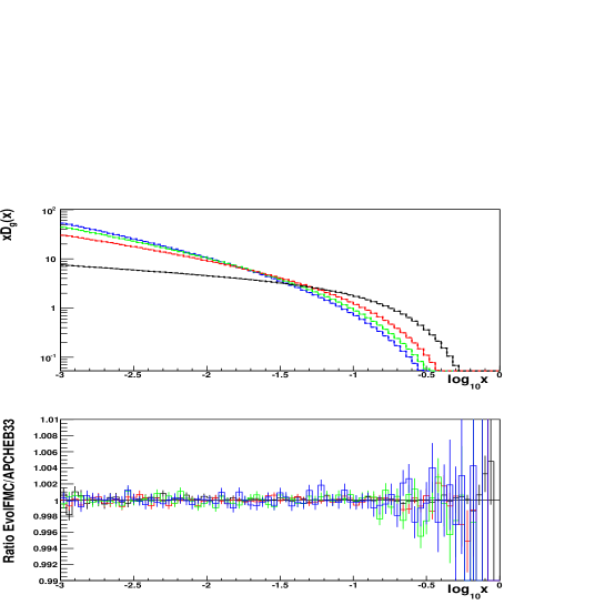
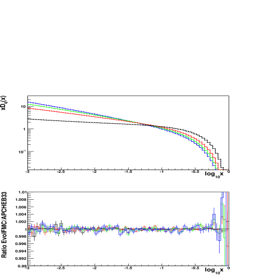
Figure 1: The upper plot shows the quark distribution $xD_{q}(x,Q_{i})$ evolved from $Q_{0}=1\,$GeV (black) to $Q_{i}=10$ (red), $100$ (green) and $1000$ (blue) GeV, obtained in the NLO approximation from EvolFMC (solid lines) and APCheb33 (dashed lines), while the lower plot shows their ratio.

Figure 2: The upper plot shows the gluon distribution $xD_{G}(x,Q_{i})$ evolved from $Q_{0}=1\,$GeV (black) to $Q_{i}=10$ (red), $100$ (green) and $1000$ (blue) GeV, obtained in the NLO approximation from EvolFMC (solid lines) and APCheb33 (dashed lines), while the lower plot shows their ratio.

In Ref. [11] we have presented the results of the comparisons between EvolFMC and QCDnum16 for the gluon and quark-singlet distributions. The agreement at the level of $\sim 0.1\%$ has been found for both the LO and NLO evolution equations. Here, in Figs. 1 and 2 we show the results of the comparisons between EvolFMC and APCheb33 for the NLO evolution. APCheb33 solves the evolution equations with the use of Chebyshev polynomials [4]. As one can see, the gluon and quark-singlet distributions from the two programs agree within $\sim 0.1\%$ (the similar agreement has been found also at the LO).

5 Summary and outlook

We have constructed the Markovian Monte Carlo algorithm for solving the QCD DGLAP evolution equations at the NLO. We have implemented this algorithm in the MC program EvolFMC (in C$++$). We have cross-checked EvolFMC with the non-MC programs QCDnum16 and APCheb33, and found the agreement at the per-mill level. MC computation for the NLO evolution is $\sim 5$ times slower than for the LO evolution. Singular behaviour of the NLO $P_{FG}$ and $P_{GF}$ splitting functions at $z\rightarrow 1$ leads to large positive weights for the $F\rightarrow G$ transitions and to negative weights for the $G\rightarrow F$ transitions in the region of $z\gtrsim 0.95$. This shows the need for additional resummation in this region. So far only massless quarks have been considered, however, adding heavy quarks can be accomplished rather easily. Also extension to the NNLO seems to be straightforward. This program can be used as a testing tool for constrained MC algorithms for the ISR, see e.g. Refs. [7, 8, 9, 10]. Last but not the least, this algorithm can form a basis for the FSR parton shower MC event generator.

References

• [1] L.N. Lipatov, Sov. J. Nucl. Phys. 20 (1975) 95;
V.N. Gribov and L.N. Lipatov, Sov. J. Nucl. Phys. 15 (1972) 438;
G. Altarelli and G. Parisi, Nucl. Phys. 126 (1977) 298;
Yu. L. Dokshitzer, Sov. Phys. JETP 46 (1977) 64.
• [2] R. Ellis, W. Stirling, and B. Webber, QCD and Collider Physics (Cambridge University Press, 1996).
• [3] M. Botje, QCDNUM16: A fast QCD evolution program, 1977, ZEUS Note 97-066, http://www.nikhef.nl/ h24/qcdcode/.
• [4] K. Golec-Biernat, APCheb33, the Fortran code to be obtained from the author, unpublished.
• [5] J. Blumlein et al., A detailed comparison of nlo qcd evolution codes, in Future Physics at HERA, edited by G. Ingelman, A. De Roeck, and R. Klanner, p. 23, 1996.
• [6] S. Jadach and M. Skrzypek, Acta Phys. Polon. B35, 745 (2004), hep-ph/0312355.
• [7] S. Jadach and M. Skrzypek, Acta Phys. Polon. B36, 2979 (2005), hep-ph/0504205.
• [8] S. Jadach and M. Skrzypek, Comput. Phys. Commun. 175, 511 (2006), hep-ph/0504263.
• [9] S. Jadach and M. Skrzypek, Acta Phys. Polon. B36, 2979 (2005), hep-ph/0504205.
• [10] S. Jadach, W. Płaczek, M. Skrzypek, P. Stephens, and Z. Wa̧s, Constrained MC for QCD evolution with rapidity ordering and minimum kT, 2007, hep-ph/0703281, Report FJPAN-IV-2007-3, CERN-PH-TH/2007-059.
• [11] K. Golec-Biernat, S. Jadach, W. Placzek, and M. Skrzypek, Acta Phys. Polon. B37, 1785 (2006), hep-ph/0603031.