Constraining Models of Neutrino Mass and Neutrino Interactions with the Planck Satellite

Abstract

In several classes of particle physics models – ranging from the classical Majoron models, to the more recent scenarios of late neutrino masses or Mass-Varying Neutrinos – one or more of the neutrinos are postulated to couple to a new light scalar field. As a result of this coupling, neutrinos in the early universe instead of streaming freely could form a self-coupled fluid, with potentially observable signatures in the Cosmic Microwave Background and the large scale structure of the universe. We re-examine the constraints on this scenario from the presently available cosmological data and investigate the sensitivity expected from the Planck satellite. In the first case, we find that the sensitivity strongly depends on which piece of data is used. The SDSS Main sample data, combined with WMAP and other data, disfavors the scenario of three coupled neutrinos at about the 3.5$\sigma$ confidence level, but also favors a high number of freely streaming neutrinos, with the best fit at 5.2. If the matter power spectrum is instead taken from the SDSS Large Red Galaxy sample, best fit point has 2.5 freely streaming neutrinos, but the scenario with three coupled neutrinos becomes allowed at $<2\sigma$. In contrast, Planck alone will exclude even a single self-coupled neutrino at the $4.2\sigma$ confidence level, and will determine the total radiation at CMB epoch to $\Delta N_{\nu}^{eff}=^{+0.5}_{-0.3}$ ($1\sigma$ errors). We investigate the robustness of this result with respect to the details of Planck’s detector. This sensitivity to neutrino free-streaming implies that Planck will be capable of probing a large region of the Mass-Varying Neutrino parameter space. Planck may also be sensitive to a scale of neutrino mass generation as high as 1 TeV.

I Introduction

Cosmology and particle physics are becoming increasingly linked, as is particularly evident in the dark sector, comprising dark matter, dark energy and dark radiation (neutrinos or other thermalized relativistic particles). Considerable work has been done to discover the nature of the new particle physics underlying the cosmological dark sector. While much remains unknown about it, the current abundance of data, combined with more precise measurements in the future, promise to give a clearer window into the dark. In this paper we consider the neutrino fraction of the dark sector. Cosmology already tells us a number of interesting facts about the neutrino sector when the universe was in its infancy. Big Bang Nucleosynthesis (BBN), for example, places significant constraint on the amount of radiation at $T\sim 1\mbox{ MeV}$, translating to an effective constraint on the total number of thermalized neutrino species, $N_{\nu}^{eff}<4.5$ Cyburt et al. (2005). The strongest upper bound on neutrino mass is also currently derived from the matter power spectrum on small scales, and the current limit is $\sum m_{\nu}<0.17\mbox{ eV}$ at 95% C.L., as given in Seljak et al. (2006).

From a particle physics perspective, there are many well-motivated models which generate beyond-the-standard-model neutrino physics, potentially giving rise to signals in the early universe. Most of these proposals could be classified into one of the following four broad categories: suggestions that neutrinos have (i) small but nonzero masses Pontecorvo (1968); Gribov and Pontecorvo (1969); (ii) interactions with electromagnetic fields (via magnetic/transition moments) Cisneros (1971); Okun et al. (1986); (iii) interactions with new heavy states Wolfenstein (1978); (iv) interactions with new light states Chikashige et al. (1981); Gelmini and Roncadelli (1981). As is well known, the first of these ideas has actually proven true, giving us the first direct discovery of physics beyond the standard model. While it is certainly possible that there are no other observable effects of new physics, it is intriguing to think that the neutrino sector could hold more surprises. The pragmatic approach is to set aside any theoretical prejudice (which has proven rather unhelpful in the past in predicting neutrino properties) and settle the issue experimentally. Should new neutrino interactions be discovered, the theoretical implications would be profound.

Testing neutrino properties in terrestrial experiments has been very challenging. It took three decades from the first indication of the “solar neutrino problem” Davis et al. (1968) to conclusively demonstrate that neutrinos are massive and oscillate. As for the other proposals on the list, progress has been even slower. In the case of non-standard neutrino interactions mediated by novel heavy particles, bounds from accelerator-based experiments Berezhiani and Rossi (2002); Davidson et al. (2003), solar Friedland et al. (2004a); Guzzo et al. (2004); Miranda et al. (2006), atmospheric Friedland et al. (2004b); Friedland and Lunardini (2005) and beam neutrino experiments Kitazawa et al. (2006); Friedland and Lunardini (2006) remain quite weak to this day. Bounds on the electromagnetic moments changed little over the last 15-20 years, with the best constraints coming from cooling of astrophysical systems such as red giants before helium flash Raffelt (1990). Finally, while certain models of neutrino coupling to light scalar fields (those involving weak doublet Aulakh and Mohapatra (1982); Santamaria and Valle (1987) or triplet Gelmini and Roncadelli (1981) fields) have been ruled out by the LEP data on the $Z$ boson width, a large class of models (involving coupling to singlet fields) remains viable (see, e.g., Berezhiani et al. (1992)).

In this paper, we show that the experimental sensitivity to nonstandard interactions mediated by a new light particle is about to be significantly improved. In this case the experimental tools are cosmological observations rather than neutrino oscillation experiments. The new interaction can manifest itself through large scattering rates of the neutrinos with themselves (and the new light fields), or through extra radiation in the early universe (through thermally populating the new light states). As we will show, while the present cosmological data yields limited constraints on the scenarios in question, the data on the Cosmic Microwave Background (CMB) anisotropies expected in the next several years from the Planck satellite mission (scheduled to launch in 2008) will lead to qualitative improvements.

There are many models which generate strong neutrino interactions. A sterile neutrino added to the standard model may have its mass generated by a scalar field in analogy with the Higgs mechanism (though the mass-generating scalar is not, by necessity, the Higgs boson since the sterile neutrino carries no standard model interactions). That scalar will mediate neutrino interactions, and the size of the coupling is often large enough to make them measurable in the CMB. Cases in point are Mass-Varying Neutrinos (MaVaNs) Fardon et al. (2004, 2006), a theory of neutrino dark energy, or a model of “late” neutrino masses Chacko et al. (2004, 2005). These theories feature neutrino-scalar interactions of a size which, as we will see, may be large enough to be measurable by the Planck satellite. We will see that Planck alone will be able to observe or rule out scenario with a single interacting and two standard neutrinos at the 4.2 $\sigma$ level.

In many models, additional scalars may also become thermally populated. It is possible to choose the parameters such that the scalars recouple after the BBN era Beacom et al. (2004); Chacko et al. (2004). Hence an independent CMB constraint becomes of great interest. Though the present constraints on $N_{\nu}^{eff}$ are not very strong in comparison to the BBN constraints, we will also find that Planck will be able to observe a single extra neutrino at approximately 2.5 $\sigma$ level.

It has been shown that in the case of interactions mediated by heavy particles cosmology does not yield effective new bounds Mangano et al. (2006). Why is the situation different when the new particles are light? The basic idea can be easily stated. Coupling neutrinos to a light scalar field can populate additional degrees of freedom in the early universe, changing the expansion rate as well as the evolution of inhomogeneities. Moreover, it can drastically increase the neutrino-neutrino interaction cross section, much more than what is possible with heavy new particles, turning the neutrinos in the early universe into a self-coupled fluid. The neutrino density perturbations would evolve differently from the standard case – coupled neutrinos would undergo acoustic oscillations rather than stream freely in the CMB epoch ($T\sim 1-10$ eV) – and affect the baryon-photon fluid and dark matter through their gravity during the epoch of radiation domination.

Our cosmological analysis is done in a rather model-independent way. For most of the parameter space, one can simply assume that in the CMB epoch there is a certain number of free streaming relativistic species, $N_{FS}$ (the standard neutrinos fall into this category), and a certain number of relativistic species forming a self-coupled fluid, $N_{coupled}$. This approach is certainly not new Chacko et al. (2004); Bell et al. (2006). We will denote the total number of effective neutrinos (which includes any thermalized radiation, whether free-streaming or coupled) as $N_{\nu}^{eff}$. The results then have a broader applicability. For example, if one sets $N_{coupled}=0$, one obtains a bound on the total number of the standard neutrinos. The constraints on the latter from the current data, as well as forecasts for Planck, have been investigated in numerous recent studies Bell et al. (2006); Seljak et al. (2006); Cirelli and Strumia (2006); Hannestad and Raffelt (2006), Bowen et al. (2002); Bashinsky and Seljak (2004); Perotto et al. (2006), with somewhat differing results. We will weigh in on this controversy.

The cosmology of neutrinos coupled to a light scalar is a very old topic. Over the years, different aspects of it were discussed in Georgi et al. (1981); Kolb and Turner (1985); Raffelt and Silk (1987); Atrio-Barandela and Davidson (1997), Chacko et al. (2004); Beacom et al. (2004). Four modern data analyses are those by Hannestad Hannestad (2005), by Trotta and Melchiorri Trotta and Melchiorri (2005), by Bell, Pierpaoli, and Sigurdson Bell et al. (2006), and by Cirelli and Strumia Cirelli and Strumia (2006). These papers only analyze the existing data and do not forecast the reach of Planck. Moreover, once again, the results these papers find with the available data differ. We will reexamine this situation using up-to-date cosmological data.

In the next Section we examine in more detail the types of neutrino models which generate strong neutrino interactions or extra relativistic degrees of freedom. We then turn to the CMB phenomenology of constraining these models. We carry out an analysis using all the current cosmological data, and determine the precision with which Planck will be able to constrain neutrino interactions. We then apply these constraints to Majorana neutrino interactions and consider the implications for theories of neutrino dark energy (MaVaNs). The details of our analysis are contained in Sects. III-V; the Reader with interests in cosmology may wish to focus on these Sections. Conversely, the Reader who is interested only in the implications for neutrino models can proceed directly from Sect. II to Sect. VI.

II Models of Neutrino-Scalar Interactions

As mentioned in the Introduction, the possibility of coupling the neutrinos to a novel light scalar field has been entertained in the literature since the early 1980’s. In this Section, we will briefly review some of the cosmologically relevant features of the many models that were constructed. For more details, the Reader should consult, e.g., Chikashige et al. (1980, 1981); Gelmini and Roncadelli (1981); Georgi et al. (1981); Aulakh and Mohapatra (1982); Santamaria and Valle (1987); Berezhiani et al. (1992) and many other papers dedicated to the subject.

From the point of view of cosmological constraints based on the CMB, we are interested in the physics at 1 eV energies. At these low energies the relevant properties of the full models are captured by effective low-energy Lagrangian terms. We may thus try to learn about some of the common features of the models by building this interaction “bottom-up”.

The starting step may be to seek an interaction of the Yukawa type, $g\phi\nu\nu$. To have the correct gauge structure, the neutrino field must be promoted to the lepton doublet. At the level of dimension 4 operators one can then write $L^{c}\bm{\tau}\bm{\cdot}\bm{\phi}L$. This means the new scalar field $\bm{\phi}$ is a triplet of $SU(2)$ and couples to the $Z$ boson. If one further writes a symmetry breaking potential for $\bm{\phi}$ (to obtain a massless Goldstone boson – a Majoron), one obtains the classical model of Gelmini and Roncadelli Gelmini and Roncadelli (1981). This model has been ruled out by the LEP measurements of the $Z$ boson width: the triplet Majoron would contribute an equivalent of two extra neutrino species to the width. This argument extends to other models in which the new light scalar is not a singlet of $SU(2)$; for instance, the Higgs doublets Aulakh and Mohapatra (1982); Santamaria and Valle (1987) would contribute a half of an extra neutrino species to the $Z$ width. As a consequence, we must assume that the light scalar field is a Standard Model singlet.

The simplest renormalizable model that generates an effective low-energy neutrino-scalar coupling involves adding a right-handed sterile neutrino $N$ to the theory and coupling a scalar $\phi$ to it. To this end, consider the standard see-saw mechanism. The mixing of $N$ with the Standard Model neutrinos only enters through a Dirac neutrino mass term, so that the neutrino Lagrangian contains

$${\delta\cal L}=yLHN+m_{N}NN.$$ (1)

The first term is of the same form as the lepton Dirac masses in the Standard Model, while the second one is a Majorana mass term for the right-handed (sterile) neutrino. When the sterile neutrino is integrated out, assuming $m_{N}\gg m_{D}\equiv yv$, only a light Majorana neutrino remains, with mass $y^{2}v^{2}/m_{N}$.

We may now promote the sterile neutrino mass, $m_{N}$, to a dynamical (complex) field $\phi$, in analogy to the Standard Model Higgs mechanism, where the Dirac mass is generated by the dynamical Higgs :

$${\delta\cal L}=yLHN+\lambda\phi NN.$$ (2)

When $\phi$ develops a VEV, $\left<\phi\right>={f}$, the sterile neutrino gets a mass $m_{N}=\lambda{f}$ and can be integrated out of the theory. The light Goldstone mode $G$ ($\phi\equiv({f}+\rho)e^{-iG/{f}}$) is coupled to the light neutrinos via an effective interaction of the form

$$\frac{y^{2}}{\lambda{f}}e^{iG/{f}}(L\left<H\right>)(L\left<H\right>).$$ (3)

Clearly, at the energies of $O(1)$ eV the Higgs field in Eq. (3) has no excitations, only the vacuum expectation values (VEVs), $\left<H\right>=v$.

An alternative form of the interaction can be obtained by absorbing $e^{iG/f}$ into the phase of $L$. The interaction then appears from the kinetic term for $L$,

$$\frac{i}{f}\partial_{\mu}G\bar{L}\bar{\sigma}^{\mu}L+h.c.$$ (4)

This form makes manifest the derivative nature of the coupling of $G$.

We note that while the construction reviewed here is the simplest, it is certainly not unique. In general, the scalar field need not couple to only the sterile neutrino and could be coupled via both the Dirac and Majorana terms in Eq. (1), e.g., by promoting $y\rightarrow\phi/\Lambda$, $m_{N}\rightarrow\Phi^{2}/\Lambda$ Chacko et al. (2005).

Expanding Eq. (3) to the first order in $G$, we find a Majorana mass for $L$, $m_{\nu}=y^{2}v^{2}/(\lambda{f})$ (where $v=\langle H\rangle$) and an effective Yukawa (pseudoscalar) interaction of $G$ with $L$, with the coupling strength

$$g=\frac{y^{2}v^{2}}{\lambda{f}^{2}}=\frac{\lambda m_{D}^{2}}{m_{N}^{2}}=\frac{m_{\nu}}{{f}}.$$ (5)

The second equality has a very simple physical interpretation: $m_{D}^{2}/m_{N}^{2}$ gives the amount of admixture of the sterile neutrino into the light mass eigenstate and $\lambda$ is the coupling of $g$ to the sterile component.

In order to generate a sizable coupling $g$ between the neutrino and scalar, there must not be too large a hierarchy between $m_{\nu}$ and the scale of symmetry breaking $f$. If the sterile neutrino mass is at GUT scale, the coupling of $G$ is of the size $g\sim 10^{-25}$, assuming $m_{\nu}\sim 0.1\mbox{ eV}$ and $\lambda\sim 1$, which is too small to give rise to significant effects during the CMB epoch. On the other hand, if the scale of new physics, $\Lambda$, is TeV scale, couplings of the size $g\sim 10^{-13}$ may be generated. Though this is a very small coupling, it is large enough to result in observable effects through decay-inverse decay of the neutrino to scalars, which tightly couples the scalars and neutrinos, removing neutrino free-streaming. We return in detail to the constraints on the coupling $g$ in Sect. VI.

There are many theories where a coupling $g>10^{-13}$ is generated. Theories of neutrino dark energy introduce interactions in the effective theory of the form Eq. 2, often with a sizable coupling $g$. In the models of dark energy originally discussed in Frieman et al. (1992) and revived in Hill et al. (2006) as neutrino dark energy, the scalar generating the dark energy is a pNGB. If the scale of the symmetry breaking $f$ of the scalar U(1) symmetry is sufficiently low (TeV scale or lower), a cosmologically interesting coupling between the scalar and neutrino may be generated. Since the scalar is a pNGB in these models, it is protected from large radiative corrections, and hence remains light–an advantage in any theory of dark energy. In a similar model of Barbieri et al. (2005), $f\sim M_{pl}$, but $m_{N}$ and $m_{D}$ are small, through extremely small Yukawa couplings $y$ and $\lambda$ to the neutrino mass generating fields $H$ and $\phi$. Since $\lambda$ is very small, $g$ is also very small and there are no observable consequences in the CMB through the neutrino-scalar coupling. Because the sterile neutrino is light, however, and the mixing between the active and sterile neutrino is substantial, the sterile neutrino may become thermalized, and there may be signals in the CMB through increased $N_{FS}$.

Another theory of dark energy may also generate interesting signals in the CMB. In contrast to these models where the scalar field is typically associated with a broken symmetry at a comparatively high scale $f$, MaVaNs, as introduced in Fardon et al. (2004), place the entire sector around a meV–this scale is chosen according to the measured neutrino mass splittings and the dark energy scale $\delta m_{\nu}^{2}\sim 10^{-1}\mbox{ eV}$, $\Lambda_{DE}\sim 10^{-2.5}\mbox{ eV}$. As a consequence, all mass scales in the model, including the Dirac mass and the scalar mass, lie in the sub-eV range, and the coupling $\lambda$ is typically not too small; the small hierarchy between the Dirac and sterile neutrinos implies a sizable coupling $g$ in many cases.

There are many other instances where the hierarchy between the Dirac neutrino and sterile neutrino is much smaller due to the introduction of lighter sterile neutrinos. Much lighter sterile neutrinos have been considered in a wide variety of contexts, most notably perhaps in connection with the LSND measurement, where the presence of a sterile neutrino with mass around $1\mbox{ eV}$ has been invoked to explain the appearance of muon neutrinos Gonzalez-Garcia and Nir (2003). Other models feature a keV mass sterile neutrino as the dark matter Dodelson and Widrow (1994); Abazajian et al. (2001); Shi and Fuller (1999), sometimes with accompanying keV mass scalars Kusenko (2006), and weak scale neutrinos associated with SO(10) GUTS, where the addition of the neutrino is necessary for anomaly cancellation Raby (2002). Various low energy see-saws have also been considered, as in Chacko et al. (2004), where the scale $f$ is in the 50 MeV to 500 GeV range.

We have seen that there is a broad class of models which generate exotic neutrino-scalar interactions. The addition of these interactions, depending on the choices of $\lambda$, $m_{D}$ and $m_{N}$, may be good candidates for observation in the cosmic microwave background. First, additional scalars may become thermalized and increase the effective number of neutrino species. Second, these scalars mediate additional neutrino interactions, through scalar mediated neutrino scattering, which could remove neutrino free-streaming at CMB temperatures. We now turn our attention to studying the impact of non-standard behavior in the dark radiation sector on CMB anisotropies.

III Tightly coupled neutrinos: modified evolution equations.

We summarize the relevant physical effects of dark radiation (i.e. neutrinos) on the CMB. The energy density in relativistic neutrinos is a fraction $\simeq N_{\nu}^{eff}/(N_{\nu}^{eff}+4.4)$ of the total radiation (freely-streaming and coupled neutrinos plus photons). Thus during the radiation epoch the neutrino gravity is important. One needs to consider both the effects of the neutrino background density and that of the neutrino density perturbations. $N_{\nu}^{eff}$ dictates the expansion rate of the universe and, together with matter density $\Omega_{m}h^{2}$, controls the redshift of matter-radiation equality, $z_{eq}$. The latter effect is more subtle. Assuming adiabatic initial conditions, the neutrino and photon inhomogeneities are of comparable size to begin, so the presence of neutrinos modifies the evolution of the photon perturbations. When a perturbation of a given size enters the horizon, the gravity of the neutrino perturbation is comparable to the gravity of the photon perturbation. The subsequent evolution of the two, however, are different. The photon-baryon plasma oscillates like a compressible fluid; the standard neutrinos, on the other hand, stream freely, quickly erasing their density fluctuations. Gravitational coupling between the two means that the evolution of fluctuations in the photons could be affected by neutrino free-streaming. In fact, Stewart Stewart (1972) noted back in 1972 that if this effect were large, it would jeopardize structure formation.

Shortly thereafter, Peebles Peebles (1973) numerically solved the problem of the coupled evolution of the neutrino and photon perturbations. He showed that the neutrino inhomogeneities in the standard case do indeed decay shortly after entering the horizon; in the process, they damp photon inhomogeneities, although at a significantly smaller level ($\sim$12%) than anticipated by Stewart. Much more recently, the problem was addressed by more accurate numerical computations and analytically Hu and Sugiyama (1996); Bashinsky and Seljak (2004) and for the CMB power spectrum the amount of suppression (relative to the case where all the radiation is strongly coupled) was found to be

$$\delta C_{\ell}/C_{\ell}\approx-0.53\,\rho_{FS}/\rho_{rad},$$ (6)

where $\rho_{FS}$ is the energy density in freely streaming radiation and $\rho_{rad}$ is the total radiation density (free-streaming plus strongly coupled, including photons).

Coupling the oscillating photons to the damped neutrinos through the gravitational potential also changes the phase of the photon oscillations, due to a change in the speed at which information propagates in the fluid from the presence of freely streaming neutrinos, compared to the hypothetical case of no free-streaming neutrinos. This effect was clearly established in Bashinsky and Seljak (2004). The resulting shift of the CMB peaks is

$$\delta\ell\approx-57\,\rho_{FS}/\rho_{rad}.$$ (7)

Remarkably, both the amplitude suppression and phase shift are clearly present in the Peebles’ solution . These effects are at the core of the physics behind the sensitivity of CMB to neutrino free-streaming. The amount of damping and the phase shift change if either additional freely streaming relativistic (“neutrino-like”) species are added or the neutrinos become self-coupled. In the latter case, both effects are removed: the neutrino fluid oscillates similarly to the photon fluid (without baryon loading).

Notice that the effect is not uniform for all CMB multipoles. The above argument was made for modes entering the horizon in the radiation era. For modes entering the horizon in the matter era, the neutrino perturbations have no effect. Thus, the damping is operational only on small scales, $l\gtrsim 200$.

In our analysis, we consider interacting neutrinos in the tightly coupled limit. By this we mean that the neutrinos can be approximated by a fluid for the entire range of relevant scales, including the scales corresponding to the CMB multipoles of $l\sim 2000$ and those measured by the large scale structure (LSS) surveys SDSS and 2dF. The neutrino analogue of the Silk damping scale is thus assumed to be well below $\sim O(10)$ comoving Mpc. The implications of this assumption are further discussed in Sect. VI.

With the above assumptions, the Boltzmann equations for the coupled neutrinos are very simple, as discussed in Hu et al. (1995): the standard multipole expansion for the neutrino perturbations (see Ma and Bertschinger (1995)) is truncated at the level of density and velocity perturbations. The quadrupole (shear) and higher order moments of the perturbations are set to zero. The analogues of Eqs. (49) or (50) in Ma and Bertschinger (1995) are:

• Synchronous gauge

$$\dot{\delta}_{\nu} = -\frac{4}{3}\theta_{\nu}-\frac{2}{3}\dot{h},$$

$$\dot{\theta}_{\nu} = \frac{1}{4}k^{2}\delta_{\nu},$$

$$\sigma_{\nu} = 0.$$ (8)

• Conformal Newtonian gauge

$$\dot{\delta}_{\nu} = -\frac{4}{3}\theta_{\nu}+4\dot{\phi},$$

$$\dot{\theta}_{\nu} = \frac{1}{4}k^{2}\delta_{\nu}+k^{2}\psi,$$

$$\sigma_{\nu} = 0.$$ (9)

Here all the conventions are those of Ma and Bertschinger (1995). The quantity $\delta_{\nu}\equiv\delta\rho_{\nu}/\rho_{\nu}$ is the neutrino density perturbation; $\theta_{\nu}\equiv ik^{j}\delta T^{0}_{\phantom{0}j}/(\bar{\rho}+\bar{P})$, with the “$\nu$” index assumed on the right hand side, is the neutrino velocity perturbation; $\sigma$ is the shear (see Eq. (22) of Ma and Bertschinger (1995)). The quantity $h$ is one of the two scalar perturbations in the synchronous gauge (the one corresponding to the trace of the scalar metric perturbation). $\phi$ and $\psi$ are the scalar metric perturbations in the Conformal Newtonian gauge. They coincide, up to a sign, with the gauge invariant Bardeen variables Bardeen (1980).

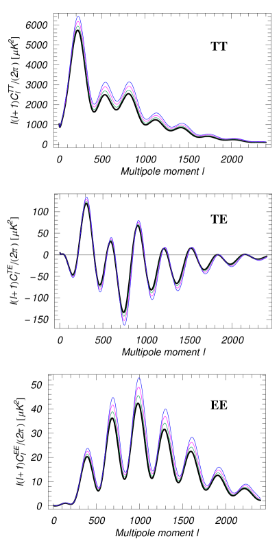
Figure 1: Effect of neutrino free-streaming on the CMB multipole spectrum. The thickest curve is the spectrum with the best fit parameters from WMAP3; the other curves (from bottom to top) correspond to 1, 2, and 3 strongly coupled neutrinos (keeping the total number of neutrinos fixed at 3).

The same method of truncating the multipole expansion is utilized in the earlier analyses. Our equations agree with those of Hannestad (2005); Bell et al. (2006) (which are stated in the synchronous gauge) and those of Cirelli and Strumia (2006) (which are stated in the Conformal Newtonian gauge). We note that the CAMB Lewis et al. (2000) code we use (also CMBFast Seljak and Zaldarriaga (1996)) employs the synchronous gauge. A slightly more general parameterization in terms of the “viscosity parameter”, $c_{vis}^{2}$ Hu (1998) is followed in Trotta and Melchiorri (2005).

The effect of making the neutrinos coupled, for fixed cosmological parameters, is illustrated in Fig. 1. The thick curve refers to the standard case of three freely streaming neutrinos, while the other curves illustrate the effect of coupling 1, 2, and 3 neutrinos (in order of deviation from the thick curve). The changes of the temperature (TT), polarization (EE), and the cross correlation between them (TE) are shown. The Figure clearly exhibits both the amplitude suppression and the phase shift effects at $l\gtrsim 200$.

The difference in the anisotropies on scales $l\gtrsim 200$ is quite large (on average about 25-30% for three coupled neutrinos), well outside the errors of the current WMAP data. However, this does not mean than the coupled neutrino scenario is already excluded. Indeed, it must be kept in mind that there are many cosmological (“nuisance”) parameters that can be adjusted, such as the baryon, dark matter and dark energy densities, the spectrum of primordial fluctuations, and others. By adjusting these parameters, it may be possible to undo most of the effect of the neutrino self-coupling.

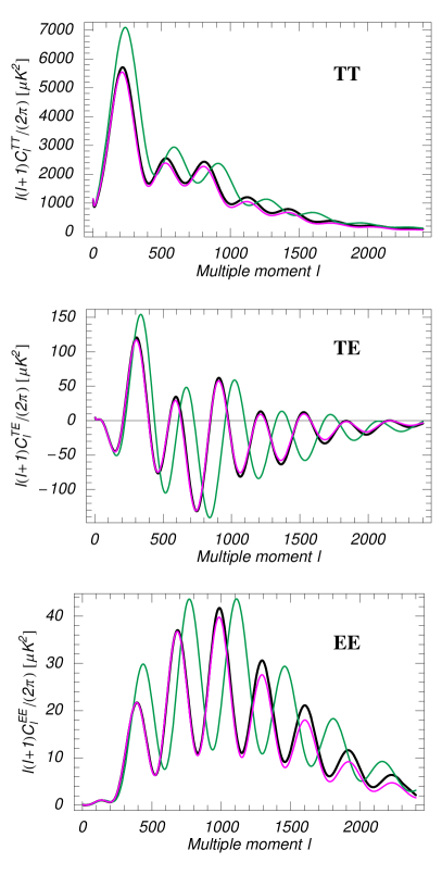
Figure 2: Effect of extra neutrinos on the CMB multipole spectrum. The central black curve is the spectrum with the best fit parameters from WMAP3, the top green curve the spectrum with 7 freely streaming neutrinos, and the lowermost magenta curve results when the total number of freely streaming neutrinos is 7, but $z_{eq}$ is kept fixed by varying $h^{2}$.

This issue of “degeneracies” between different parameters is of course well known in cosmology. A simple illustration of it is given in Fig. 2 where we show changing the CMB power spectra as one changes the total number of freely streaming neutrinos. While simply changing $N_{FS}$ to 7 produces a large shift in the position of the peaks (because of the faster expansion in the radiation era as discussed above), the effect can be compensated by changing other parameters such that the redshift of equality is preserved Bowen et al. (2002). $1+z_{eq}=4.05\times 10^{4}\Omega_{m}h^{2}/(1+0.6905N_{\nu}^{eff}/3.04)$ is fixed while varying $N_{\nu}^{eff}$ by scaling $h^{2}$ to compensate for the increase in $N_{\nu}^{eff}$, while also fixing the physical baryon density $\Omega_{b}h^{2}$ and $\Omega_{m}$. Indeed, the physical quantities that are measured in CMB are dimensionless quantities (angles on the sky), hence they depend on the ratios of the physical densities, etc. See, e.g., Bashinsky (2004) for further discussion.

Not all effects follow this simple argument. For example, the Silk damping does not, as it involves a physical dimensionful constant, the Thompson cross section. The faster expansion of the universe with more neutrinos implies more Silk damping in the high multipoles of the CMB . This can be partially compensated by adjusting the Helium fraction, as discussed in Bashinsky and Seljak (2004). It should be kept in mind that this mechanism is limited by a variety of astrophysical considerations. We will return to this topic in Sect. V.2.

The real challenge is to establish the size of the residual differences of the CMB predictions in the two scenarios, after appropriately adjusting the “nuisance” parameters, in comparison with the resolution of the experiments. These residual differences turn out to be much smaller than the differences seen in Fig. 1. This fact renders difficult writing down a simple estimate for the predicted sensitivity of the present and future experiments using order-of-magnitude arguments and necessitates a detailed scan of the multidimensional parameter space.

In Sect. V.2 we show how well the effects of amplitude suppression (6) and phase shift (7) can be compensated by adjusting the cosmological parameters and how big the residual differences are. We will also see which CMB multipoles are essential for testing the neutrino sector and how robust our predictions for Planck are. A complete analysis of this type has not been done before.

We now present the results of our numerical studies.

IV Numerical results

IV.1 Sensitivity of the current data

IV.1.1 Literature overview

We begin by summarizing the bounds on the numbers of freely streaming and self-coupled relativistic species derived in the literature. In the case of extra relativistic species, a number of studies have been undertaken in the last several years. Crotty, Lesgourgues, and Pastor found the effective number of neutrinos to lie in the interval $[1.4,6.8]$ at $95\%$ confidence level (C.L.), by combining WMAP year one data Bennett et al. (2003) with the LSS data from 2dF Hawkins et al. (2003) and a prior on the Hubble constant. Similar results were found by Pierpaoli Pierpaoli (2003) and Hannestad Hannestad (2003). Bell, Pierpaoli, and Sigurdson Bell et al. (2006) have shown that WMAP year one data Bennett et al. (2003), Lyman-$\alpha$ forest Viel et al. (2004), and Sloan Digital Sky Survey (SDSS) data Tegmark et al. (2004) taken together constrain the effective number of neutrinos to be $4.9_{-2.3}^{+1.9}$ at $95\%$ C.L. Seljak, Slosar and McDonald Seljak et al. (2006) have also computed this number with more recent data – including the WMAP three year data (WMAP3) Hinshaw et al. (2006); Page et al. (2006), Lyman-$\alpha$ forest data McDonald et al. (2005), SDSS measurements of the baryon acoustic oscillations Eisenstein et al. (2005) (see Seljak et al. (2006) for a complete list). They find a similar result, $N_{FS}=5.3^{+2.1}_{-1.7}$ at 95% C.L. The WMAP team finds year-3 data combined with large-scale structure and supernovae prefer $3.3\pm 1.7$ neutrinos Spergel et al. (2006). Cirelli and Strumia Cirelli and Strumia (2006) find $N_{FS}=5\pm 2$ ($2\sigma$ errors). In contrast, Hannestad and Raffelt Hannestad and Raffelt (2006), constraining neutrino mass and relativistic energy density together, determine $2.7<N_{FS}<4.6$ at 95% C.L. using WMAP3 and large-scale structure data from 2dF and SDSS.

In the case of self-interacting neutrinos, all fits are consistent with no interactions, but with (very) different confidence levels. Hannestad Hannestad (2005) concludes that in the model with three interacting neutrinos “it is impossible to simultaneously fit CMB and LSS data”. From his Fig. 8 we read off a 3$\sigma$ exclusion using only WMAP1 and 6$\sigma$ exclusion when this data is combined with the SDSS LSS data and the HST Hubble constant measurement (in the limit of zero neutrino mass). In contrast, Trotta and Melchiorri Trotta and Melchiorri (2005) find that the interacting neutrino scenario is disfavored at only 2.4$\sigma$. Similarly, Bell, Pierpaoli, and Sigurdson find $N_{coupled}<3.0$ at 95% C.L. Cirelli and Strumia find the number of additional interacting neutrinos constrained to be less than $1.3$ at $1\sigma$ with more recent data (including WMAP3).

In short, there is quite a bit of variation between the published results. Some of this variation could be attributed to different data used in the calculations (for example, WMAP 1-year vs. WMAP 3-year data releases, whether Lyman-$\alpha$ was included in the analysis or not, etc), but some clearly must be due to the differences in the analyses themselves. We therefore consider it well-motivated to repeat the calculations, using the most recent data available to us. In Sect. IV.1.2 we consider the sensitivity of WMAP3 alone, while in Sects. IV.1.3 and IV.1.4 we add other cosmological data.

As far as forecasting for Planck, published results on $N_{FS}$ likewise differ. In addition, no analysis on $N_{coupled}$ has been performed. Ref. Bowen et al. (2002) finds that Planck will be able to constrain the total number of freely streaming neutrino species to $\Delta N_{FS}=0.24$ (1$\sigma$ error) using temperature information only and a sky coverage $f_{\rm sky}=0.5$. In contrast, Ref. Bashinsky and Seljak (2004) finds using Planck temperature information only $\Delta N_{FS}=0.6$ even with a more optimistic sky coverage $f_{\rm sky}=0.8$. Both studies employ the same technique (the Fisher matrix analysis). Finally, Ref. Perotto et al. (2006) investigated the bounds on $N_{FS}$ using both the Fisher analysis and Markov Chain Monte Carlo (MCMC). The results are quite intriguing: while the Fisher analysis yields $\Delta N_{FS}=0.26(0.27)$ with (without) lensing, the MCMC method yields very different results depending upon whether lensing is assumed – with lensing the result is consistent with the Fisher analysis, while without lensing $\Delta N_{FS}=0.46$. The forecast for Planck’s sensitivity to the number of self-coupled neutrinos to the best of our knowledge has not been done. We perform a combined analysis of Planck’s sensitivity to freely streaming and self-coupled neutrino species in Sect. IV.2.1. We also investigate, in Sect. IV.2.2, a potential impact of combining Planck with other cosmological data.

IV.1.2 WMAP3 alone

$(N_{FS},N_{coupled})$	$\delta\chi^{2}$	C.L.	$\Omega_{b}h^{2}$	$\Omega_{c}h^{2}$	$\theta$	$\tau$	$n_{s}$	$\log[10^{10}A_{s}]$	$\Omega_{\Lambda}$	Age/GYr	$\Omega_{m}$	$z_{re}$	$H_{0}$
$(3,0)$	–	–	$0.02216$	$0.10519$	$1.0394$	$0.089$	$0.953$	$3.02$	$0.76$	13.75	0.24	11.3	72.8
$(2,1)$	0.2	$0.1\sigma$	$0.02249$	$0.10478$	$1.0423$	$0.078$	$0.927$	$2.93$	$0.77$	13.66	0.23	10.2	73.8
$(1,2)$	0.4	$0.2\sigma$	$0.02323$	$0.10367$	$1.0472$	$0.080$	$0.907$	$2.86$	$0.78$	13.43	0.22	10.1	76.5
$(0,3)$	1.4	$0.7\sigma$	$0.02436$	$0.09828$	$1.0542$	$0.095$	$0.897$	$2.80$	$0.82$	13.06	0.18	11.0	83.0
$(1,0)$	0.6	$0.3\sigma$	$0.02201$	$0.07183$	$1.0521$	$0.091$	$0.914$	$2.88$	$0.77$	15.82	0.23	10.0	64.1
$(5,0)$	0.6	$0.3\sigma$	$0.02187$	$0.13921$	$1.0312$	$0.088$	$0.968$	$3.08$	$0.74$	12.40	0.26	12.2	79.3

Table 1: The best fit values of $-log(likelihood)$ (second column) and the corresponding shift of the best fit parameters as a function of the number of coupled neutrinos. The last five columns list derived parameters. The initial spectrum is defined with a pivot point $k_{piv}=0.05$ Mpc^-1. The fit is to the WMAP3 dataset only.

As a first calculation, we investigate how sensitive WMAP is by itself to neutrino self-coupling. We do this by fitting WMAP3 Hinshaw et al. (2006); Page et al. (2006), varying a set of cosmological parameters (to be specified shortly) under four different assumptions: (i) three standard free-streaming neutrinos; (ii) one neutrino coupled, two free-streaming; (iii) two neutrinos coupled, one free-streaming; (iv) all three neutrinos coupled. We then compare the goodness of fit at the corresponding best-fit points. We also explore the sensitivity of WMAP to the total number of (standard) neutrinos, in a similar way. For this, we consider two more scenarios: one with the total neutrino number equal to five and another with a single neutrino flavor.

The fitting is done using the MCMC code COSMOMC Lewis and Bridle (2002), with the CAMB code Lewis et al. (2000) modified by us to include both freely streaming and tightly self-coupled neutrinos. The MCMC method is by now a standard tool in cosmology, used for both data analysis and forecasting. It is employed by the WMAP Spergel et al. (2003, 2006) and Planck Planck Collaboration teams, as well as many other groups (in particular, among the papers reviewed in Sect. IV.1.1, Trotta and Melchiorri (2005); Bell et al. (2006); Seljak et al. (2006); Perotto et al. (2006) use MCMC). With the MCMC method, the likelihood function is mapped out in a multidimensional region of parameters around its maximum. As a result, one gets the location of the best-fit point, with the corresponding likelihood characterizing the goodness of fit, as well as the allowed ranges of the parameters. One need not make a priori assumptions on the functional form of the likelihood function, although choosing the parameterization in such a way that the posterior distributions are approximately Gaussian and there are no strong correlations saves computer time Lewis and Bridle (2002) .

In this Subsection, we choose the following six cosmological parameters: the physical densities of baryons, $\Omega_{b}h^{2}$, and dark matter, $\Omega_{c}h^{2}$, the ratio of the approximate sound horizon to the angular diameter distance $\theta$, the optical depth to the last scattering surface $\tau$, and the primordial spectrum of the scalar curvature perturbations, characterized by the spectral index $n_{s}$ and the power $A_{s}$ on a preset (“pivot”) scale (taken in this calculation to be $k_{piv}=0.05$ Mpc^-1). We assume that the Universe is flat, there is no running of the spectral index, the Helium fraction is fixed at $Y_{\rm He}=0.24$ and the dark energy is a cosmological constant ($w=-1$). As we will see, in the case of WMAP3, the six parameters we vary contain the necessary degeneracies with the neutrino coupling.

The results are tabulated in Table 1. The first row corresponds to the standard scenario, $N_{FS}=3,N_{coupled}=0$. The next three rows correspond to coupling one, two, or three of the neutrino species, while keeping the total number of neutrinos at three. Finally, in the last two rows, we vary the total number of neutrino species, assuming they are all freely streaming.

The second column shows the difference between the $\chi^{2}$ of the best fit in a given scenario and the corresponding quantity in the standard scenario (first row). The third column shows the corresponding confidence level (C.L.) . The next six columns in the Table show the values of the best-fit parameters for each scenario. The last five columns show the values of derived parameters: the cosmological constant $\Omega_{\Lambda}$, the age of the Universe, the matter fraction $\Omega_{m}$, the red-shift of ionization $z_{re}$ and finally the Hubble constant, $H_{0}$. To compensate for the effect of neutrino coupling, $H_{0}$ increases, while $\Omega_{m}$ and the spectral index decrease. To compensate for additional neutrino species, all three quantities increase. In the latter case, it is easy to check that the best-fit parameters shift in such a way that the redshift of matter-radiation equality, $z_{eq}$, is preserved, as discussed in Sect. III. $A_{s}$ also increases with $N_{FS}$ to compensate for the reduction of perturbations on all scales.

From the second column, we see that the effects of the neutrino coupling as well as the variation of the total number of neutrinos are nearly perfectly compensated. The quality of the fits is virtually the same in each of the six cases. Therefore, WMAP by itself cannot distinguish between these scenarios. This conclusion is consistent with the findings of the analysis by the WMAP collaboration, which considers the sensitivity of the experiment to the number of freely streaming neutrino species Spergel et al. (2006). It differs from the findings of Hannestad (2005) where a 3$\sigma$ exclusion of the ($N_{FS}=0,N_{coupled}=3$) scenario was claimed. Clearly, our conclusion relies on the ability of the code to find the set of parameters that give the most complete compensation of the effects of modifying the neutrino sector. We see that the MCMC method accomplishes this task well.

IV.1.3 WMAP3 plus large scale structure (2dF, SDSS), HST, SN Ia.

$(N_{FS},N_{coupled})$	$\delta\chi^{2}$	C.L.	$\Omega_{b}h^{2}$	$\Omega_{c}h^{2}$	$\theta$	$\tau$	$Y_{\rm He}$	$n_{s}$	$n_{\rm run}$	$\log[10^{10}A_{s}]$	$\Omega_{\Lambda}$	Age/GYr	$\Omega_{m}$	$z_{re}$	$H_{0}$	$\sigma_{8}$
$(3,0)$	–	–	$0.02259$	$0.11083$	$1.0418$	$0.073$	0.244	$0.985$	0.018	$3.03$	$0.74$	13.70	0.26	9.9	71.4	0.791
$(2,1)$	4.0	$1.5\sigma$	$0.02340$	$0.11703$	$1.0478$	$0.079$	0.236	$0.956$	0.062	$3.00$	$0.73$	13.47	0.27	10.3	71.8	0.793
$(1,2)$	8.8	$2.5\sigma$	$0.02390$	$0.11993$	$1.0506$	$0.074$	0.242	$0.926$	0.008	$2.93$	$0.72$	13.36	0.28	9.8	72.0	0.770
$(0,3)$	15.6	$3.5\sigma$	$0.02406$	$0.12599$	$1.0563$	$0.074$	0.242	$0.888$	-0.017	$2.89$	$0.71$	13.18	0.29	9.9	72.5	0.776
$(1,0)$	12.3	$3.1\sigma$	$0.02296$	$0.08411$	$1.0586$	$0.083$	0.242	$0.958$	0.015	$2.98$	$0.71$	15.59	0.29	9.8	61.2	0.735
$(5,0)$	-0.3	–	$0.02210$	$0.13999$	$1.0315$	$0.090$	0.241	$0.986$	0.006	$3.10$	$0.74$	12.37	0.26	12.4	79.4	0.850

Table 2: The same as Table 1, but including WMAP3, SDSS Main and LRG data samples, 2dF, HST, and SN Ia datasets. The last column is the derived best fit value of $\sigma_{8}$.

Figure 3: The shift of the best-fit parameters as a result of neutrino coupling. The dashed-dotted curves correspond to the scenario of coupled neutrinos, while the solid ones refer to the standard (free streaming) neutrinos. In both cases, the fits are to the datasets from WMAP3, SDSS, 2dF, HST, and SN Ia.

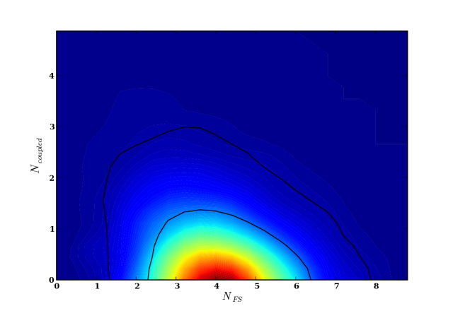
Figure 4: The combined reach of all available data (excluding Lyman-$\alpha$) on the number of free-streaming neutrinos, $N_{FS}$, and the number of coupled neutrinos, $N_{coupled}$: WMAP3 + SDSS (LRG) + SDSS (Main) + 2dF + HST + SNIa. The solid contours indicate 1 and 2$\sigma$ C.L.

We now explore if the addition of the other presently available cosmological data can lift the degeneracy of WMAP3. In this analysis, we include the data on the large scale structure (LSS) from the 2dF Cole et al. (2005) and the SDSS survey – both the Main Tegmark et al. (2004) and the recently released Large Red Galaxy (LRG) Tegmark et al. (2006) data samples. We also use the Type Ia supernova data from the SNLS collaboration Astier et al. (2006), as well as the Hubble constant measurements from the Hubble Space Telescope (HST) Freedman et al. (2001), in the form of a Gaussian prior $h=0.72\pm 0.8$.

We vary eight parameters, six as described in the previous Subsection, plus two more, the helium fraction, $Y_{\rm He}$ and the running of the spectral index, $n_{s}$. These two parameters are added in anticipation of the analysis for Planck, where their roles are important. With the present day data, as we will see, they do not make much of a difference. For the helium fraction, we use a gaussian prior $Y_{\rm He}=0.24\pm 0.009$ motivated by observational bounds Olive and Skillman (2004). We also impose a rather generous hard prior, $0.15<Y_{\rm He}<0.3$. The values greater than 0.3 would be problematic for the solar model (since the input value into the solar model cannot be less than the primordial value) Ciacio et al. (1997); Bahcall et al. (2001).

We begin by performing a combined fit to all the data. Results for several specific scenarios are shown in Table 2. We find that the degeneracies of the WMAP3-only analysis are broken by the additional data. In particular, relative to the standard case of three freely streaming neutrinos, the case with all three neutrinos coupled is disfavored at 3.5$\sigma$, while two and one coupled neutrinos are disfavored at 2.5$\sigma$ and 1.5$\sigma$, respectively. Assuming no self-coupled neutrinos, the scenario with a single freely streaming neutrino is disfavored at 3.1$\sigma$, while the scenario with five freely streaming neutrinos gives a fit which is just as good as the standard one.

The corresponding best-fit parameters are tabulated in Table 2. One can see that the general trends are similar to what was observed with WMAP3 only: as more neutrinos are coupled, the fit prefers larger values of the Hubble constant and smaller values of the spectral index $n_{s}$. The shifts are graphically illustrated in Fig. 3. The standard free streaming neutrinos are shown in solid curves, while the scenario of three self-coupled neutrinos is shown with the dashed-dotted curves.

From the point of view of particle physics one may be interested to know how the number of allowed self-coupled neutrino species varies with the total number of neutrinos. As mentioned earlier, one can easily imagine models in which additional neutrino-like degrees of freedom are populated after the time of the BBN but before CMB (see, e.g., Chacko et al. (2005)). In Fig. 4 we present the allowed region in the $(N_{FS},N_{coupled})$ plane. The plot was obtained by running MCMC in the ten-dimensional space of parameters $(N_{FS},N_{coupled},\Omega_{b}h^{2},\Omega_{c}h^{2},\theta,\tau,Y_{\rm He},n_{s},n_{\rm run},\log[10^{10}A_{s}])$, assuming a $\Lambda$CDM universe, and marginalizing over all but the first two parameters. From the Figure, we see that scenarios with no freely streaming neutrino are clearly disfavored, whether the number of self-coupled neutrinos is zero or three. At the same time, the constraint on $N_{coupled}$ is relaxed if in addition to the coupled neutrinos there are also $\sim 3-5$ freely streaming ones. In fact, even with standard neutrinos the fit actually prefers the total number of freely streaming neutrinos to be greater than three: the best fit is achieved for $N_{FS}=3.7$, $N_{coupled}=0$. This curious result warrants further investigation.

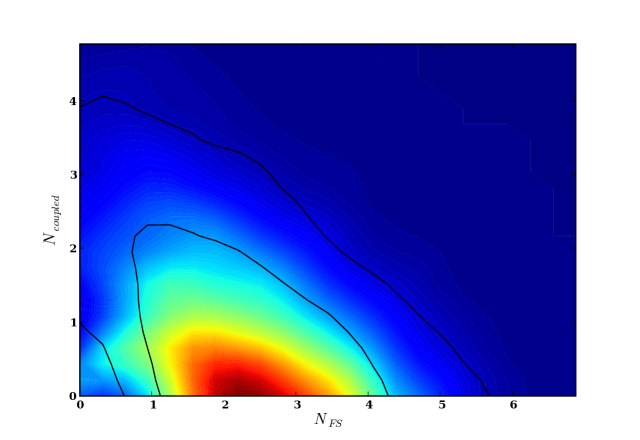
Figure 5: Sensitivity of WMAP3 + SDSS (LRG) + 2dF + HST + SNIa. The removal of the SDSS Main sample lowers the best fit point for $N_{FS}$ and signficantly weakens the constraints on a scenario with $N_{coupled}=3$ and $N_{FS}=0$.

It turns out that the piece of data responsible for favoring large $N_{FS}$ is the Main data sample from SDSS. With it removed (i.e., with the matter power given by the LRG SDSS dataset and 2dF dataset), the fit changes dramatically, as shown in Fig. 5. The new fit has a slight preference for values of $N_{FS}$ less than three: the best fit lies at $N_{FS}=2.5$, $N_{coupled}=0.1$.

Conversely, if we remove the LRG data from the fit, the best fit point moves all the way to $N_{FS}=5.2$, $N_{coupled}=0.1$, as can be seen in Fig. 6. Marginalizing over all other parameters including $N_{coupled}$ yields $N_{FS}=4_{-1.3}^{+2.2}$. Thus, it may be too early to conclude that the SDSS LRG and Main samples are consistent with each other. At least as implemented in COSMOMC, they pull the best-fit value of $N_{FS}$ in different directions, with the LRG sample favoring the standard values.

Our results show that if one chooses to rely on the LRG sample, one finds much less sensitivity to neutrino self-coupling: the point $N_{FS}=0$, $N_{coupled}=3$ lies inside the 2 $\sigma$ contour, while $N_{FS}=1$, $N_{coupled}=2$ lies on the 1 $\sigma$ contour. Thus, at present the bounds on coupled neutrinos from the global fit should perhaps be taken with caution.

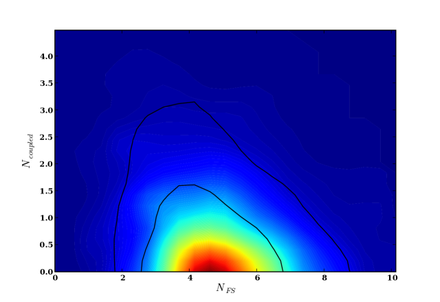
Figure 6: Sensitivity of WMAP3 + LSS from SDSS and 2dF + HST + SNIa. Compared to the previous figure, LRG data has been replaced with SDSS Main sample. SDSS main prefers larger $N_{FS}$ compared to LSS from LRG data sample.

IV.1.4 Adding the Lyman-$\alpha$ data.

We also repeat the analysis including the Lyman-$\alpha$ dataset in the fit. This dataset has been somewhat controversial . Our main reason for doing this calculation is to get an idea about the additional sensitivity that can be gained from this dataset, and also to further check consistency with the published analyses where this data is used.

We find that the overall sensitivity to coupled neutrinos is somewhat increased with the addition of this piece of data. Relative to the standard case of three free-streaming neutrinos, the case with a single coupled neutrino is disfavored at 1.8$\sigma$, the case with two coupled neutrinos is disfavored at 3.1$\sigma$ and, finally, the case with three coupled neutrinos is disfavored at 4.1$\sigma$. In other words, the addition of the Lyman-$\alpha$ data does bring further improvements in sensitivity, though not very large ones. The Lyman-$\alpha$ dataset does favor large values of $N_{FS}$, just like the SDSS Main sample, as also observed in Bell et al. (2006), Seljak et al. (2006). The comments at the end of the last Subsection apply here as well.

IV.2 Sensitivity of Planck

IV.2.1 Planck only

As already mentioned, the situation will improve markedly with the expected data from the Planck satellite. In this subsection, we describe the result of our MCMC analysis of Planck’s sensitivity.

We generate mock data for Planck in the all_l_exact data format of COSMOMC, using the best-fit point of WMAP3 as the “true” (seed) value and assuming flat Universe, $w=-1$ for the cosmological constant, and $N_{FS}=3.04$, $N_{coupled}=0$ for the numbers of neutrinos. The characteristics of the Planck detector (the beam size and the noise levels for temperature and polarization measurements) are given in Planck Collaboration . The relevant measurements will be done in three frequency channels of the High Frequency Instrument (HFI), 100, 143, and 217 GHz. In the literature Bowen et al. (2002); Bashinsky and Seljak (2004), the analyses have been done assuming an effective single channel for Planck. Ref. Bashinsky and Seljak (2004) in particular uses the sky coverage of $f_{sky}=0.80$, the detector noise for temperature $w_{T}^{-1/2}=40\mu\mbox{K}^{\prime}$, and for polarization $w_{P}^{-1/2}=56\mu\mbox{K}^{\prime}$ and the beam size $\theta_{b}=7^{\prime}$ (see Sect. V.1 for the definitions of these quantities). We have checked that these effective numbers (especially the value of $w_{P}^{-1/2}$) are in reasonably good agreement with these three-channel parameters of Planck Collaboration . The only substantial difference is that we believe it is more appropriate to take $f_{sky}=0.65$ .

Our analysis here parallels that of the last Subsection. We first fit the mock data in the several specific scenarios considered early, namely, varying the numbers of self-coupled neutrinos keeping the total neutrino number at three, and then varying the number of standard neutrinos assuming no self-coupled neutrinos. We compare the quality of the best fits in each case and observe how the cosmological parameters change to compensate for the effects of neutrino coupling. For our second analysis, we perform a global fit in the space of parameters $(N_{FS},N_{coupled},\Omega_{b}h^{2},\Omega_{c}h^{2},\theta,\tau,Y_{\rm He},n_{s},n_{\rm run},\log[10^{10}A_{s}])$. We then marginalize over the last 8 parameters to obtain the allowed region in the space of $N_{FS},N^{coupled}$.

$(N_{FS},N_{coupled})$	$\delta\chi^{2}$	C.L.	$\Omega_{b}h^{2}$	$\Omega_{c}h^{2}$	$\theta$	$\tau$	$Y_{\rm He}$	$n_{s}$	$n_{\rm run}$	$\log[10^{10}A_{s}]$	$\Omega_{\Lambda}$	Age/GYr	$\Omega_{m}$	$z_{re}$	$H_{0}$
$(3,0)$	–	–	$0.02246$	$0.10673$	$1.0417$	$0.089$	0.243	$0.952$	0.001	$3.03$	$0.76$	13.68	0.24	11.3	72.9
$(2,1)$	21.1	$4.2\sigma$	$0.02304$	$0.10485$	$1.0460$	$0.089$	0.262	$0.948$	0.016	$2.97$	$0.78$	13.49	0.22	11.3	75.5
$(1,2)$	85.5	$>8\sigma$	$0.02356$	$0.10273$	$1.0503$	$0.088$	0.277	$0.943$	0.030	$2.89$	$0.79$	13.31	0.21	11.1	78.3
$(0,3)$	197.5	$>8\sigma$	$0.02403$	$0.10097$	$1.0542$	$0.088$	0.281	$0.932$	0.039	$2.81$	$0.81$	13.11	0.19	11.0	81.5
$(1,0)$	91.7	$>8\sigma$	$0.02139$	$0.08096$	$1.0495$	$0.088$	0.298	$0.890$	-0.017	$2.95$	$0.70$	16.06	0.30	11.2	58.9
$(5,0)$	32.9	$5.4\sigma$	$0.02285$	$0.13327$	$1.0358$	$0.093$	0.162	$0.975$	0.006	$3.08$	$0.78$	12.16	0.22	11.4	84.2

Table 3: The same as in Table 1, but now fitting to the mock Planck dataset.

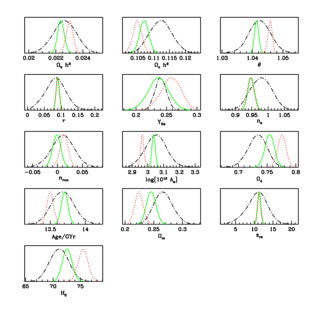
Figure 7: The improvement of sensitivity of Planck (solid) over the current data (dashed), assuming the standard scenario of three freely streaming neutrinos. The dotted curve illustrates how the parameters measured at Planck would shift assuming a single neutrino species is coupled. The current dataset is comprised of the data from WMAP3, SDSS Main and LRG, 2dF, HST, and SN Ia, plus the observational prior on $Y_{\rm He}$ (see text for details).

The results of the first set of calculations are tabulated in Table 3. The trends in the parameter shifts are similar to the case of WMAP3 – both $n_{s}$ and $A_{s}$ decrease while the physical baryon density increases as more neutrinos are coupled – but with Planck the shifts are much constrained. Moreover, the degeneracies are very efficiently broken and the quality of the best fits is significantly poorer in the coupled cases relative to the standard case. The scenario of a single coupled neutrino ($N_{FS}=2$, $N_{coupled}=1$) is disfavored at 4.2$\sigma$ relative to the standard one. The scenario with ($N_{FS}=5$, $N_{coupled}=0$) is disfavored at 5.4$\sigma$, while the other scenarios in the Table are ruled at greater than 8$\sigma$. Clearly, Planck’s sensitivity will be dramatically better than that of the current data.

The situation is graphically illustrated in Fig. 7, where the solid curves show the expected measurements at Planck and the dashed curves are those obtained with the combined current data (see Sect. IV.1.3) – both under assumption of three standard freely streaming neutrinos. The dotted curves show how the best-fit parameters shift if one instead fits the data under the assumption of a single coupled neutrino ($N_{FS}=2$, $N_{coupled}=1$). Clearly, Planck by itself will have errors that are significantly smaller than those of today’s experiments combined.

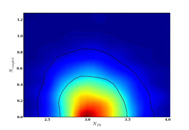
Figure 8: Expected sensitivity of Planck alone to $N_{FS}$, $N_{coupled}$.

The results of the second calculation show that this level of sensitivity persists for any direction in the $(N_{FS},N_{coupled})$ plane. The sensitivity contours in this plane are depicted in Fig. 8. We wish to stress two main results of this analysis: (i) the sensitivities of Planck to $N_{coupled}$ and $N_{FS}$ are similar, and (ii) for no direction in the plane $(N_{coupled},N_{FS})$ is there is a degeneracy between the two parameters. We will return again to the last point in Section V.1.

Our prediction for Planck’s sensitivity to the number of freely streaming neutrinos is asymmetric, $\Delta N_{\nu}=^{+0.5}_{-0.3}$. The lower error roughly agrees with that of Bashinsky and Seljak (2004), when the choice of higher $f_{sky}$ is taken into account, and Perotto et al. (2006) obtained with the Fisher matrix method. It is in reasonable agreement with what Perotto et al. (2006) finds with the MCMC method assuming no lensing of the CMB. We have investigated the effect of lensing on the sensitivity and we do not find the large effect of Perotto et al. (2006). Instead we find the bounds remain similar, slightly weaker for $N_{FS}$, slightly stronger for $N_{coupled}$. Notice that Bashinsky and Seljak (2004), considering Planck’s sensitivity to $N_{FS}$ with the Fisher analysis, also finds the effect of lensing small.

IV.2.2 Planck plus other cosmological data

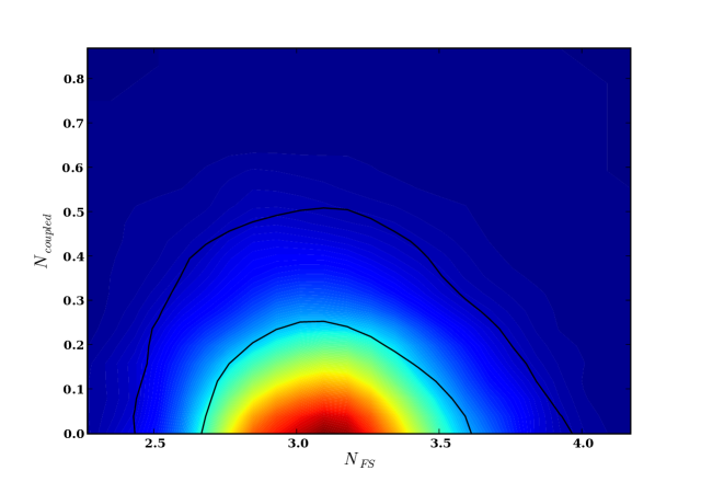
Figure 9: Sensitivity of Planck plus other cosmological data. The constraints on $N_{FS}$ are not much changed as compared with Planck alone, but the figure shows a factor of two potential improvement in $N_{coupled}$.

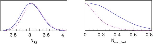
Figure 10: Sensitivity of Planck plus other cosmological data (dashed-dotted) vs. Planck only (solid). 1-d marginalized probabilities.

Lastly, we briefly consider what might be gained by combining Planck with the other cosmological data. For that, we run a combined fit to Planck, LRG and Main samples of SDSS, 2dF, the Type Ia supernova data and the Hubble constant measurements from the HST.

The result of the fit is shown in Fig. 9. The sensitivity to the number of freely streaming neutrinos is unaffected by the addition of the other data, while the sensitivity to coupled neutrinos improves by a factor of two. This can also be seen from the one-dimensional marginalized plots in Fig. 10.

One should, of course, not overinterpret this result. It should be kept in mind that the mock data for Planck was generated from the best-fit point of WMAP3 and we did not explore the dependence of the fit on this choice. Also, by the time Planck’s data is available, the other experiments could be updated. Nevertheless, the general lesson is that while most of the precision will come from Planck, the addition of the other data may lead to further tightening of the bounds.

V Discussion of the results and further numerical investigations.

The results of the previous Section indicate that Planck should constrain the numbers of coupled (and freely streaming) neutrino species much more accurately than what is possible today. In this Section, we make this statement more robust by investigating the following points:

• The sensitivity is an indication that not all of the effects of neutrino coupling could be compensated and that the residuals should be within the sensitivity reach of Planck’s instruments. We recall that in the last Section, we varied these parameters: $N_{FS}$, $N_{coupled}$, $\omega_{b}$, $\omega_{c}$, $\theta$, $\tau$, $n_{s}$, $n_{\rm run}$, $A_{s}$, $Y_{\rm He}$. We have omitted other cosmological parameters such as the curvature $\Omega_{curv}$, or the dark energy equation of state $w$. If varying these additional parameters introduced additional ways of compensating the effects of neutrino coupling, the bounds of the previous Section could be weakened. We need to show that this is not the case.

• We also made assumptions about the performance of Planck’s detector. We need to check the robustness of our results with respect to changing the characteristics of the detectors, such as the angular resolution and the detector noise levels. Put another way, we need to establish which multipoles $l$ are crucial for this measurement.

We will investigate these points using the Fisher matrix technique.

In addition to these practical issues, we will also investigate the issue of principle: what is the nature of Planck’s sensitivity to neutrino coupling? We do that by examining which effects of coupling cannot be compensated by adjusting the cosmological parameters.

V.1 The role of other cosmological parameters

As mentioned before, we will investigate the role of other cosmological parameters using the Fisher matrix technique. The idea is very simple: suppose that the likelihood function around the best-fit point is approximately gaussian. In this case, one can fix the parameters of the gaussian (in the case of an $N$ dimensional parameter space, an $N\times N$ symmetric matrix) by evaluating the likelihood function at $O(20)$ points, rather than at $10^{5}$ points, as in the case of mapping out the parameter space with MCMC.

The main reason for using this approximate method is speed Bowen et al. (2002). Obviously, the Fisher matrix method has its limitations, as for example, was recently discussed in Perotto et al. (2006). Still we believe that our usage of the Fisher matrix approximation – not to obtain the exact bounds but to investigate qualitative issues outlined above – is appropriate.

By expanding the log of the likelihood function to the second order in cosmological parameters $s_{i}$ around the maximum, one finds the standard expression:

$$F_{ij}=\sum_{l}\sum_{X,Y}\frac{\partial C_{l}^{X}}{\partial s_{i}}\mbox{Cov}^{-1}(\hat{C}_{l}^{X},\hat{C}_{l}^{Y})\frac{\partial C_{l}^{Y}}{\partial s_{j}}.$$ (10)

Here $\mbox{Cov}^{-1}$ is the inverse of the covariance matrix (to be defined shortly), and the $C_{l}^{X}$ are the power spectra in the temperature and polarization channels. We restrict ourselves to the temperature, $T$, $E$ polarized, and cross temperature-polarization $C$, power spectra. They are the only ones relevant for scalar perturbations.

The elements of the covariance matrix Seljak (1996); Zaldarriaga and Seljak (1997); Eisenstein et al. (1999), which give the errors of the corresponding measurements, are:

$$({\rm Cov}_{\ell})_{TT} = {2\over(2\ell+1)f_{\rm sky}}(C_{T\ell}+w_{T}^{-1}B_{\ell}^{-2})^{2},$$ (11)

$$({\rm Cov}_{\ell})_{EE} = {2\over(2\ell+1)f_{\rm sky}}(C_{E\ell}+w_{P}^{-1}B_{\ell}^{-2})^{2},$$ (12)

$$({\rm Cov}_{\ell})_{CC} = {1\over(2\ell+1)f_{\rm sky}}\left[C_{C\ell}^{2}+(C_{T\ell}+w_{T}^{-1}B_{\ell}^{-2})\right.$$ (13)

$$\left.\times(C_{E\ell}+w_{P}^{-1}B_{\ell}^{-2})\right],$$

$$({\rm Cov}_{\ell})_{TE} = {2\over(2\ell+1)f_{\rm sky}}C_{C\ell}^{2},$$ (14)

$$({\rm Cov}_{\ell})_{TC} = {2\over(2\ell+1)f_{\rm sky}}C_{C\ell}(C_{T\ell}+w_{T}^{-1}B_{\ell}^{-2}),$$ (15)

$$({\rm Cov}_{\ell})_{EC} = {2\over(2\ell+1)f_{\rm sky}}C_{C\ell}(C_{E\ell}+w_{P}^{-1}B_{\ell}^{-2}).$$ (16)

In these equations, $f_{sky}$ is the sky coverage, $w_{T}^{-1}$ and $w_{P}^{-1}$ specify the detector noise for temperature and polarization respectively, and $B_{\ell}^{-2}=e^{l(l+1)\theta_{b}^{2}/(8\ln 2)}$ is the beam smearing window function. Here $\theta_{b}$ is the full-width, half-maximum of the beam in radians, $w_{T}$ and $w_{P}$ are the quantities characterizing the detector noise level for temperature and polarization, respectively. For Planck, we take $\theta_{b}=7^{\prime}$, $w_{T}^{-1/2}=40\mu\mbox{K}^{\prime}$, and $w_{P}^{-1/2}=56\mu\mbox{K}^{\prime}$.

More precisely, the Fisher information matrix $F_{ij}$ is defined through derivatives of the likelihood function ${\cal L}(x,p)$ for data $x$ and model parameters $p$ as

$$F_{ij}\equiv\left\langle-\frac{\partial^{2}\ln{\cal L}(x,p)}{\partial p^{i}\partial p^{j}}\right\rangle_{x}.$$ (17)

The right-hand side of Eq. (17) is averaged over the data $x$, weighted by the probability ${\cal L}(x,p)$ of their observation in the fiducial model. Given this definition, the Cramér-Rao inequality states that the r.m.s. of the best-estimator for a parameter $p^{i}$ cannot be less than $\sqrt{({F^{-1}})^{ii}}$, as discussed, e.g., in Eisenstein et al. (1999).

Of course, to perform the average in general requires mapping out the likelihood function over the parameter space and we are back to the problem of computing the likelihood at $O(10^{5})$ points. We do not perform such mapping here. Instead, we simply assume the likelihood is close to gaussian, compute the matrix in Eq. (10), and use $\sqrt{({F^{-1}})^{ii}}$ as an estimate of a 1$\sigma$ error on the parameter $s_{i}$.

We consider the following set of cosmological parameters $(\omega_{m}/\omega_{r},\omega_{b},\Omega_{\rm de},N_{\nu}^{eff},N_{coupled},n_{s},\alpha_{s}$ $A_{s},Y_{\rm He},\tau,\omega_{\rm\nu},\Omega_{\rm c},w_{\rm de})$, replacing $N_{FS}$ with $N_{\nu}^{eff}=N_{FS}+N_{coupled}$ in our list of parameters. The first 10 parameters span the parameter space of our MCMC analysis of the last Section, while the last three are the new additions. We calculate the derivatives in Eq. (10) by symmetric finite differences about the best-fit cosmological parameters from the WMAP year three data. We compute the resulting 1$\sigma$ marginalized error on $N_{coupled}$ and $N_{\nu}^{eff}$ with all 13 parameters and then drop the last three parameters in turn. We also consider the effect of fixing the helium abundance $Y_{\rm He}$.

	Vary all	Fix	Fix $\omega_{\nu}=0$,	Fix $\omega_{\nu}=0$, $\Omega_{curv}=0$,	Fix $\omega_{\nu}=0$, $\Omega_{curv}=0$,
	13 params.	$\omega_{\nu}=0$	$\Omega_{curv}=0$	$w_{\rm de}=-1$	$w_{\rm de}=-1$, $Y_{\rm He}=0.24$
Error on $N_{coupled}$	0.31	0.31	0.31	0.29	0.28
Error on $N_{\nu}^{eff}$	0.38	0.38	0.38	0.35	0.32

Table 4: The Fisher matrix estimate of the 1$\sigma$ error on $N_{coupled}$ and $N_{\nu}^{eff}$. The effects of fixing neutrino mass, curvature, dark energy equation of state, and the Helium fraction are considered.

The results are shown in Table 4. We see that keeping the curvature and the neutrino mass fixed to zero is completely justified. Moreover, the effect of varying the dark energy equation of state is also quite small ($\sim 7$% for $N_{coupled}$ and $\sim 9\%$ for $N_{\nu}^{eff}$), as is the effect of varying $Y_{\rm He}$ ($\sim 4$% for $N_{coupled}$ and $\sim 9\%$ for $N_{\nu}^{eff}$). Thus, practically speaking, we are justified in our choice of the 10 cosmological parameters used in our MCMC calculations, as the other three parameters do not change our qualitative conclusions about Planck’s sensitivity to the number of coupled neutrinos. In addition, though the Fisher analysis shows that the effects of $Y_{\rm He}$ on the errors of $N_{coupled}$ and $N_{\nu}^{eff}$ are fairly minimal, we include $Y_{\rm He}$ as a parameter in our MCMC with priors consistent with astrophysical observations as described in Sect. IV.1.3.

V.2 The compensation mechanism and the nature of Planck’s sensitivity

We now wish to establish the nature of Planck’s sensitivity to neutrino self-coupling. By this we mean showing which effects of self-coupling cannot be entirely compensated by adjusting the cosmological parameters and how the residual differences compare to the corresponding errors. The latter, as we saw in the previous subsection, are set by a combination of the cosmic variance and the resolution/sensitivity of the apparatus. Equipped with our numerical results, we are now able to explicitly see the compensation mechanism in action.

For this, we turn to Table 3. The best-fit parameters listed in the Table are precisely those which compensate the effects of neutrino coupling most efficiently within each scenario. Indeed, we recall that while the mock data is always generated under the assumptions of three freely streaming neutrinos, for each of the scenarios listed in the Table, the MCMC code attempts to find the best fit possible within the framework of that particular scenario. The code varies the values of the cosmological parameters until the closest agreement is found.

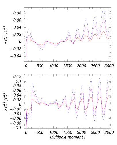
Figure 11: The relative residual differences in temperature and polarization power spectra for 1, 2, and 3 coupled neutrinos (in order of deviation from zero) that remain after the cosmological parameters are adjusted in each of the scenarios (as shown in Table 3).

The compensation turns out to be very efficient. One way to illustrate it is to plot the relative differences of the temperature and polarization power spectra in the scenarios of coupled vs. freely streaming neutrinos that remain after the cosmological parameters are adjusted. This is done in Fig. 11, where we show the situations for 1, 2, and 3 coupled neutrinos. We can see that, unlike the differences shown in Fig. 1 which were in tens of percent, these residual differences are only at the level of 1-3%.

We further observe that below the multipole number of $l\sim 1300$ the residuals have no clear structure, while above they develop a shape of periodic oscillations, as a consequence of the phase shift, Eq. (7).

In terms of the sensitivity of Planck, the physically relevant quantities are not the relative differences in the $C_{l}$’s just shown, but the ratios of the differences to the corresponding errors. The errors are given by the elements of the covariance matrix, Eqs. (11-16). We can then consider at each $\ell$ the quantities

$$(\delta\chi_{\ell})^{XX}\equiv\frac{\Delta C_{l}^{X}}{\sqrt{({\rm Cov}_{\ell})_{XX}}},$$ (18)

where $X$ runs over $T$, $E$, and $C$, and $\Delta C_{l}^{X}$ are again the differences between the power spectra of the reference model ($N_{FS}=N_{\nu}^{eff}=3$) and the best-fit power spectra in a scenario with self-coupled neutrinos.

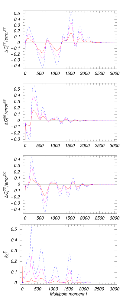
Figure 12: The quantities $(\delta\chi_{\ell})^{X}$ and $(\delta\chi_{\ell}^{2})$ defined in Eqs. 18 and 19. They illustrate the ratios of the residual discrepancies at each $\ell$ to the corresponding errors, as explained in the text. The residual discrepancies at $\ell\lesssim 1300$ play a key role.

The quantities $(\delta\chi_{\ell})^{X}$ are plotted in Fig. 12 (the top three panels). In the last panel of the figure, we plot the quantity

$$(\delta\chi_{\ell}^{2})\equiv\sum_{X,Y=\{T,E,C\}}(\Delta C_{\ell}^{X})({\rm Cov}_{\ell})_{XY}^{-1}(\Delta C_{\ell}^{Y}),$$ (19)

which is nothing but the contribution of a given multipole $\ell$ to the $\chi^{2}$. These Figures are very instructive, for they show that statistically significant deviations occurs for $\ell\lesssim 1300$, and have no clear structure. The higher multipoles which exhibit clear effects of the phase shift in Fig. 11 turn out to be of relatively minor importance.

This is further seen when we consider the effects of the expected detector resolution and noise on the $1\sigma$ errors in $N_{coupled}$. In Figs. 13, 14, we show the change in sensitivity as a function of detector characteristics, obtained a Fisher analysis. The rate at which increased resolution and lower noise improve the sensitivity to $\Delta N_{coupled}$ is rather modest. Decreasing the noise by an order of magnitude, for example, improves the sensitivity by less than a factor of two. In addition, we consider the sensitivity of a hypothetical experiment which measures all multipoles with $\ell<\ell_{max}$ within cosmic variance; we see in Fig. 15 that sensitivity to multipoles $\ell_{max}\lesssim 1000$ is sufficient to measure $\Delta N_{coupled}=0.3$, and implies that Planck’s high sensitivity to neutrino free-streaming does not depend on the high $\ell$ multipoles. It also implies that our qualitative predictions for Planck have a high degree of robustness, as the sensitivity does not depend strongly on the high $\ell$ properties of the detector.

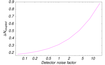
Figure 13: $1\sigma$ sensitivity of Planck (calculated with a Fisher matrix) to $\Delta N_{coupled}$ as a function of the detector noise. A noise factor of one corresponds to the sensitivity chosen in the main analysis ($w_{T}^{-1/2}=40\mu K^{\prime}$, $w_{P}^{-1/2}=56\mu K^{\prime}$).

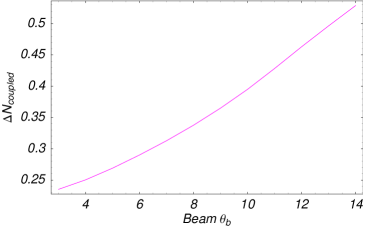
Figure 14: $1\sigma$ sensitivity of Planck (calculated with a Fisher matrix) to $\Delta N_{coupled}$ as a function of the detector resolution. The resolution chosen in the main analysis is $7^{\prime}$.

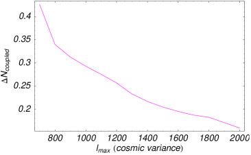
Figure 15: $1\sigma$ sensitivity of a hypothetical CMB experiment to $\Delta N_{coupled}$ as a function of the maximum multipole, $l_{max}$, measured to within cosmic variance. Multipoles with $l>l_{max}$ are discarded.

One characteristic of Planck that proves crucial is the simultaneous measurement of both temperature and polarization. This makes it possible for Planck to constrain $N_{coupled}$ down to 0.5 at 1$\sigma$ level even if $l_{\rm max}$ is only 800. In comparison, we saw that WMAP3 places virtually no constraint on the number of self-coupled neutrinos. The difference is the relatively poor quality of the polarization measurements at WMAP, as well as the temperature measurements for $500\lesssim l\lesssim 800$, where Planck is cosmic variance limited.

VI Constraints on neutrino interactions

Since we have shown that even a single interacting neutrino or a single extra neutrino will be observed or excluded to high precision with Planck, we consider the implications for models of neutrino-scalar interactions, including neutrino dark energy. Before turning to the specific models, we first review general constraints on the couplings $g$ from Majorana neutrino-scalar interactions which will be possible with Planck data.

The loss of neutrino free-streaming and production of additional relativistic degrees of freedom as a result of neutrino-scalar coupling have been considered in Ref. Chacko et al. (2004). We summarize and reformulate the constraints here; a more complete treatment is left to the appendix.

For a Majorana mass term, the relevant interactions $\nu\nu\leftrightarrow\phi\phi$, $\nu\nu\leftrightarrow\nu\nu$, and (if $m_{\phi}>2m_{\nu}$) $\nu\nu\leftrightarrow\phi$. The last interaction is often most constraining on the coupling $g$, and its rate is

$$\Gamma(\nu\nu\leftrightarrow\phi)\sim\frac{g^{2}}{16\pi}\frac{m_{\phi}}{T}m_{\phi}$$ (20)

for $m_{\phi}<T$. This rate can also be described from on resonant s-channel scattering; see the appendix for details. The $m_{\phi}/T$ factor accounts for the boost from the rest frame of the scalar. This rate increases as the temperature decreases, and will cause $\phi$ to decay to neutrinos, increasing $N_{\nu}^{eff}$, once $m_{\phi}$ drops below $T$, provided $g\gtrsim 10^{-13}(T_{rec}/m_{\phi})$.

If, on the other hand, $m_{\phi}$ remains relativistic through recombination, this same process may tightly couple the neutrino to the scalar, removing neutrino free-streaming. The $2\rightarrow 1$ process can only occur in a small region of phase space which depends on the angle between the incoming neutrinos, $\theta\sim m_{\phi}/T$. In order to isotropize the neutrino momentum, therefore, this process must occur $N=(T/m_{\phi})^{2}$ times. We require then $\Gamma(\nu\nu\leftrightarrow\phi)>NH(T_{rec})$ Chacko et al. (2004). The equilibration occurs before recombination if $g\gtrsim 10^{-13}$ for $m_{\phi}\sim T_{rec}$, and becoming less restrictive with dropping $m_{\phi}$ by the factor $(T_{rec}/m_{\phi})^{2}$.

The exception is if scattering of $\phi$’s through a $\phi^{4}$ interaction may be fast enough to isotropize the scalar momentum in between decays and inverse decays. Then the constraint is transmuted to $\Gamma(\phi\phi\leftrightarrow\phi\phi)>\Gamma(\nu\nu\leftrightarrow\phi)>H(T_{rec})$, which implies that if $\lambda_{\phi}^{2}T>T^{2}/M_{pl}$, where $\lambda_{\phi}$ is the coupling of the $\phi^{4}$ interaction, and if $g^{2}m_{\phi}^{2}/T>T^{2}/M_{pl}$, then the neutrinos will be strongly coupled with the scalars. The equilibration then occurs before recombination if

$$g\gtrsim 10^{-14}(T_{rec}/m_{\phi})$$ (21)

and

$$\lambda_{\phi}\gtrsim 10^{-14}.$$ (22)

$2\leftrightarrow 2$ interactions offer complementary constraints to the decay-inverse decay processes. If both neutrinos and scalars are relativistic at decoupling, the rate for $\nu\nu\leftrightarrow\nu\nu$ is given by

$$\Gamma(\nu\nu\leftrightarrow\nu\nu)\sim\frac{g^{4}}{16\pi}T,$$ (23)

and is competitive with $\nu\nu\leftrightarrow\phi\phi$, so that if $g\gtrsim 10^{-7}$ neutrinos and scalars will be tightly coupled. If $m_{\phi}\gtrsim T_{rec}$, however, the constraints on $g$ are relaxed by $T/m_{\phi}$, due to propagator suppression from the scalar.

We have assumed everywhere that $m_{\nu}\ll T_{rec}$. If $g\gtrsim 10^{-5}$ and $m_{\nu}>T_{rec},\mbox{ }m_{\phi}$, the neutrinos will annihilate to the scalars, producing a “neutrinoless” universe Beacom et al. (2004); for this process, $N_{\nu}^{eff}$ is an evolving function of redshift as the neutrinos annihilate. We do not consider this scenario further in this paper.

We briefly discuss the constraints from BBN. The precise upper bound on the effective number of neutrinos is somewhat controversial and dependent on the particular set of constraints from data utilized, but is on the order of $N_{\nu}^{eff}\lesssim 4.5$ Cyburt et al. (2005). Any additional scalar degrees of freedom brought into equilibrium before BBN will contribute $\delta N_{\nu}^{eff}=4/7$. One scalar alone brought into thermal equilibrium before BBN, then, will not upset the current bounds. If the theory contains multiple scalars, however, there will be constraints already from BBN on the coupling $g$ from $\nu\nu\leftrightarrow\phi$ and $\nu\nu\leftrightarrow\phi\phi$ coming from demanding that these processes not recouple until $T<T_{BBN}$.

If these processes are brought into equilibrium after the neutrino processes decouple from the heat bath at $T\sim 1\mbox{ MeV}$, they may still affect the value of $N_{\nu}^{eff}$ measured by the CMB Chacko et al. (2004, 2005). For example, it may be possible that new particle states (e.g., scalars, sterile neutrinos) are populated by recoupling after BBN and then annihilate when the temperature drops below their masses (but still before the CMB decoupling). In this scenario, while the annihilation step occurs at constant entropy, the recoupling does not. In the approximation when the former occurs at constant energy, the value of $N_{\nu}^{eff}$ measured by the CMB is given by Eq. (8) of Chacko et al. (2005). In general, for a given model, accurate analysis of recoupling may be required.

We summarize the future constraints from Planck given no deviation from standard relativistic energy density and neutrino free-streaming in Table 5.

process	$m_{\phi}$	constraint	Effect on CMB
$\nu\nu\leftrightarrow\phi$	$T_{rec}>m_{\phi}$	$g\lesssim 10^{-13}\left(1\mbox{ eV}/m_{\phi}\right)^{2}$	Remove free-streaming
	$T_{rec}<m_{\phi}$	$g\lesssim 10^{-13}\left(m_{\phi}/1\mbox{ eV}\right)^{1/2}$	Increase $N_{\nu}^{eff}$
$\nu\nu\leftrightarrow\nu\nu$	$T_{rec}>m_{\phi}$	$g\lesssim 10^{-7}$	Remove free-streaming
	$T_{rec}<m_{\phi}$	$g\lesssim 10^{-7}\left(m_{\phi}/1\mbox{ eV}\right)$	Remove free-streaming
$\nu\nu\rightarrow\phi\phi$	$m_{\phi}<T_{rec}<m_{\nu}$	$g\lesssim 10^{-5}$	Increase $N_{\nu}^{eff}$

Table 5: Constraints on the effective coupling $g$ of a Majorana neutrino with a scalar, if the Planck satellite observes no extra, non-standard relativistic degrees of freedom or strong neutrino-scalar interactions.

VII Some implications for models

VII.1 Models of Neutrino Dark Energy

Models of neutrino dark energy are typically characterized by a coupling between a singlet neutrino and a light scalar field of the form given in Eq. 2. An important difference between the standard see-saw and the MaVaN scenario is that $m_{N}$ is a continuously evolving parameter, since the vev of the singlet scalar, $\langle\phi\rangle$, varies as the universe cools.

The evolution of $\langle\phi\rangle$ results from finite temperature effects in the scalar potential; the background neutrino energy density acts as a source for the scalar field, and may displace $\langle\phi\rangle$ from the value dictated by its zero-temperature potential, $V_{0}(\phi)$:

$$V(\phi) = V_{0}(\phi)+\rho_{\nu}(\phi)$$ (24)

$$\simeq \frac{1}{2}m_{\phi}^{2}\phi^{2}+\frac{7\pi^{2}}{120}T^{4}+\frac{m_{\nu}^{2}(\phi)T^{2}}{24},$$

where $m_{\nu}$ is the light mass eigenstate resulting when the sterile neutrino is integrated out:

$$m_{\nu} = \frac{m_{D}^{2}}{m_{N}}$$ (25)

$$= \frac{m_{D}^{2}}{\lambda\langle\phi\rangle}.$$

This is a self-consistent formalism provided that the sterile neutrino remains thermally unpopulated (and hence effectively integrated out) in the early universe; it was shown in Weiner and Zurek (2006) how this can be done with Planck suppressed operators between the scalar and electrons. In addition, in a theory with the full flavor structure of three generations, $m_{\nu}$ must correspond to the lightest mass eigenstate, which is still relativistic in the universe today, so that the neutrino dark energy does not clump and become unstable Afshordi et al. (2005).

As was shown in Sect. II, the mass eigenstate couples to the scalar through the Majoran interaction, ${\cal L}=g\phi\nu\nu$, where $g\sim\lambda(m_{D}/m_{N})^{2}$. Minimizing eqn. 24,

$$m_{N} = \lambda\langle\phi\rangle$$ (26)

$$= m_{D}\sqrt{\frac{\lambda T}{m_{\phi}}}$$

Hence, we have a temperature dependent coupling $g$.

How can MaVaNs be detected with Planck? Planck will be sensitive to couplings g, through $\nu\nu\leftrightarrow\nu\nu$, of size $g\gtrsim 10^{-7}$; these couplings may be small enough to lead to possible detection or interesting constraints on MaVaNs with Planck. We conclude, using $m_{N}$ from eqn. 26

$$g=\frac{m_{\phi}}{T},$$ (27)

implying that the neutrinos will form a tightly coupled fluid down to recombination temperatures, $T\sim 0.1\mbox{ eV}$, unless

$$m_{\phi}\lesssim 10^{-8}\mbox{ eV}.$$ (28)

For scalars in these mass ranges, Planck will be able to detect MaVaNs.

What are natural parameters and typical scalar masses for the theory? We consider a generic class of MaVaN models laid out in Fardon et al. (2004, 2006). All energy scales in MaVaN models are characterized by the dark energy scale, $\Lambda\sim 10^{-2.5}\mbox{ eV}$. All parameters in the model, including $m_{D}$ and UV cutoff of the neutrino sector, are characterized by meV scale physics, in contrast to the traditional see-saw, which is characterized by a sterile neutrino at the GUT scale. Radiative corrections will drive the scalar mass to the cutoff of the theory, implying that without an unnatural fine-tuning, the scalar mass should not be much lighter than the cutoff of the theory at a meV. A superpotential which radiatively controls the scalar mass is simply the see-saw, eqn. 2, with all the fields promoted to superfields:

$$W=\lambda\phi NN+yHLN.$$ (29)

Assuming $\langle|N|\rangle=0$, the superpotential generates no tree-level mass term for $\phi$. A mass is generated radiatively for $\phi$, however, through a 1-loop diagram with an active and sterile sneutrino in the loop so that

$$m_{\phi}^{2}\sim\frac{\lambda^{2}m_{D}^{2}}{16\pi^{2}}\log\Lambda^{2}/m_{D}^{2}$$ (30)

where $\Lambda$ is the UV cutoff of the neutrino sector, typically around an eV. We can see that loop corrections will generically generate a mass for the scalar, $m_{\phi}\sim\lambda m_{D}$.

Besides the loop corrections of Eq. (30) one has to keep in mind corrections mediated by gravity. The natural size of gravity-mediated corrections to the scalar mass from supersymmetry broken at the TeV scale is $\sim F/M_{pl}\sim 10^{-3}$ eV, or some five orders of magnitude above the bound in Eq. (28).

$\lambda$ and $m_{D}$ are themselves constrained by the requirement that MaVaNs produce dark energy. In particular, it was shown Fardon et al. (2006) that a mass term appears for $|N|$ through radiative corrections of size $-\lambda^{2}m_{D}^{2}$, as it does for $|\phi|$, but with the opposite sign. This implies a false minimum at $\langle|N|\rangle=0$, with a true minimum at $\langle|N|\rangle\sim m_{D}/\lambda$ ; the energy difference between the true minimum of the potential and $\langle|N|\rangle=0$ is the dark energy density,

$$\rho_{\Lambda}\sim m_{D}^{4}/\lambda^{2}\sim 10^{-10}\mbox{ eV}^{4}$$ (31)

and, using $m_{\phi}\sim\lambda m_{D}$ from naturalness, we find that the only underlying free parameter is the coupling $\lambda$: $m_{\phi}\sim\lambda m_{D}\sim\lambda^{3/2}10^{-2.5}\mbox{ eV}$. In terms of the Lagrangian parameter $\lambda$, then, Planck will be able to constrain the coupling to be

$$\lambda\lesssim 10^{-5.5}.$$ (32)

Since $\lambda$ is a parameter typically envisioned to be not much smaller than 1, the reach of Planck is considerable. Of course, these constraints on Lagrangian parameters depend on naturalness requirements; the direct (more model independent) constraint is expressed in terms of the scalar mass in eqn. 28.

The same parameter $\lambda$ enters into matter effects in neutrino oscillation experiments, studied in, e.g., Kaplan et al. (2004); Zurek (2004); Barger et al. (2005); Cirelli et al. (2005); Blennow et al. (2005). There it was shown that the shift of the neutrino mass due to earth size matter effects is

$$\Delta M=1\mbox{ eV}\left(\frac{\lambda}{10^{-1}}\right)\left(\frac{\alpha_{N}}{10^{-2}}\right)\left(\frac{\rho_{N}}{\rho_{N}^{0}}\right)\left(\frac{10^{-6}\mbox{ eV}}{m_{\phi}}\right)^{2},$$ (33)

where $\alpha_{N}$ is a Planck suppressed coupling between nucleons and $\phi$, and $\rho_{N}^{0}=3\mbox{g/cm}^{3}$ is the earth energy density. Neutrino oscillation experiments in earth typically cannot reach sensitivities to mass scales smaller than $10^{-1}-10^{-3}\mbox{ eV}$. From this, we can can see that Planck and neutrino oscillation experiments are complimentary probes of neutrino dark energy. Neutrino oscillation experiments are efficient at detecting effects in the low $m_{\phi}$ region of parameter space; using the naturalness requirement, $m_{\phi}\sim\lambda m_{D}$, and the dark energy requirement, $m_{D}^{4}/\lambda^{2}\sim\rho_{\Lambda}$,

$$\Delta M=1\mbox{ eV}\left(\frac{\alpha_{N}}{10^{-2}}\right)\left(\frac{\rho_{N}}{\rho_{N}^{0}}\right)\left(\frac{10^{-7}\mbox{ eV}}{m_{\phi}}\right)^{4/3}.$$ (34)

Planck, on the other hand, can probe the large $m_{\phi}$ region according to eqn. 28.

VII.2 Late time neutrino masses

In models of late time neutrino masses Chacko et al. (2004, 2005), $\phi$ carries a $U(1)$ charge, which has a low scale $f$ of symmetry breaking. Since the mass eigenstate in the operator of the form $g\phi\nu\nu$ only acquires a mass once the $U(1)$ is broken (exactly as in the Higgs mechanism), the neutrinos only gain their masses at late time. For a low-energy Majorana mass term, we expect $g\sim m_{\nu}/f$, as shown in Sect. II. We conclude then that Planck will be able to probe scales of neutrino mass generation:

$$f\lesssim\begin{array}[]{cc}1\mbox{ MeV}&m_{\phi}<2m_{\nu}\\ 1\mbox{ TeV}&m_{\phi}>2m_{\nu}\end{array},$$ (35)

assuming $m_{\nu}\sim 0.1\mbox{ eV}$. Hence Planck may probe TeV scale neutrino mass generation.

VIII Conclusions

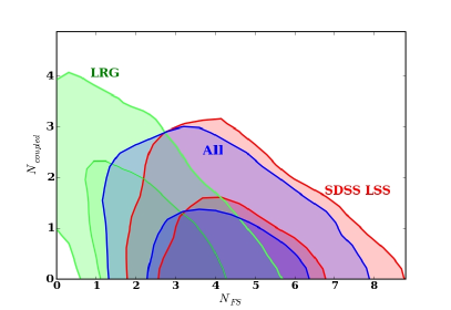
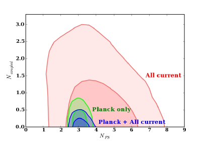
Figure 16: Summary of the bounds on the numbers of free-streaming and coupled neutrinos from the current data (left) and the simulated Planck data (right). For the case of the current data, the Large Red Galaxy (LRG) dataset from SDSS yields a region that differs significantly from what is obtained with the Main SDSS dataset. The combined fit is also shown. The sensitivity of Planck to the numbers of both freely streaming and coupled neutrinos will be a dramatic improvement over that of all present-day experiments combined (compare “Planck only” and “All current” on the right). If Planck’s data is combined with today’s data, further improvement on the constraints are expected.

We have considered in this paper the effect of neutrino interactions on the CMB, both through removal of neutrino free-streaming and the thermalization of extra relativistic degrees of freedom. The constraints from the current data are shown in Figs. 4, 5 and 6; those expected to be obtained with Planck are depicted in Figs. 8 and 9. These constraints are summarized in Fig. 16.

The current data disfavors 3 non-free-streaming neutrinos at the 3.5$\sigma$ level, however, this exclusion is not without some controversy. The exclusion comes from the SDSS Main data set (and also from the Lyman-$\alpha$ forest data), which favors five free-streaming neutrinos. We have seen that the LRG SDSS dataset instead favors close to three free-streaming neutrinos, in agreement with the standard model expectations, but has little sensitivity to coupled neutrinos.

We have shown that Planck will be able to resolve the present controversy. Planck alone will be capable of excluding a single interacting neutrino at the 4.2$\sigma$ level. Thus we expect sensitivity to models of neutrino mass and neutrino dark energy which is currently unavailable. Models of Mass-Varying Neutrinos, for example, in many regions of parameter space, predict only a single strongly coupled neutrino. Likewise, models of neutrino mass may have a flavor structure such that only one or two of the neutrinos is strongly enough coupled to the scalar to remove neutrino free-streaming at the CMB epoch. For the MaVaNs models, the reach of Planck will be considerable, probing the scalar masses down to $m_{\phi}\sim 10^{-8}$ eV, thus covering the parameter values favored by naturalness.

In the case of extra thermalized neutrinos or scalars, the current constraints depend on which data sets are chosen in the analysis, and in any case the errors encompass multiple neutrinos; as a result, the current data are not conclusive on the total radiation density at the CMB epoch. By contrast, Planck alone will determine the radiation content to $\Delta N_{\nu}=^{+0.5}_{-0.3}$.

The nature of the neutrino mass generation mechanism and beyond-the-standard-model neutrino interactions is currently unknown. The coupling between a neutrino and a light scalar in a Majoron interaction term of the form $g\phi\nu\nu$ can be as small as $g\sim 10^{-13}$ (depending on the mass of the scalar) while still being large enough to remove neutrino free-streaming and make an imprint on the CMB. The constraints (and potential for future detection) considered in this paper should be a guide to model builders when considering potential signals from future CMB experiments. It has been challenging to test neutrino properties in terrestrial experiments, and the nature of the mechanism which generates neutrino mass remains unknown; future CMB experiments may have the tools to unmask its origin.

Appendix A On Resonant Production

In this section we perform a more rigorous derivation of the results of Sect. VI.

Consider a “test” neutrino traveling through a neutrino gas. We need to know how far it travels before appreciably changing the direction of its momentum, i.e., given the initial momentum of order $T$, when the particle’s momentum in the transverse direction becomes order $T$. The rate for this process needs to be compared to the expansion rate of the universe, given by $\sim T^{2}/M_{pl}$ in the era of radiation domination.

Let us consider the scattering of two neutrinos, $\nu\nu\rightarrow\nu\nu$, and start with the $t$-channel exchange of $\phi$. In this case, for light $\phi$ ($m_{\phi}\ll T$) the cross-section is strongly forward peaked (the well-known property of Rutherford scattering). The situation is well-known in plasma physics. The build-up of transverse momentum happens mostly as a result of many small-angle scattering events, rather than a single large-angle event. The multiple scattering events result in a random walk process for the transverse momentum $p_{T}$, so that the rate of change of $p_{T}^{2}$ is given by

$$\frac{dp_{T}^{2}}{dt}\sim\int d(\cos\theta)\frac{d\sigma}{d\cos\theta}nv_{rel}p_{\theta}^{2}.$$ (36)

Taking $v_{rel}\sim 1$, $p_{\theta}^{2}\sim T^{2}\theta^{2}$, $n\sim T^{3}$ and $d\sigma/d\cos\theta\sim g^{4}/(16\pi)T^{2}(T^{2}\theta^{2}+m_{\phi}^{2})^{-2}$, we get

$$\frac{dp_{T}^{2}}{dt}\sim\frac{g^{4}}{16\pi}T^{3}\ln(T/m_{\phi}).$$ (37)

The small-angle behavior of the cross section is regulated by the mass of the scalar field. In plasma physics, the logarithm similar to that in the above equation (“the Coulomb logarithm”) is regulated by plasma screening effects.

The rate for the process needs to be compared to $T^{2}\times T^{2}/M_{pl}$ (“momentum exchange of order $T$ by the time when the temperature equals $T$”). We get that neutrinos are streaming freely at recombination when

$$g\lesssim(T_{\rm rec}/M_{pl})^{1/4}\times(16\pi/\ln(T_{\rm rec}/m_{\phi}))^{1/4}.$$ (38)

The 1/4 power makes the coefficient (the second term) of order one for a wide range of $m_{\phi}$, hence for the purpose of this estimate we can drop it. The order of magnitude is set by the ratio $(T_{\rm rec}/M_{pl})$. For the temperature $O(eV)$ one thus finds the neutrinos are not coupled by the $t$-channel scalar exchange if

$$g\lesssim 10^{-7}.$$ (39)

The 1/4 power also means that when the $t$ channel process is dominant it is reasonable to treat neutrinos as tightly coupled on all scales, not just the sound horizon at the CMB decoupling. Indeed, even considering scales 100 times smaller than the sound horizon only changes the bound on $g$ by about a factor of 3.

If $m_{\phi}>T$, the situation is different. The momentum exchange occurs via large-angle scattering and the cross section is set by $T^{2}/m_{\phi}^{4}$, so that

$$g\gtrsim(T_{\rm rec}/M_{pl})^{1/4}(m_{\phi}/T_{\rm rec}).$$ (40)

The interaction decouples as the temperature drops, a characteristic feature of nonrenormalizable interactions. Indeed, at temperature $T\ll m_{\phi}$ the $\phi$ field can be integrated out, resulting in an effective 4-fermion vertex.

We now consider $\nu\nu\rightarrow\nu\nu$ scattering via the $s$-channel process. In this channel, an important possibility is the scattering on-resonance. When it is open, it can increase the sensitivity to $g$ by orders of magnitude, as we will see next.

For $m_{\phi}<T$, the resonance condition is satisfied when the relative angle $\theta_{12}$ between the two incoming neutrinos, 1 and 2, is small, so that $s=E_{1}E_{2}(1-\cos\theta_{12})=m_{\phi}^{2}$, or $\theta_{12}\sim m_{\phi}/T$. The relative velocity $v_{rel}$ is given by $\theta_{12}$. The cross section in the center-of-mass frame is given by the relativistic Breit-Wigner form,

$$\sigma_{\rm CM}\sim\frac{\pi}{m_{\phi}^{2}}\frac{s\Gamma_{\phi}^{2}}{(s-m_{\phi}^{2})^{2}+s^{2}\Gamma_{\phi}^{2}/m_{\phi}^{2}},$$ (41)

where $\Gamma$ is the width of the resonance, given by the rate of decay of $\phi$ in its rest frame, $\Gamma_{\phi}=g^{2}m_{\phi}/(16\pi)$. The cross section has a peak value $\sim\pi/m_{\phi}^{2}$. In the frame of the universe, the cross section is reduced by a factor of $m_{\phi}/T=\theta_{12}$ (since it is boosted in the direction perpendicular to the direction of the colliding momenta in the center-of-mass frame).

Collecting all the factors, we obtain

$$\frac{dp_{T}^{2}}{dt}\sim m_{\phi}^{-2}\theta_{12}n_{res}\theta_{12}T^{2}\theta_{12}^{2},$$ (42)

where $n_{res}$ is the number density of neutrinos on which the test neutrino scatters resonantly. It can be estimated from the phase space as $\sim Tm_{\phi}\Gamma_{\phi}=g^{2}Tm_{\phi}^{2}/(16\pi)$. Hence,

$$\frac{dp_{T}^{2}}{dt}\sim\frac{g^{2}}{16\pi}\frac{m_{\phi}^{4}}{T}.$$ (43)

The result in Eq. (43) has a simple physical interpretation Chacko et al. (2004), as a resonant production of the $\phi$ particles, $\nu\nu\rightarrow\phi$, completely analogous to the $Z$-boson production at LEP. Indeed, the rate can be most easily computed in the opposite direction: the decay of $\phi$ boosted into the frame of the universe is $g^{2}m_{\phi}^{2}/T/(16\pi)$. To get the momentum exchange rate, one recalls that for each scattering event, one has $p_{T}\sim m_{\phi}$.

The crucial feature of the resonant process is the dependence on $g^{2}$, rather than $g^{4}$, since as we saw the reference values of $g$ are in the $10^{-7}$ range. Instead of Eq. (38) one has

$$g \lesssim (4\pi^{1/2})(T_{\rm rec}/M_{pl})^{1/2}\times(T_{\rm rec}/m_{\phi})^{2}$$ (44)

$$\lesssim 10^{-13}(T_{\rm rec}/m_{\phi})^{2}.$$

For $m_{\phi}\gtrsim 10^{-3}$ eV this constraint is stronger than that in Eq. (38). Otherwise, the integral over the nonresonant part of the phase space dominates, giving a bound similar to Eq. (38).

So far, our discussion has been in complete agreement with Ref. Chacko et al. (2004). We now point out some differences and make additional observations.

As noted in Chacko et al. (2004), in the models where the light scalar $\phi$ is the Goldstone boson there is a possibility to produce $\phi$ via the $s$-channel diagram with the heavy scalar $\rho$ (the radial mode) in the intermediate state, $\nu\bar{\nu}\rightarrow\rho\rightarrow\phi\phi$. Just like the process $\nu\nu\rightarrow\phi\rightarrow\nu\nu$ considered above, this process is most efficient at producing the $phi$ particles on resonance, i.e., at the point in the history of the universe when the temperature equals $\sim m_{\rho}$. Unlike the result given in Eqs. (28) and (29) of Chacko et al. (2004) we estimate the rate of this process treating it as $\nu\nu\rightarrow\rho$

$$\Gamma\sim\frac{g^{2}}{32\pi}m_{\rho}.$$ (45)

Comparing it with $T^{2}/M_{pl}=m_{\rho}^{2}/M_{pl}$ we find that unless

$$g \lesssim 4(2\pi)^{1/2}(m_{\rho}/M_{pl})^{1/2}$$ (46)

$$\lesssim 10^{-13}(m_{\rho}/T_{\rm rec})^{1/2}$$

the Goldstone degree of freedom will be populated. If this occurs before the neutrinos decouple (i.e., if $m_{\rho}\gg 1$ MeV), the number of effective neutrino degrees of freedom at BBN will be $3+4/7N_{G}$ where $N_{G}$ is the number of Goldstone fields. For a single Goldstone this may be still acceptable, but more than one would cause tension with the BBN bounds on $N_{\nu}$ as well as with the projected bounds of Planck, as we have shown here.

References

- Cyburt et al. (2005) R. H. Cyburt, B. D. Fields, K. A. Olive, and E. Skillman, Astropart. Phys. 23, 313 (2005), eprint astro-ph/0408033.
- Seljak et al. (2006) U. Seljak, A. Slosar, and P. McDonald, JCAP 0610, 014 (2006), eprint astro-ph/0604335.
- Pontecorvo (1968) B. Pontecorvo, Sov. Phys. JETP 26, 984 (1968).
- Gribov and Pontecorvo (1969) V. N. Gribov and B. Pontecorvo, Phys. Lett. B28, 493 (1969).
- Cisneros (1971) A. Cisneros, Astrophys. Space Sci. 10, 87 (1971).
- Okun et al. (1986) L. B. Okun, M. B. Voloshin, and M. I. Vysotsky, Sov. Phys. JETP 64, 446 (1986).
- Wolfenstein (1978) L. Wolfenstein, Phys. Rev. D17, 2369 (1978).
- Chikashige et al. (1981) Y. Chikashige, R. N. Mohapatra, and R. D. Peccei, Phys. Lett. B98, 265 (1981).
- Gelmini and Roncadelli (1981) G. B. Gelmini and M. Roncadelli, Phys. Lett. B99, 411 (1981).
- Davis et al. (1968) J. Davis, Raymond, D. S. Harmer, and K. C. Hoffman, Phys. Rev. Lett. 20, 1205 (1968).
- Berezhiani and Rossi (2002) Z. Berezhiani and A. Rossi, Phys. Lett. B535, 207 (2002), eprint hep-ph/0111137.
- Davidson et al. (2003) S. Davidson, C. Pena-Garay, N. Rius, and A. Santamaria, JHEP 03, 011 (2003), eprint hep-ph/0302093.
- Friedland et al. (2004a) A. Friedland, C. Lunardini, and C. Pena-Garay, Phys. Lett. B594, 347 (2004a), eprint hep-ph/0402266.
- Guzzo et al. (2004) M. M. Guzzo, P. C. de Holanda, and O. L. G. Peres, Phys. Lett. B591, 1 (2004), eprint hep-ph/0403134.
- Miranda et al. (2006) O. G. Miranda, M. A. Tortola, and J. W. F. Valle, JHEP 10, 008 (2006), eprint hep-ph/0406280.
- Friedland et al. (2004b) A. Friedland, C. Lunardini, and M. Maltoni, Phys. Rev. D70, 111301 (2004b), eprint hep-ph/0408264.
- Friedland and Lunardini (2005) A. Friedland and C. Lunardini, Phys. Rev. D72, 053009 (2005), eprint hep-ph/0506143.
- Kitazawa et al. (2006) N. Kitazawa, H. Sugiyama, and O. Yasuda (2006), eprint hep-ph/0606013.
- Friedland and Lunardini (2006) A. Friedland and C. Lunardini, Phys. Rev. D74, 033012 (2006), eprint hep-ph/0606101.
- Raffelt (1990) G. G. Raffelt, Phys. Rev. Lett. 64, 2856 (1990).
- Aulakh and Mohapatra (1982) C. S. Aulakh and R. N. Mohapatra, Phys. Lett. B119, 136 (1982).
- Santamaria and Valle (1987) A. Santamaria and J. W. F. Valle, Phys. Lett. B195, 423 (1987).
- Berezhiani et al. (1992) Z. G. Berezhiani, A. Y. Smirnov, and J. W. F. Valle, Phys. Lett. B291, 99 (1992), eprint hep-ph/9207209.
- Fardon et al. (2004) R. Fardon, A. E. Nelson, and N. Weiner, JCAP 0410, 005 (2004), eprint astro-ph/0309800.
- Fardon et al. (2006) R. Fardon, A. E. Nelson, and N. Weiner, JHEP 03, 042 (2006), eprint hep-ph/0507235.
- Chacko et al. (2004) Z. Chacko, L. J. Hall, T. Okui, and S. J. Oliver, Phys. Rev. D70, 085008 (2004), eprint hep-ph/0312267.
- Chacko et al. (2005) Z. Chacko, L. J. Hall, S. J. Oliver, and M. Perelstein, Phys. Rev. Lett. 94, 111801 (2005), eprint hep-ph/0405067.
- Beacom et al. (2004) J. F. Beacom, N. F. Bell, and S. Dodelson, Phys. Rev. Lett. 93, 121302 (2004), eprint astro-ph/0404585.
- Mangano et al. (2006) G. Mangano et al., Nucl. Phys. B756, 100 (2006), eprint hep-ph/0607267.
- Bell et al. (2006) N. F. Bell, E. Pierpaoli, and K. Sigurdson, Phys. Rev. D73, 063523 (2006), eprint astro-ph/0511410.
- Cirelli and Strumia (2006) M. Cirelli and A. Strumia (2006), eprint astro-ph/0607086.
- Hannestad and Raffelt (2006) S. Hannestad and G. G. Raffelt (2006), eprint astro-ph/0607101.
- Bowen et al. (2002) R. Bowen, S. H. Hansen, A. Melchiorri, J. Silk, and R. Trotta, Mon. Not. Roy. Astron. Soc. 334, 760 (2002), eprint astro-ph/0110636.
- Bashinsky and Seljak (2004) S. Bashinsky and U. Seljak, Phys. Rev. D69, 083002 (2004), eprint astro-ph/0310198.
- Perotto et al. (2006) L. Perotto, J. Lesgourgues, S. Hannestad, H. Tu, and Y. Y. Y. Wong, JCAP 0610, 013 (2006), eprint astro-ph/0606227.
- Georgi et al. (1981) H. M. Georgi, S. L. Glashow, and S. Nussinov, Nucl. Phys. B193, 297 (1981).
- Kolb and Turner (1985) E. W. Kolb and M. S. Turner, Phys. Lett. B159, 102 (1985).
- Raffelt and Silk (1987) G. Raffelt and J. Silk, Phys. Lett. B192, 65 (1987).
- Atrio-Barandela and Davidson (1997) F. Atrio-Barandela and S. Davidson, Phys. Rev. D55, 5886 (1997), eprint astro-ph/9702236.
- Hannestad (2005) S. Hannestad, JCAP 0502, 011 (2005), eprint astro-ph/0411475.
- Trotta and Melchiorri (2005) R. Trotta and A. Melchiorri, Phys. Rev. Lett. 95, 011305 (2005), eprint astro-ph/0412066.
- Chikashige et al. (1980) Y. Chikashige, R. N. Mohapatra, and R. D. Peccei, Phys. Rev. Lett. 45, 1926 (1980).
- Frieman et al. (1992) J. A. Frieman, C. T. Hill, and R. Watkins, Phys. Rev. D46, 1226 (1992).
- Hill et al. (2006) C. T. Hill, I. Mocioiu, E. A. Paschos, and U. Sarkar (2006), eprint hep-ph/0611284.
- Barbieri et al. (2005) R. Barbieri, L. J. Hall, S. J. Oliver, and A. Strumia, Phys. Lett. B625, 189 (2005), eprint hep-ph/0505124.
- Gonzalez-Garcia and Nir (2003) M. C. Gonzalez-Garcia and Y. Nir, Rev. Mod. Phys. 75, 345 (2003), eprint hep-ph/0202058.
- Dodelson and Widrow (1994) S. Dodelson and L. M. Widrow, Phys. Rev. Lett. 72, 17 (1994), eprint hep-ph/9303287.
- Abazajian et al. (2001) K. Abazajian, G. M. Fuller, and M. Patel, Phys. Rev. D64, 023501 (2001), eprint astro-ph/0101524.
- Shi and Fuller (1999) X.-D. Shi and G. M. Fuller, Phys. Rev. Lett. 82, 2832 (1999), eprint astro-ph/9810076.
- Kusenko (2006) A. Kusenko, Phys. Rev. Lett. 97, 241301 (2006), eprint hep-ph/0609081.
- Raby (2002) S. Raby, Phys. Rev. D66, 010001 (2002).
- Stewart (1972) J. M. Stewart, Astrophys. J. 176, 323 (1972).
- Peebles (1973) P. J. E. Peebles, Astrophys. J. 180, 1 (1973).
- Hu and Sugiyama (1996) W. Hu and N. Sugiyama, Astrophys. J. 471, 542 (1996), eprint astro-ph/9510117.
- Hu et al. (1995) W. Hu, D. Scott, N. Sugiyama, and M. J. White, Phys. Rev. D52, 5498 (1995), eprint astro-ph/9505043.
- Ma and Bertschinger (1995) C.-P. Ma and E. Bertschinger, Astrophys. J. 455, 7 (1995), eprint astro-ph/9506072.
- Bardeen (1980) J. M. Bardeen, Phys. Rev. D22, 1882 (1980).
- Lewis et al. (2000) A. Lewis, A. Challinor, and A. Lasenby, Astrophys. J. 538, 473 (2000), eprint astro-ph/9911177, URL http://camb.info.
- Seljak and Zaldarriaga (1996) U. Seljak and M. Zaldarriaga, Astrophys. J. 469, 437 (1996), eprint astro-ph/9603033, URL http://cosmo.nyu.edu/matiasz/CMBFAST/cmbfast.html.
- Hu (1998) W. Hu, Astrophys. J. 506, 485 (1998), eprint astro-ph/9801234.
- Bashinsky (2004) S. Bashinsky (2004), eprint astro-ph/0411013.
- Bennett et al. (2003) C. L. Bennett et al. (WMAP), Astrophys. J. Suppl. 148, 1 (2003), eprint astro-ph/0302207.
- Hawkins et al. (2003) E. Hawkins et al., Mon. Not. Roy. Astron. Soc. 346, 78 (2003), eprint astro-ph/0212375.
- Pierpaoli (2003) E. Pierpaoli, Mon. Not. Roy. Astron. Soc. 342, L63 (2003), eprint astro-ph/0302465.
- Hannestad (2003) S. Hannestad, JCAP 0305, 004 (2003), eprint astro-ph/0303076.
- Viel et al. (2004) M. Viel, J. Weller, and M. Haehnelt, Mon. Not. Roy. Astron. Soc. 355, L23 (2004), eprint astro-ph/0407294.
- Tegmark et al. (2004) M. Tegmark et al. (SDSS), Astrophys. J. 606, 702 (2004), eprint astro-ph/0310725.
- Hinshaw et al. (2006) G. Hinshaw et al. (WMAP) (2006), eprint astro-ph/0603451.
- Page et al. (2006) L. Page et al. (WMAP) (2006), eprint astro-ph/0603450.
- McDonald et al. (2005) P. McDonald et al., Astrophys. J. 635, 761 (2005), eprint astro-ph/0407377.
- Eisenstein et al. (2005) D. J. Eisenstein et al. (SDSS), Astrophys. J. 633, 560 (2005), eprint astro-ph/0501171.
- Spergel et al. (2006) D. N. Spergel et al. (WMAP) (2006), eprint astro-ph/0603449.
- Lewis and Bridle (2002) A. Lewis and S. Bridle, Phys. Rev. D66, 103511 (2002), eprint astro-ph/0205436, URL http://cosmologist.info/cosmomc.
- Spergel et al. (2003) D. N. Spergel et al. (WMAP), Astrophys. J. Suppl. 148, 175 (2003), eprint astro-ph/0302209.
- (75) Planck Collaboration, Planck: The scientific programme, URL http://www.rssd.esa.int/SA/PLANCK/docs/Bluebook-ESA-SCI(2005)%1.pdf.
- Cole et al. (2005) S. Cole et al. (The 2dFGRS), Mon. Not. Roy. Astron. Soc. 362, 505 (2005), eprint astro-ph/0501174.
- Tegmark et al. (2006) M. Tegmark et al., Phys. Rev. D74, 123507 (2006), eprint astro-ph/0608632.
- Astier et al. (2006) P. Astier et al. (The SNLS), Astron. Astrophys. 447, 31 (2006), eprint astro-ph/0510447.
- Freedman et al. (2001) W. L. Freedman et al., Astrophys. J. 553, 47 (2001), eprint astro-ph/0012376.
- Olive and Skillman (2004) K. A. Olive and E. D. Skillman, Astrophys. J. 617, 29 (2004), eprint astro-ph/0405588.
- Ciacio et al. (1997) F. Ciacio, S. Degl’Innocenti, and B. Ricci, Astron. Astrophys. Suppl. Ser. 123, 449 (1997), eprint astro-ph/9605157.
- Bahcall et al. (2001) J. N. Bahcall, M. H. Pinsonneault, and S. Basu, Astrophys. J. 555, 990 (2001), eprint astro-ph/0010346.
- Seljak (1996) U. Seljak (1996), eprint astro-ph/9608131.
- Zaldarriaga and Seljak (1997) M. Zaldarriaga and U. Seljak, Phys. Rev. D55, 1830 (1997), eprint astro-ph/9609170.
- Eisenstein et al. (1999) D. J. Eisenstein, W. Hu, and M. Tegmark, Astrophys. J. 518, 2 (1999), eprint astro-ph/9807130.
- Weiner and Zurek (2006) N. Weiner and K. M. Zurek, Phys. Rev. D74, 023517 (2006), eprint hep-ph/0509201.
- Afshordi et al. (2005) N. Afshordi, M. Zaldarriaga, and K. Kohri, Phys. Rev. D72, 065024 (2005), eprint astro-ph/0506663.
- Kaplan et al. (2004) D. B. Kaplan, A. E. Nelson, and N. Weiner, Phys. Rev. Lett. 93, 091801 (2004), eprint hep-ph/0401099.
- Zurek (2004) K. M. Zurek, JHEP 10, 058 (2004), eprint hep-ph/0405141.
- Barger et al. (2005) V. Barger, P. Huber, and D. Marfatia, Phys. Rev. Lett. 95, 211802 (2005), eprint hep-ph/0502196.
- Cirelli et al. (2005) M. Cirelli, M. C. Gonzalez-Garcia, and C. Pena-Garay, Nucl. Phys. B719, 219 (2005), eprint hep-ph/0503028.
- Blennow et al. (2005) M. Blennow, T. Ohlsson, and W. Winter (2005), eprint hep-ph/0508175.