A Rational Method for Probing Macromolecules Dissociation: The Antibody-Hapten System

Abstract

The unbinding process of a protein-ligand complex of major biological interest was investigated by means of a computational approach at atomistic classical mechanical level. An energy minimisation-based technique was used to determine the dissociation paths of the system by probing only a relevant set of generalized coordinates. The complex problem was reduced to a low-dimensional scanning along a selected distance between the protein and the ligand. Orientational coordinates of the escaping fragment (the ligand) were also assessed in order to further characterise the unbinding. Solvent effects were accounted for by means of the Poisson–Boltzmann continuum model. The corresponding dissociation time was derived from the calculated barrier height, in compliance with the experimentally reported Arrhenius-like behaviour. The computed results are in good agreement with the available experimental data.

I Introduction

Biological processes are driven by interactions between the molecular components of cellular machinery, commonly between proteins and their target molecules (generically termed ligands). Most of these processes portray a cascade of protein-ligand association/dissociation events, and thus, knowledge and control of their energetics and kinetics is of key importance in molecular biology, proteomics, clinical diagnosis, and therapeutic research, to name a few.

Protein-ligand dissociation is, in essence, a fragmentation of complex multi-atomic aggregates. Many-body aggregates are very ubiquous in Nature, and have been the object of extensive experimental and theoretical studies in a wide range of natural science research fields: examples range from nuclear fission to atomic clusters fragmentation to dissociation of insulin from its receptor on the cell membrane, etc. A vast amount of data has now been accumulated, but there is still a need for an efficient and physically sound theoretical approach that could possibly rationalize these data and make insightful predictions, the applicability of one such approach being obvious. A first step is to try and identify the common features underlying dissociation events of different nature.

Clustering and fragmentation processes in nuclear and atomic cluster physics have already been found to possess many features in common (for a comprehensive review see ref. ASolovyovIB01 ). The emerging key idea is that those processes can be successfully described in terms of a few collective coordinates that define the overall geometry configuration of the escaping and parent fragments ASolovyovIB01 ; LyalinA01 . The same basic concept also holds for similar processes in more complex systems, like the fragmentation of a dipeptide ISolovyovA01 . On the basis of this principle, the present paper addresses the dissociation process of an aggregate of higher complexity, a biological protein-ligand adduct (often referred as a complex).

A most remarkable protein-ligand system is the antibody-antigen one, which is involved in a fundamental recognition process during the body immune response. This response is triggered by foreigner molecules – the antigens (antibody generator, AG). One key mechanism whereby the immune system recognizes and targets them for destruction is by releasing antibodies (anti-foreign body, AB) WedemayerA01 . ABs are very large proteins, and the human body has a potential repertoire of 2.5$\times$10¹¹ different ones. Yet, they all feature a basic scaffold: they consist of two identical “light” (L) and “heavy” (H) chains of amino acids entangled in a Y-shape fold as shown in Figure 1. Each tip of the Y branches displays a distinctive variable region, i.e., the specific “lock” for which the target AG has the “key” (see the schematic inset in Figure 1); the two tips are identical for each AB. The “key” region of the AG can be a small protein fragment or a hapten. A hapten is a low molecular weight compound originally attached to some carrier protein, that will also trigger the release of ABs. Upon exposure to a particular AG, a set of ABs is refined to target it, via a mutation process ManserA01 ; LehningerB01 . The mutations occur in the referred variable region (hence it is called “variable”). Along a maturation series, the increase in affinity strongly correlates with an increase in the corresponding AB-AG dissociation times, $\tau$ WedemayerA01 ; SchwesingerA01 ; FooteA01 ; JimenezA01 . Usually, $\tau$ is expressed in terms of the rate of spontaneous dissociation, $k_{\mathrm{off}}=1/\tau$.

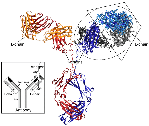
Figure 1: Overall ribbon representation of a complete AB structure. The two pairs of heavy chains are depicted in red and blue, and the corresponding light chains in yellow and grey. The dashed ellipse highlights one of the branches that bind to the antigen (the so called Fab, after fragment binding antigen), in an all-atom representation; the trapezoidal region puts in evidence the Fab variable domains (with added hydrogens), and the dashed arc illustrates the chains’ cleavage sections for these variable domains to be detached. A simplified scheme of AB-AG binding is presented in the inset.

Not surprisingly, much effort has been devoted to the determination of those $k_{\mathrm{off}}$ values, with some of the most innovative experiments involving sensitive micromanipulation techniques like atomic force microscopy (AFM) and other force probe procedures to measure AB-AG binding forces WedemayerA01 ; HinterdorferA01 ; DammerA01 ; AllenA01 ; SulchekA01 . Some further insight into the molecular structure, interactions and unbinding pathways underlying such single molecule experiments has been gained from computer simulations using “force probe” molecular dynamics (FPMD) GrubmullerIB01 . However, the question arises of to what extent the measured unbinding force in the mechanically speeded up process of pulling out the ligand relates to the thermodynamic or kinetic parameters describing the spontaneous dissociation. The later arises in the minute time scale FooteA01 in contrast to the time scales of AFM (millisecond) and FPMD (nanosecond). There is also the matter of across which pathway is unbinding being forced.

In the absence of a pulling force, one regains the spontaneous (natural) mode of AB-AG dissociation, a thermally activated barrier-crossing along a preferential path in a multidimensional energy landscape. The contributing activated states (which determine $k_{\mathrm{off}}$) may well be described in terms of a few collective coordinates, in close analogy to other studied fragmentation processes ASolovyovIB01 ; LyalinA01 ; ISolovyovA01 . Within this context, it is reasonable to constrain the many other degrees of freedom that only contribute to the negligible fine structure of the energy landscape. This is a rational approach to probe the unbinding of a complex biological system like the AB-AG one, in order to calculate the corresponding energetic barrier and derive $k_{\mathrm{off}}$ from it.

Starting with an experimentally well studied AB-AG complex, an anti-fluorescein one (vide infra), here we describe a computational approach at molecular (atomistic) level to explore its preferential unbinding pathways by probing only a few relevant degrees of freedom. A detailed analysis of its dissociation pathway and dependence on the distance and relative orientation of the molecules in question is presented. The introduction of solvent effects is also discussed along with its implications on the results, and the dissociation rate ($k_{\mathrm{off}}$) is derived from the calculated energy barriers. Following this introduction, the selection of the AB-AG system is described in detail. Next, a brief overview of the theoretical methods adopted in this study is given, in particular the computational level, the force field and the extent to which the solvent effects have been introduced. In section IV the results are presented, compared with the available experimental data, and discussed. The last section is devoted to the conclusions.

II The Test Case

Fluorescein (Flu) is a synthetic hapten. It is extensively used in fluorescence-based kinetic measurements of off-rates ($k_{\mathrm{off}}$) VossA01 , and a valuable reference system for the understanding of important immunological issues. Anti-fluorescein AB-AG complexes are also clear-cut models in the sense that Flu is a small inert and rigid ligand (see Figure 2) and the off-rates of a number of anti-Flu complexes have been found to display an Arrhenius-like behaviour SchwesingerA01 .

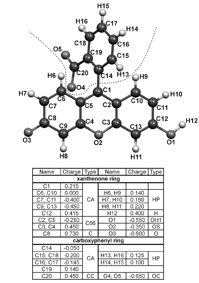
Figure 2: Structural formula and assigned atom labels for Fluorescein {2-(6- hydroxy-3-oxo-(3H)-xanthen-9yl) benzoic acid}. The force-field atom types (see sub-section III.3) and the partial charges (units of e) are listed in the table underside. The dashed line puts in evidence the two aromatic (ring) fragments labelled and grouped in the table.

The current study has been carried out for the anti-fluorescein IgG monoclonal antibody 4-4-20 (mAb4-4-20), one of the most extensively studied by thermodynamic, kinetic, structural, spectroscopic, and mutational methods (MidelfortA01 , and references within), and for which two crystallographic structures of its Fab region (highlighted in Figure 1) have already been reported HerronA01 ; WhitlowA01 . A complete IgG mAb4-4-20 molecule has two identical Fab fragments, each consisting of two constant and two variable domains. The two variable domains (labelled V_L and V_H) constitute the so called Fv fragment (also highlighted in Figure 1), which is the minimal antigen-binding fragment. In fact, there are many genetically engineered ABs that feature only the V_L and V_H domains JungA01 . This practice further endorses the idea of a system with a restricted number of binding-determinant degrees of freedom. It also makes it realistic (and computationally less demanding) to consider just the mAb 4-4-20 variable domains: V_L with 112 amino acids and V_H with 118.

III Methods

III.1 Force field

Even reducing the system to the mAb4-4-20 two variable domains plus Flu, it amounts to ca. 3600 atoms. It is, thus, too big to be computationally addressed at any level of quantum mechanics. A realistic simplification is to assume that the nuclei move in the average field created by all particles, and use an empirical fit to this field – an effective potential commonly known as a force field. One then uses the computationally less demanding classical mechanics formalism to calculate both static properties (equilibrium structures, relative energies, etc.) and the time evolution of the system.

Much effort has been devoted to develop force fields suitable for studying proteins, the CHARMM force field CHARMM22 (the one used in the present work) being one of the most widely used nowadays. Its potential energy function reads:

$$E =\sum_{i=1}^{N_{r}}k_{i}^{r}(r_{i}-r_{i}^{0})^{2}+\sum_{i=1}^{N_{\theta}}k_{i}^{\theta}(\theta_{i}-\theta_{i}^{0})^{2}$$

$$+\sum_{i=1}^{N_{\phi}}k_{i}^{\phi}\left[1+\cos(n_{i}\phi_{i}+\delta_{i})\right]$$ (1)

$$+\sum_{i=1}^{N_{\chi}}k_{i}^{\chi}(\chi_{i}-\chi_{i}^{0})^{2}+\sum_{i=1}^{N_{S}}k_{i}^{S}(S_{i}-S_{i}^{0})^{2}$$

$$+\sum_{\genfrac{}{}{0.0pt}{}{{i,j=1}}{{i<j}}}^{N}\epsilon_{ij}\left[\left(\frac{R_{ij}}{r_{ij}}\right)^{12}-2\left(\frac{R_{ij}}{r_{ij}}\right)^{6}\right]$$

$$+\sum_{\genfrac{}{}{0.0pt}{}{{i,j=1}}{{i<j}}}^{N}\frac{q_{i}q_{j}}{\varepsilon r_{ij}}.$$

The energy $E$ is a function of the positions of all atoms in the system. The first four summations are known as bonding terms: they extend to the topologically defined $N_{r}$ covalent bonds ‘$r$’, $N_{\theta}$ bond angles ‘$\theta$’, $N_{\phi}$ dihedral angles ‘$\phi$’ and $N_{\chi}$ improper torsion angles ‘$\chi$’, respectively. For some specific bond angles, an additional bonding term may be required as a function of the distance ‘$S$’ between the first and third atoms CHARMM22 . The term for the bonds describes the energy required to deform a bond from its equilibrium value (denoted by the subscript ‘$0$’), within a harmonic approximation, and an analogous description holds for the remaining harmonic terms; the dihedral term is chosen differently to satisfy the dihedral periodicity. The last two summations of equation (1) are extended to all $N$ non-bonding atom pairs $ij$ separated by three or more covalent bonds. The Lennard-Jones 6-12 potential term accounts for the van der Waals (vdW) interactions: for each atom type (say $i$), there is a $R_{i}$ distance corresponding to a well depth $\epsilon_{i}$, with $R_{i}=2^{1/6}\sigma_{i}$ and $\sigma_{i}$ the distance for which the Lennard-Jones potential equals zero; the Lennard-Jones parameters between pairs of different atoms are obtained from combination rules, the $\epsilon_{ij}$ values based on the geometric mean of $\epsilon_{i}$ and $\epsilon_{j}$ and $R_{ij}$ values form the arithmetic mean between $R_{i}$ and $R_{j}$. The Coulombic potential is defined for the pairs of charges $q_{i}$ and $q_{j}$ separated by a distance $r_{ij}$, and for a given dielectric constant $\varepsilon$ (the vacuum one by default). The equilibrium values in the harmonic terms and the $R_{i}$ and $\epsilon_{i}$ values are parameters derived from experimental data (e.g., crystallographic structures) and ab initio quantum mechanical calculations on small reference molecules, presented and discussed in ref. CHARMM22 . Partial charges ($q_{i}$, $q_{j}$) are also derived from such ab initio calculations.

III.2 Implicit solvent

Proteins operate in aqueous solution. Solvation, stability and dissociation of molecules in water are largely governed by electrostatic interactions. This is particularly pertinent in proteins: more than 20% of all amino acids in globular proteins are ionized under physiological conditions and polar side-chains occur in over another 25% amino acids FogolariA01 . However, introducing explicit water molecules in a computational simulation to account for solvent effects dramatically increases the calculation time. Moreover, when the calculations involve any energy minimisation-based technique like calculating minimum energy reaction paths, the explicit water molecules will arrange in a single conformation matrix, exerting forces on the solute that are very different from the solvent mean force.

Alternatively, a continuum treatment of the solvent as a uniform dielectric may provide an accurate enough description of such interactions, as long as one accounts for the fact that a protein in aqueous solution (the physiological medium) yields a system with two very different dielectric media FogolariA02 . A most physically correct implicit solvent model arises from solving the so-called Poisson–Boltzmann (PB) equation (see FogolariA02 ; BakerA01 , and references within). The protein (macromolecule) is treated as a low-dielectric cavity bounded by the molecular surface and containing partial atomic charges – typically taken from the classical molecular mechanics force field. The solvent (water) is implicitly introduced by assuming a high-dielectric surrounding of the protein. And since under physiological conditions macromolecules are dissolved in dilute saline solutions (water with a dissolved electrolyte), a term for the average charge density due to the mobile ions is also included. This classical continuum electrostatics treatment relies on the (reasonable) assumption that it is possible to replace the ionic potential of mean force with the mean electrostatic potential, neglecting non-Coulombic interactions (e.g., vdW) and ion correlations. The actual PB equation reads:

$$\nabla\cdot[\varepsilon(\mathbf{r})\nabla\varphi(\mathbf{r})] =-4\pi\rho(\mathbf{r})$$ (2)

$$-4\pi\sum_{i=1}^{N}e\mathrm{q}_{i}n_{i}(\mathbf{r})\lambda(\mathbf{r}),$$

with

$$n_{i}(\mathbf{r})=n_{i}^{0}\exp(e\mathrm{q}_{i}\varphi(\mathbf{r})/k_{\mathrm{B}}\mathrm{T}).$$ (3)

Equation (2) relates the electrostatic potential $\varphi$ to the distribution of the protein atomic partial charges (charge density $\rho$), the dielectric properties of both the protein and solvent ($\varepsilon$, position dependent $(\mathbf{r})$), and the charge density due to the mobile ions given by the summation term; $q_{i}$ is the charge of ion type $i$, $n_{i}(\mathbf{r})$ its local concentration, $e$ the elementary charge and $\lambda(\mathbf{r})$ a parameter that describes the ions’ accessibility at position $\mathbf{r}$. The boundary condition is $\varphi(\mathbf{\infty})=0$. For each ion type, $n_{i}(\mathbf{r})$ is described by a Boltzmann distribution (3) where $n_{i}^{0}$ is the ion’s concentration in bulk solution, $k_{B}$ the Boltzmann constant and T the absolute temperature. As for the accessibility parameter, a general consensus is that any point within one ionic radius from the macromolecule is inaccessible (i.e., $\lambda(\mathbf{r})=0$), and it is implicit that the region inside the macromolecular surface is inaccessible. The remaining region outside has $\lambda(\mathbf{r})=1$. A typical value for the ionic raidus is the one of Cl^- (2 Å), considering that Na⁺Cl^- (sodium chloride) is a most frequently chosen electrolyte.

A description of the several possible approximations and numerical techniques used to solve equation (2) is beyond the scope of the present paper, the reader being referred to the supporting literature of the software used in this work, APBS (Adaptative Poisson–Boltzmann Solver) BakerA01 ; SinghA01 . Briefly, the solute’s charges are mapped onto a mesh and the electrostatic potential in the presence of the dielectric continuum solvent is determined at each point, via a finite difference numerical solution of the PB equation. The mesh being a finite one, it is necessary to set up the boundary potentials (at the lattice edge) accordingly. For the present work, they are approximated by the sum of the Debye–Hückel potentials of all the charges, meaning

$$\varphi=\sum_{i=1}^{N}e\mathrm{q}_{i}\frac{\exp(-r_{i}/\lambda_{D})}{\varepsilon_{\mathrm{water}}r_{i}},$$ (4)

where $\lambda_{D}$, the Debye length, reads

$$\lambda_{D}=\sqrt{\frac{\varepsilon_{\mathrm{water}}k_{\mathrm{B}}\mathrm{T}}{4\pi N_{A}\sum_{i=1}^{N}n_{i}^{0}e^{2}q_{i}^{2}}}.$$ (5)

III.3 Fluorescein parameters

The available CHARMM parameterisation already has parameters for all amino acids but not for fluorescein, so one has first to describe the later consistently with the force field. In the present work, the required bonding and Lennard-Jones parameters where derived by analogy to similar ones existing in CHARMM. Partial atomic charges were fitted to reproduce the molecular electrostatic potential (MEP) at selected points around the molecule according to the Merz–Singh–Kollman scheme SinghA02 ; BeslerA01 implemented in the Gaussian03 program Gaussian03 . The points are located in layers around the molecule, the first layer corresponding to the van der Waals molecular surface scaled by a factor of 1.4; the default scheme then adds three more layers with scaling factors 1.6, 1.8 and 2.0. The MEP was generated at the DFT/B3LYP level with the 6-31G(d) basis set. DFT (density functional theory) is now a widely used and computationally convenient quantum mechanical method well documented in many reference books (e.g., ParrB01 ): it makes use of exchange correlation functionals dependent on the electron density and its gradient to tackle electron correlation effects. B3LYP was the functional of choice and stands for the three-parameter Becke functional combined with the Lee-Yang-Parr correlation functional ParrB01 .

For the quantum mechanical calculations, the coordinates for the starting Flu conformation were taken from the complex crystal structure with the best resolution (1.85 Å WhitlowA01 ), which has the coordinates deposited in the RCSB Protein Data Bank BermanA01 with entry name 1FLR. Only the acidic deprotonated form of Flu was considered, since this is the active form in the experiments underlying the current study. The structure was energy optimized before charge fitting. The charges were then further refined by similarity to the set of already defined ones in the CHARMM force field (for details on the approach see PaciA01 ; HenriquesA01 ; HenriquesA02 ). The ensuing Flu set of parameters was then used as an extension of the CHARMM parameterisation, the corresponding CHARMM atom types and partial charges being indicated in Figure 2.

III.4 Reference geometry

The variable domains (V_L and V_H) were extracted from the L and H segments of the anti-Flu 4-4-20Fab 1FLR crystal structure WhitlowA01 ; BermanA01 . Crystallographic waters were stripped from the structure and the C-terminal amino acids were capped with –NH₂ functional groups. A representation of the system is shown in Figure 3. The positions of the protein’s missing hydrogens were initially guessed. Next, any latent close contacts or anomalous bonding positions were cleared out by relaxing the structure to an energy gradient tolerance of 0.05 eV$\cdot$Å^-1, at the classical mechanics level using the NAMD program NAMD with the extended CHARMM parameterisation. This relaxed structure fully retains the experimental X-ray conformational features and it was used as the starting conformation for the scanning. A full structure optimisation (i.e., using a tighter energy gradient tolerance) was also carried out but it introduced many small errors at the protein’s secondary structure level. This is because secondary structure relies on a network of backbone hydrogen bonds, which are less accurately described in the framework of the simplified molecular mechanics force field theories. The CHARMM energy difference between the relaxed and fully minimised geometries is $\sim$100 eV. The crystallographic structure itself has been resolved at a temperature of $\sim$290 K WhitlowA01 , thus an estimate of the corresponding average thermal energy (considering $k_{B}T$ per degree of freedom) amounts to $\sim$270 eV for our simulation system. This indicates that the full minimisation is only reaching some local minima. Considering the above referred limitations of the force field, it is judicious to take the minimally relaxed structure (closer to the X-ray one) as the reference structure for the subsequent simulations.

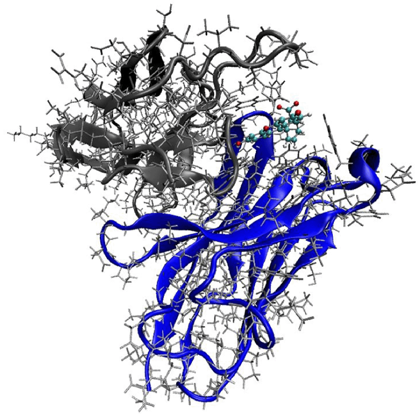
Figure 3: All-atom representation of the Fv-fragment of the mAb4-4-20-Flu complex structure. The ribbon representation highlights the backbone of the two chains, the H-chain in blue and the L-chain in gray. The Flu molecule is depicted in ball-and-stick and coloured by element (CPK space-filling).

Flu is a particularly rigid molecule. Its essential degree of freedom is the torsion around the bond between the xanthenone and the carboxyphenyl aromatic rings (see Figure 2), defining the angle between the planes of these two rings. This angle has the value of $-$63^∘ in both the crystal complexed form WhitlowA01 and the crystalline free Flu DuBostA01 . For the above referred CHARMM energy relaxed structure, the value of this angle is $-$67^∘. An energy optimization was also carried out for the hapten alone (without the AB), the value for the angle in question being -62^∘. Moreover, the RMSD (root-mean-square deviation) between the crystallographic and relaxed Flu bound structures is 0.201 Å. These results are a good indication of the validity of the derived set of CHARMM parameters.

III.5 Distance scanning

In the pursuit for the suitable reaction coordinates to describe the system’s unbinding, the distance between the protein and Flu mass-centres could be a first option, in close analogy to some cluster fission processes ASolovyovIB01 . Yet for reasons that will become clear next, a distance between two rationally selected atoms has been considered instead.

The shape of the binding pocket hosting Flu is most complementary to this hapten, with a few amino acids at the rim of the pocket gating the entrance. Superimposing the two available crystal structures results in an overall RMSD of 0.419 Å for the Flu atoms and 1.854 Å for the protein, with a few of those rim amino acids exhibiting some of the larger individual RMSD values (up to 3.7 Å). Out of those, five amino acids – His31_L, Asn33_L, Tyr56_H, Tyr102_H and Tyr103_H – strategically “frame” amino acid Arg39_L at the bottom of the pocket, as depicted in Figure 4. Amino acids are labelled

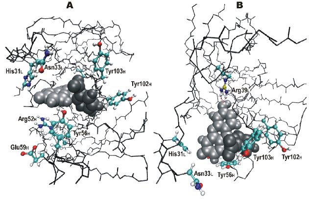
Figure 4: Fluorescein (van der Waals spheres in shades of grey) docked in the antibody’s binding cavity. The backbone of the antibody is depicted in black sticks; the framing amino acid acids (labelled as described in the text) have their side-chains displayed in coloured ball-and-stick. (A) front view of the entrance of the cavity. (B) top view showing residue Arg39_L at the bottom of the cavity, with its atom C_ζ (zeta-carbon, standard nomenclature) highlighted in yellow: the red dotted lines represent hydrogen bonding between Arg39_L and the hapten.

(in the text and Figure 4) according to the standard amino acid 3-letter code (LehningerB01 ; see also http://www.chem.qmul.ac.uk/iupac/ AminoAcid/), the number of the amino acid in the 1FLR file and the chain identifier in subscript (e.g., Arg39_L, refers to an Arginine that is numbered 39 in the L-chain). As highlighted in Figure 4-B, Arg39_L has its +1-ionized group (centred on atom C_ζ) directly involved in hydrogen bonding to the hydroxyl group of Flu (atoms O1–H12 in Figure 2). Arg39_L is also a mutation introduced during the maturation process of mAb4-4-20 JimenezA01 : the original residue was a neutral, weakly polar Histidine. Upon this His-to-Arg mutation a slowing in the unbinding of Flu by a 1.5-fold was experimentally observed JimenezA01 , no doubt in consequence of the increased attraction between the mutated amino acid 39_L and Flu. Thus, it was only logical to consider the distance between the groups of Arg39_L and Flu engaged in that driving hydrogen bonding as a most likely unbinding coordinate.

The distance between the C_ζ atom of Arg39_L and the Flu’s hydroxyl oxygen (O1) was then set as the appropriate coordinate for scanning. The scanning started from the distance in the reference conformation and progressed in increments of 0.25 Å until a $\sim$40 Å distance. At this distance and for the set cut-off, the interaction energy between the hapten and the AB becomes zero. The scanning was also performed for a few decreasing steps, i.e., for distances smaller than the one in the reference structure. The distance value at each scanning step was imposed by means of a strong harmonic constraint (force constant = 26 eV$\cdot$Å^-2) between the referred oxygen and a dummy atom placed at the same coordinates of the C_ζ atom. The need for a dummy atom arises from the fact that, in CHARMM, the non-bonding energy of all atom pairs separated by less than three covalent bonds is excluded CHARMM22 ; the introduced harmonic constraint is an “artificial bond” and therefore should not be directly set between the C_ζ and OH atoms, otherwise several pair interactions between Arg39_L and Flu would be wrongly excluded.

For each scanning step, the system was energy minimised with NAMD to an energy gradient tolerance $\leq$ 4$\times$10^-4 eV$\cdot$Å^-1. A 12 Å cut-off on long-range interactions with a switch smoothing function between 10 and 12 Å was used. During minimisation, the hapten was free to move (subject only to the scanning harmonic constraint) while the AB was kept frozen for all but the side-chain atoms of a few key amino acids gating the passage of the hapten. The unconstrained side-chains belong to His31_L, Asn33_L, Arg52_H, Tyr56_H, Glu59_H, Tyr102_H and Tyr103_H. The reported energy of each minimised structure was calculated after removing the referred harmonic constraint. In NAMD, it is not possible to set two different dielectrics within the same system, so minimisations were performed for $\varepsilon$ = 1, and solvent effects were introduced as corrections a posteriori, as described next.

For the final conformation of each scanning step, the electrostatic energy was recalculated using the APBS program (refer to sub-section III.2). The conformation of the last scanning step roughly occupies a 70 Å-side cubic box. The side was extended by an extra 20 Å for solvent media, resulting in a 90$\times$90$\times$90 ų box that was set equal for all scanning steps. Calculations were performed using the APBS’ adaptive refinement HolstA01 . A low dielectric constant of $\epsilon$ = 2 was set for the macromolecule cavity FogolariA02 ; PetersenA01 and the typical water value of $\epsilon\approx 80$ was set for the continuum solvent medium. The effect of a dilute electrolyte in solution was assessed with a second run of calculations, for a salt bulk concentration of 0.150 mol$\cdot$dm^-3 as in a typical physiological media SinghA02 , and a temperature of 298 K.

III.6 Exploring relative orientations

The distance scanning scheme above described does not enforce an escaping channel along a straight line, nor does it restrain the AB-hapten relative orientations. For the sake of completion, a comprehensive overlook of the two molecules relative position and mutual orientation should be performed. The designated appropriate descriptors are the spherical coordinates ($r$, $\theta$, $\phi$) and three Euler angles ($\alpha$, $\beta$, $\gamma$), for which two coordinate frames are required. The referential frame, set as the protein’s principal axes of moment of inertia given that the protein is fixed in space, and the moving-body local frame, i.e. the Flu frame. Care was taken to select this later, considering that during the scanning Flu does not evolve in space as a completely rigid body. Its centre was set in Flu’s atom C1 since along the scanning the position of Flu’s mass centre is approximately coincident to this atom (0.2-0.4 Å RMSD). The $xy$ plane was made coincident to the rigid xanthenone ring, with the $x$ axis pointing in the direction of atom O1, as displayed in Figure 5.

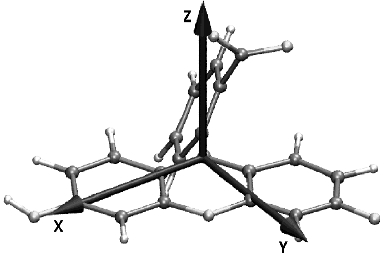
Figure 5: System of internal axes for Flu.

III.7 Calculation of $k_{\mathrm{off}}$

In compliance with the experimentally reported Arrhenius-like behaviour SchwesingerA01 and within the context of the reaction-rate theory HanggiA01 , the off-rate constant along the scanned pathway was computed using the expression,

$$k_{\mathrm{off}}=\omega\exp(-\Delta E^{{\ddagger}}/k_{\mathrm{B}}\mathrm{T})$$ (6)

where $\omega$ is the pre-exponential factor determining how frequently the system approaches the barrier, and $\Delta E^{{\ddagger}}$ is the activation energy (i.e., the barrier height). The harmonic approximation was used to estimate the Arrhenius-like pre-factor. It reads

$$\omega=\frac{1}{2\pi}\sqrt{k/\mu},$$ (7)

where $\mu$ is the reduced mass of the system and $k$ the harmonic force constant. This latter was obtained from parabolic fit of the data (the bounding region of the well in the energy profiles) using the Mathematica® software package. For systems similar to the one presented here (with reduced masses in the 200-500 range and binding pocket’s length within 3-7 Å), an estimation of the frequency $\omega$ falls in the $10^{11}$-$10^{12}$ s^-1 range.

IV Results and Discussion

IV.1 Energetic and structural analysis

The energy profiles resulting from the scanning runs with and without solvent correction are plotted in Figures 6 and 7.

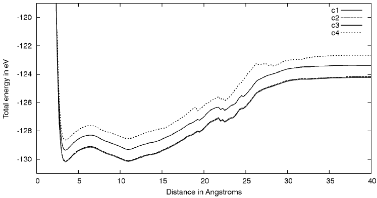
Figure 6: Energy profiles (in vacuo) for different distance scanning runs, corresponding to different constraining schemes on the protein atoms. Each curve corresponds to a different number of gating amino acid side-chains that were allowed to move during each scanning, namely seven side chains (c1), six (c2) five (c3) and four (c4) (details in the text).

Figure 6 displays the in vacuo results for four different scanning runs, corresponding to different constraining schemes on the protein atoms. The scheme referring to the seven unconstrained side-chains enumerated in sub-section III.5 has been labelled ‘c1’ in Figure 6. To better assess on the influence of those 7 amino acids on the escaping profile, they were subject to successive constraining procedures, exemplified in Figure 6 for three representative cases, labelled ‘c2’, ‘c3’ and ‘c4’, that correspond to six, five and four unconstrained side chains (out of the initial seven). The plotted ‘c3’ curve, for instance, results from moving only the side-chains of the 5 gating residues sginaled out in the second paragraph of sub-section III.5 and visible in Figure 4-B.

The constraining limit is the set of amino acids Asn33_L, Tyr56_H, Tyr102_H and Tyr103_H corresponding to the ‘c4’ curve. Within this limit, no general significant differences on the energy profile arise from the explored different schemes. These 4 amino acids always experience significant conformational changes upon the hapten’s passage, in comparison to the remaining moving ones which just slightly adjust positioning. The plane defined by the side-chain oxygens of the 4 amino acids in question can be taken as the outmost limit of the protein’s pocket, and it is intersected at a $\sim$15 Å scanning distance. Below this separation distance, the total energy plots in Figure 6 depict the expected profile for an activated process. For the different curves, the height and shape of the energetic barrier at $\sim$7 Å is essentially the same: 1.029, 1.027, 1.060 and 1.026 eV respectively for 7, 6, 5 and 4 moving side-chains. Past the 15 Å distance, the in vacuo profiles depict an asymptotic increase to a final plateau above the referred energetic barrier, making unbinding unfeasible. Predictably, the inclusion of solvent effects rectify the asymptotic behaviour depicted in the in vacuo profiles, as exemplified in Figure 7 for two scanning runs.

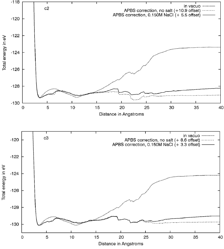
Figure 7: Comparison of the distance scanning energy profiles in vacuo and with implicit solvent corrections (with and without dissolved electrolyte), for the ‘c2’ and ‘c3’ constraining schemes.

At larger separation distances the energy profile has been significantly flattened, ant it is also for the larger distances that the effect of the dissolved electrolyte becomes perceptible. In solution, the electrostatic interactions between the protein and the escaping hapten are effectively screened by the high-dielectric, allowing for unbinding to happen. Of relevance is also the decrease in the height of the energetic barrier at  $\sim$7 Å: with implicit solvent effects, this barrier value is 0.863 and 0.871 eV, respectively for the ‘c2’ and ‘c3’ schemes.

The jagged contour emerging at $\sim$20 Å also deserves some attention. A detailed analysis of the energetic components was carried out, with particular emphasis on the Coulombic component, as exemplified in Figure 8 for scanning run ‘c2’.

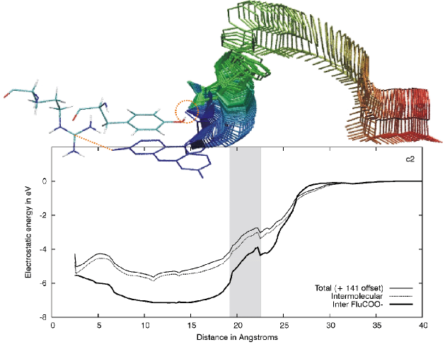
Figure 8: Electrostatic energy profiles (in vacuo) for the overall system, its intermolecular component and the interaction energy between the protein and the COO^- group (atoms C20, O4, O5 of the Flu’s carboxyphenyl ring; see Figure 2). The picture on top portraits the path of that ring along the scanning: the dashed yellow straight line puts in evidence the coordinate being scanned while the circle emphasises the anchor point of the COO^- group at the protein’ surface (see details in the text). The grey area puts in evidence a jagged region in the profile.

A previous work had already shown that, at larger distances, electrostatics play a major role in fragmentation ISolovyovA01 . By comparing Figures 7 and 8, one perceives the jagged pattern similarities between the total energy and its electrostatic component. Moreover, the electrostatic energy and its intermolecular component – i.e., the electrostatic interaction energy between the protein and the hapten – run parallel. To this intermolecular energy, a major contribution comes from the COO^- group of Flu. This group gets anchored via hydrogen-bonds at the protein’s surface as the hapten leaves the pocket: the anchor point is yellow circled in the top picture of Figure 8. The hapten rotates around this point as the scanning distance is further increased, until it finally detaches from the surface. The detachment features a somewhat irregular trajectory of the escaping hapten: it is the region of the top picture in Figure 8, right above the grey area highlighting the jagged contour in the plot. A better perception of the hapten’s rotation as it leaves the binding pocket can be gained from the plotting of the Euler angles along the scanning, presented in Figure 9. The steeper variation of the angles in the 15-20 Å region corresponds to the anchoring track of the COO^- group at the protein’ surface. As the hapten detaches, a swift change in its orientation is observed, made evident by the plots for the Euler angles from $\sim$20 Å on. At this stage, one can not ascertain whether or not this pronounced “trapping” of the hapten to the protein’ surface is a genuine feature of the unbinding. That would at least require the other known mutations of the anti-fluorescein mAb4-4-20 to be subject to an analogous study, which is beyond the scope of the present paper.

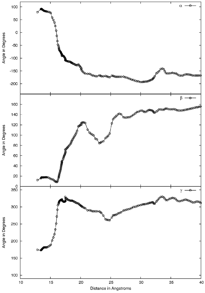
Figure 9: Euler angles as a function of the scanned distance coordinate.

The fact remains that, on the overall, the total energy profiles are smooth (without discontinuities), as clear from the top plot in Figure 10 of the energy as a function of both the scanning coordinate and the radial distance ($r$). They portray a plausible unbinding channel, provided solvent effects are included, though one can not claim that they correspond to the minimum energy pathway. One possible step to assess that would be to perform a more comprehensive probing of the positional/orientational space of the hapten – beyond the points determined by the presently selected reaction coordinate. Yet, such a study involves a substantial computational effort, even if confined to some plausible escaping window in space. On the other hand, the presently computed profiles can be used to derive $k_{\mathrm{off}}$, and by comparison to the corresponding experimental values(s), a first evaluation of the scanning approach here introduced can be made.

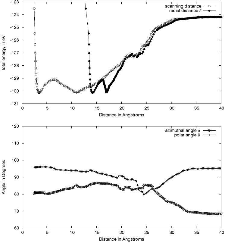
Figure 10: Spherical coordinates along the ‘c2’ scanning run. The total energy of the system is plotted as a function of both the radial distance ($r$) and the scanned distance coordinate. The angles $\theta$ and $\phi$ are plotted only as a function of the scanning distance coordinate.

IV.2 $k_{\mathrm{off}}$ determination

Table I presents the calculated values of $k_{\mathrm{off}}$, with and without solvent correction, resulting from parabolic fit to the profiles (0.99 $\leq$ R² $\geq$ 0.87), considering the energy barrier at $\sim$7 Å (vide supra). Experimentally available $k_{\mathrm{off}}$ values are also presented for comparison. It becomes immediately evident that, even for an extensively studied system like the mAb4-4-20–fluorescein one, experimental $k_{\mathrm{off}}$ values may differ by an order of magnitude, depending on setup conditions and techniques JimenezA01 ; MummertA01 ; BoderA01 . As for our estimated values, while the in vacuo results are off-range, the solvent-corrected ones are comparable to the experimental results. The equilibrium distance between the antibody and the hapten (the well minimum) also compares better to the experimental value in the case of the solvent-corrected simulations. Finally, remark that the different constraining schemes have little influence on the order of magnitude of the $k_{\mathrm{off}}$ values.

Table 1: Kinetic and equilibrium parameters obtained from calculations based on the computational scanning. Available experimental values are also presented for comparison: (a) and (c) determined in solution (ref. MummertA01 and BoderA01 respectively), and (b) at a surface by SPR JimenezA01 .

parameter	simulations				experimental	T(K)
	in vacuo		solvent corrected
	c2	c3	c2	c3
					$1.9\times 10^{-3}$ (a)	291
$k_{\mathrm{off}}$(s-1)	$3.4\times 10^{-6}$	$6.8\times 10^{-6}$	$4.1\times 10^{-3}$	$5.4\times 10^{-3}$	$6.8\times 10^{-3}$ (b)	298
					$4.3\times 10^{-3}$ – $2.5\times 10^{-2}$ (c)	298
equilibrium	3.50	3.55	3.60	3.65	3.65	291
distance (Å)

V Concluding Remarks

Here we presented our first attempt to describe the unbinding of a complex biomolecular system in terms of a reduced set of relevant generalized coordinates while restricting most of its conformational internal degrees of freedom. The reported results open a practical and physically sound procedure to compute energy profiles along the selected reaction coordinate(s). This was demonstrated in the present work for an experimentally well studied complex of the biologically relevant antigen-antibody system. For the example in question, it was actually possible to find a distance dependent escaping channel in the multidimensional potential energy landscape, thus reducing the unbinding to a low-dimensional problem: the system seems to be efficiently bound by this one distance coordinate. The effect of the solvent was also accounted for, and despite the fact that it was introduced as a correction a posteriori, it allowed us to ascertain that this is one effect that needs to be included, for it has a significant influence in the overall energetic profile and subsequent parameters derived from it. With solvent effects, the derived off-rates are in reasonable agreement with the experimentally determined ones, a result that can be regarded as an indicator that ours is indeed a realistic approach.

The proposed approach would no doubt benefit from further refinements, namely in the way solvent effects are introduced (viz. include them during scanning, both implicit and explicitly) and in the kinetic model, which we intend to carry on in the near future. We also have in mind to apply this same approach to the maturation series and engineered mutants of the 4-4-20–fluorescein complex. That would allow us to further test our strategy, in particular its sensitiveness to the energetic differences arising from antibody’s single-point mutations. In addition, computed association rates would be valuable parameters in different areas of immunological research, namely theoretical immunology HermannA01 . Remark also that calculated $k_{\mathrm{off}}$ values could be used to determine the related association rate $k_{\mathrm{on}}$ using the relation $k_{\mathrm{on}}=$ $k_{\mathrm{off}}/K_{\mathrm{d}}$JimenezA01 , for those systems where only the equilibrium dissociation constant $K_{d}$ has been experimentally measured. And by identifying and rationalize the involved key structural features and interactions determining the unbinding, one could make insightful predictions and propose, for instance, affinity-enhancing mutations. Our long term goal is to extend our research to other molecular recognition processes besides the antigen-antibody one and to test the applicability and universality of our approach.

- [1] A. V. Solov’yov, J.-P. Connerade, and W. Greiner. Latest Advances in Atomic Cluster Collisions. Imperial College Press, London, 2004.
- [2] A. Lyalin, O. I. Obolensky, A. V. Solov’yov, and W. Greiner. Int. J. Modern Phys. E, 15:153–195, 2006.
- [3] I. A. Solov’yov, A. V. Yakubovich, A. V. Solov’yov, and W. Greiner. J. Exp. Theo. Phys., 103:463–471, 2006.
- [4] G. J. Wedemayer, P. A. Patten, L. H. Wang, P. G. Schultz, and R. C. Stevens. Science, 276:1665–1669, 1997.
- [5] David L. Nelson and Michael M. Cox. Lehninger Principles of Biochemistry. W.H. Freeman and Company, New York, 2005.
- [6] Tim Manser. Textbook germinal centers? The Journal of Immunology, 172:3369–3375, 2004.
- [7] F. Schwesinger, R. Ros, T. Strunz, D. Anselmetti, H.-J. G ntherodt, A. Honegger, L. Jermutus, L. Tiefenauer, and A. Plückthun. Proc. Natl. Acad. Sci. U.S.A., 97:9967–9971, 2000.
- [8] J. Foote and H. N. Eisen. Proc. Natl. Acad. Sci. U.S.A., 92:1254–1256, 1995.
- [9] R. Jimenez, G. Salazar, T. Joo J. Yin, and F. E. Romesberg. Proc. Natl. Acad. Sci. U.S.A., 101:3803–3808, 2004.
- [10] P. Hinterdorfer, W. Baumgartner, H. J. Gruber, K. Schlicher, and H. Schindler. Proc. Natl. Acad. Sci. U.S.A., 93:3477–3481, 1996.
- [11] U. Dammer, M. Hegner, D. Anselmetti, P. Wagner, M. Dreier, W. Huber, and H.-J. Güntherodt. Biophys. J., 70:2437–2441, 1996.
- [12] S. Allen, X. Chen, J. Davies, M. Davies, A. C. Dawkes, J. C. Edwards, C. J. Roberts, J. Sefton, S. J. B. Tendler, and P. M. Williams. Biochemistry, 36:7457–7463, 1997.
- [13] T. A. Sulchek, R. W. Friddle, E. Y. Lau K. Langry, H. Albrecht, T. V. Ratto, S. J. DeNardo, M. E. Colvin, and A. Noy. Proc. Natl. Acad. Sci. U.S.A., 102:16638–16643, 2005.
- [14] H. Grubmüller. Protein-Ligand Interactions, chapter Force probe molecular dynamics simulations, pages 493–515. The Human Press Inc., NJ USA, 2005.
- [15] E. W. Voss Jr. J. Mol. Recognit., 6:51–58, 1993.
- [16] K. S. Midelfort, H. H. Hernandez, S. M. Lippow, B. Tidor, C. L. Drennan, and K. D. Wittrup. J. Mol. Biol., 343:685–701, 2004.
- [17] J. N. Herron, X. M. He, M. L. Mason, E W. Voss Jr., and A. B. Edmundson. Proteins, 5:271–280, 1989.
- [18] M. Whitlow, A. J. Howard, J. F. Wood, E. W. Voss Jr., and K. D. Hardman. Protein Eng., 8:749–761, 1995.
- [19] S. Jung and A. Pluckthun. Protein Eng., 10:959–966, 1997.
- [20] A. D. MacKerell Jr., D. Bashford, M. Bellott, R. L. Dunbrack Jr., J. Evanseck, M. J. Field, S. Fischer, J. Gao, H. Guo, S. Ha, D. Joseph, L. Kuchnir, K. Kuczera, F. T. K. Lau, C. Mattos, S. Michnick, T. Ngo, D. T. Nguyen, B. Prodhom, W. E. Reiher III, B. Roux, M. Schlenkrich, J. Smith, R. Stote, J. Straub, M. Watanabe, J. Wiorkiewicz-Kuczera, D. Yin, and M. Karplus. J. Phys. Chem. B, 102:3586–3616, 1998.
- [21] F. Fogolari, A. Brigo, and H. Molinari. J. Mol. Recognit., 15:377–392, 2002.
- [22] F. Fogolari, P. Zuccato, G. Esposito, and P. Viglino. Biophys. J., 76:1–16, 1999.
- [23] N. A. Baker, D. Sept, Joseph S., M. J. Holst, and J. A. MacCammon. Proc. Natl. Acad. Sci. U.S.A., 98:10037–10041, 2001.
- [24] U. C. Singh and P. A. Kollman. J. Comput. Chem., 5:129–145, 1984.
- [25] B. P. Singh, H. B. Bohidar, and S. Chopra. Biopolymers, 31:1387–1396, 1991.
- [26] B. H. Besler, K. M. Merz Jr., and P. A. Kollman. J. Comput. Chem., 11:431–439, 1990.
- [27] Gaussian 03: Revision C.02, M. J. Frisch, G. W. Trucks, H. B. Schlegel, G. E. Scuseria, M. A. Robb, J. R. Cheeseman, J. A. Montgomery Jr., T. Vreven, K. N. Kudin, J. C. Burant, J. M. Millam, S. S. Iyengar, J. Tomasi, V. Barone, B. Mennucci, M. Cossi, G. Scalmani, N. Rega, G. A. Petersson, H. Nakatsuji, M. Hada, M. Ehara, K. Toyota, R. Fukuda, J. Hasegawa, M. Ishida, T. Nakajima, Y. Honda, O. Kitao, H. Nakai, M. Klene, X. Li, J. E. Knox, H. P. Hratchian, J. B. Cross, C. Adamo, J. Jaramillo, R. Gomperts, R. E. Stratmann, O. Yazyev, A. J. Austin, R. Cammi, C. Pomelli, J. W. Ochterski, P. Y. Ayala, K. Morokuma, G. A. Voth, P. Salvador, J. J. Dannenberg, V. G. Zakrzewski, S. Dapprich, A. D. Daniels, M. C. Strain, O. Farkas, D. K. Malick, A. D. Rabuck, K. Raghavachari, J. B. Foresman, J. V. Ortiz, Q. Cui, A. G. Baboul, S. Clifford, J. Cioslowski, B. B. Stefanov, G. Liu, A. Liashenko, P. Piskorz, I. Komaromi, R. L. Martin, D. J. Fox, T. Keith, M. A. Al-Laham, C. Y. Peng, A. Nanayakkara, M. Challacombe, P. M. W. Gill, B. Johnson, W. Chen, M. W. Wong, C. Gonzalez, and J. A. Pople. Gaussian Inc., Wallingford CT, 2004.
- [28] R. G. Parr and W. Yang. Density-Functional Theory of Atoms and Molecules. Oxford University Press, New York, 1994.
- [29] H. Berman, K. Henrick, H. Nakamura, and J. L. Markley. Nucleic Acids Research: Database issue D1-D3 doi:10.1093/nar/gkl971, 00, 2006.
- [30] E. Paci, A. Caflisch, A. Plückthun, and M. Karplus. J. Mol. Biol., 314:589–605, 2001.
- [31] E. S. Henriques, M. Bastos, C. F. G. C. Geraldes, and M. J. Ramos. Int. J. Quant. Chem., 73:237–248, 1999.
- [32] E. S. Henriques, M. A. C. Nascimento, and M. J. Ramos. Int. J. Quant. Chem., 106:2107–2121, 2006.
- [33] L. Kale, R. Skeel, M. Bhandarkar, R. Brunner, A. Gursoy, N. Krawetz, J. Phillips, A. Shinozaki, K. Varadarajan, and K. Schulten. J. Comp. Phys., 151:283–312, 1999.
- [34] J. P. DuBost, J. M. Leger, J. C. Colleter, P. Levillain, and D. Fompeydie. C. R. Acad. Sci. Paris Sér. II, 292:965–968, 1981.
- [35] M. J. Holst, N. A. Baker, and F. Wang. J. Comput. Chem., 21:1343–1352, 2000.
- [36] M. T. Neves-Petersen and S. B. Petersen. Biotechnology Ann. Rev., 9:315–394, 2003.
- [37] P. Hänggi, P. Talkner, and M. Borkovec. Rev. Mod. Phys., 62:251–341, 1990.
- [38] M. E. Mummert and E. W. Voss Jr. Biochemistry, 35:8187–8192, 1996.
- [39] E. T. Boder, K. S. Midelfort, and K. D. Wittrup. Proc. Natl. Acad. Sci. U.S.A., 97:10701–10705, 2000.
- [40] M. E. Meyer-Hermann, P. K. Maini, and D. Iber. Math. Med. Biol., 23:255–277, 2006.