Confining ensemble of dyons
Abstract
We construct the integration measure over the moduli space of an arbitrary number of kinds of dyons of the pure gauge theory at finite temperatures. The ensemble of dyons governed by the measure is mathematically described by a (supersymmetric) quantum field theory that is exactly solvable and is remarkable for a number of striking features: 1) The free energy has the minimum corresponding to the zero average Polyakov line, as expected in the confining phase; 2) The correlation function of two Polyakov lines exhibits a linear potential between static quarks in any -ality non-zero representation, with a calculable string tension roughly independent of temperature; 3) The average spatial Wilson loop falls off exponentially with its area and the same string tension; 4) At a critical temperature the ensemble of dyons rearranges and de-confines; 5) The estimated ratio of the critical temperature to the square root of the string tension is in excellent agreement with the lattice data.
pacs:
11.15.-q,11.10.Wx,11.15.TkI Introduction
Isolated dyons in the pure Yang–Mills theory are (anti) self-dual solutions of the equation of motion , which in an appropriate gauge are Abelian at large distances from the centers and carry unity electric and magnetic charges with respect to the Cartan generators :
| (1) |
For the gauge group on which we focus in this paper there are Cartan generators associated with the simple roots of the group, where the is on the place, that are supplemented by the generator to make the set of dyons electric- and magnetic-neutral. The first dyons are also called the Bogomolny–Prasad–Sommerfield (BPS) monopoles BPS . The last dyon is sometimes called the Kaluza–Klein monopole: in the gauge where the first dyons are described by a static field the last has time-dependent fields inside the core. However, by a periodic time-dependent gauge transformation one can make the last one time-independent (at the cost of a time dependence inside other dyons), therefore the distinction of the last dyon is illusory and we shall treat all of them on the same footing. The cyclic symmetry of dyons is evident from the -branes point of view LeeYi ; DHKM-99 .
In this paper we explore the properties of a semiclassical vacuum built of a large number of dyons of kinds.
To make the semiclassical calculation of the Yang–Mills partition function well defined one needs i) to expand about a true saddle point of the action, ii) to be sure that the quantum fluctuation determinant is infrared-finite. For an isolated dyon the first is true but the second is false. For an arbitrary superposition of different-kind dyons the second is true but the first is wrong. To satisfy both requirements one can consider dyons as constituents of the Kraan–van Baal–Lee–Lu (KvBLL) instantons with non-trivial holonomy KvB ; LL , which are saddle points of the Yang–Mills partition function as they are exact self-dual solutions of the equations of motion. At the same time the fluctuation determinant about the KvBLL instanton is infrared-finite (and actually exactly calculable DGPS ) since its total electric and magnetic charges are zero.
KvBLL instantons generalize the standard Belavin–Polyakov–Schwartz–Tuypkin (BPST) instantons BPST having trivial holonomy. The mere notion of dyons and of the KvBLL instantons (also called calorons) alike imply that the Yang–Mills field is periodic in the Euclidean time direction, as it is in the case of non-zero temperature. Therefore we shall be considering the Yang–Mills partition function at finite temperature. However, the circumference of the compactified space can be gradually put to infinity, corresponding to the zero temperature limit. In that limit, the temperature can be considered as an infrared regulator of the theory needed to distinguish between the trivial and non-trivial holonomy. After all the temperature of the Universe is 2.7 K .
In this context, the holonomy is defined as the set of the gauge-invariant eigenvalues of the Polyakov loop winding in the compactified time direction, at spatial infinity:
| (2) |
By making a global gauge rotation one can always order the eigenvalues such that
| (3) |
which we shall assume done. If all eigenvalues are equal up to an integer, implying
| (4) |
the Polyakov line belongs to the group center, and the holonomy is then said to be “trivial”: . Standard BPST instantons, as well as their genuine periodic generalization to non-zero temperatures by Harrington and Shepard HS , possess trivial holonomy, whereas for the KvBLL instantons the gauge-invariant eigenvalues of the Polyakov line assume, generally, non-equal values corresponding to a “non-trivial” holonomy. Among these, there is a special set of equidistant ’s that can be named a “maximally non-trivial” holonomy,
| (5) |
having a distinguished property that it leads to . Since the average Polyakov line is zero in the confining phase, the set (5) can be also called the “confining” holonomy.
Whatever the set of ’s is equal to, it is a global characterization of the Yang–Mills system. Integrating over all possible ’s is equivalent to requesting that the total color charge of the system is zero GPY . Since ’s are constants, the ultimate partition function has to be extensive in these quantities, meaning where is the free energy and is the 3-volume. If has a minimum for a particular set , integration over ’s is done by saddle point method justified in the thermodynamic limit , hence the Yang–Mills system settles at the minimum of the free energy as function of ’s. The big question is whether the pure Yang–Mills theory has the minimum of the free energy at the “confining” holonomy (5), or elsewhere.
It has been argued long ago GPY that the pure Yang–Mills theory has minima of the free energy at the trivial holonomy (4). To that end, one refers to the perturbative potential energy as function of spatially constant GPY ; NW :
| (6) |
which, indeed, has minima (all with zero energy) at the trivial holonomy (4), corresponding to elements of the center of . The “confining” holonomy (5) corresponds, on the contrary, to the non-degenerate maximum of (6), equal to
| (7) |
The large volume factor in eq. (6) seemingly prohibits any configurations with non-trivial holonomy, dyons and KvBLL instantons included.
A loophole in this dyon-killing argument has been noticed in Ref. D02 : If one takes an ensemble of dyons, with their number proportional to the volume, the non-perturbative dyon-induced potential energy is also proportional to the volume and may hence override the perturbative one, possibly leading to another minimum of the full free energy. This scenario was made probable in Ref. DGPS where it was shown that the non-perturbative potential energy induced by a dilute gas of the KvBLL instantons prevailed over the perturbative one at temperatures below some critical estimated through , the Yang–Mills scale parameter, and that the trivial holonomy was not the minimum of the full free energy anymore. Below that critical temperature the KvBLL instantons dissociate into individual dyons. The problem, therefore, is to build the partition function for dissociated dyons, and to check if the full free energy has a minimum at the confining holonomy (5). We get an affirmative answer to this question.
The moduli space of a single KvBLL instanton is characterized by parameters (of which the classical action is independent); these can be conveniently chosen as coordinates of dyons constituting the instanton, and their phases, . In the part of the moduli space where all dyons are well separated, the KvBLL instanton becomes a sum of types of BPS monopoles with a time-independent action density. At small separations between dyons the action density of the KvBLL instanton is time-dependent and resembles that of the standard BPST instanton. The KvBLL instanton reduces to the standard BPST instanton in the two limiting cases: i) trivial holonomy (all ’s are equal up to an integer) and any temperature, ii) non-trivial holonomy but vanishing temperature, provided the separations between dyons shrink to zero as where is the standard instanton size.
The quantum weight of the KvBLL instanton is determined by a product of two factors: i) the determinant of the moduli space metric, ii) the small-oscillation determinant over non-zero modes in the KvBLL background. The latter has been computed exactly in Ref. DGPS for the gauge group; recently the result has been generalized to any GS-SUN . The former is also known exactly (see the references and discussion in the next Section). These achievements, however, are limited to the case of a single KvBLL instanton with unity topological charge. To build the dyon vacuum, one needs multi-instanton solutions, with the topological charge proportional to the volume, similar to the case of the instanton liquid model ILM ; D02 . Although there has been serious progress recently in constructing general multi-instanton solutions with non-trivial holonomy and their moduli space metric Nogradi , a desirable explicit construction is still lacking.
Nevertheless, the moduli space metric can be constructed by combining the metric known for different-kind dyons of the group with another known metric for same-kind dyons, and by taking into due account the permutational symmetry between identical dyons. One of the two ingredients, the metric for different-kind dyons, is known exactly for all separations and involves only Coulomb-like interactions. The other ingredient related to the same-kind dyons is more complex. The metric for any separations between same-kind dyons allows for charge exchange between dyons and involves elliptic functions of separation. For two dyons of same charge the exact metric was found by Atiyah and Hitchin AH from the requirement that the Riemann tensor constructed from the metric must be self-dual. When the separation between same-kind dyons exceeds their core sizes, charge exchange dies out exponentially with the separation, the metric becomes simple and can be written for any number of same-kind dyons with the exponential precision GM1 ; GM2 . It involves only the Coulomb-like interactions and is in fact very similar to that for different-kind dyons but with opposite signs in the Coulomb bonds. It is this marriage of the asymptotic form of the metric for same-kind dyons, valid with exponential precision, with the metric for different-kind dyons, valid for any separations, that we shall explore in this paper.
In fact, it may prove to be sufficient for an accurate description of the ensemble of dyons in the thermodynamic limit (), as dyons of the same kind repulse each other whereas dyons of different kind attract each other. Therefore small separations between same-kind dyons, where our measure is only approximate, may be statistically unimportant. [Unfortunately, taking the large limit does not help since only nearest neighbors in color interact, hence at any there are only twice more different-kind bonds than same kind.] Indeed, we find that, despite an approximate integration measure, the Lorentz symmetry is, in a sense, restored at : the “electric” string tension as determined from the correlation of Polyakov lines turns out to be independent of temperature and equal to the “magnetic” string tension determined from the area law for spatial Wilson loops, for all representations considered. The free energy itself also has a reasonable limit at . However, to remain on the safe side, we claim the results only for sufficiently high temperatures (but below the deconfinement phase transition) where dyons do not overlap on the average, and the metric used is justified.
This study is exploratory as we ignore many essential ingredients of the full Yang–Mills theory. In particular, we consider only the ensemble of dyons of one duality, whereas invariance of the vacuum requires that there must be an equal number of self-dual and anti-self-dual configurations, up to the thermodynamic fluctuations ILM . We basically ignore the determinant over non-zero modes, taking from it only certain known salient features, like the renormalization of the coupling constant and the perturbative potential energy (6). Our aim is to demonstrate that the integration measure over dyons has a drastic, probably a decisive effect on the ensemble of dyons, that the ensemble can be mathematically described by an exactly solvable field theory in three dimensions, and that the resulting vacuum built of dyons has certain features expected for the confining pure Yang–Mills theory.
A more phenomenological and lattice-oriented attempt to describe the ensemble of the KvBLL instantons, has been proposed recently in Ref. Ilgenfritz .
II Integration measure over dyons
II.1 Different-kind dyons
The metric of the moduli space of a single KvBLL instanton, written in terms of different-kind dyons’ coordinates and phases, was first conjectured by Lee, Weinberg and Yi LWY generalizing the previous work by Gibbons and Manton GM2 , and then confirmed by Kraan Kraan by an explicit calculation of the zero-mode Jacobian from the Atiyah–Drinfeld–Hitchin–Manin–Nahm (ADHMN) construction ADHM ; Nahm80 for the caloron KvBSUN . It was later checked independently in Ref. DG05 , also by an explicit calculation of the Jacobian.
There are several equivalent ways to present the metric of a single KvBLL instanton; we use here the form suggested originally by Gibbons and Manton GM2 (although these authors considered another case – that of same kind dyons, see the next subsection):
| (8) |
Here are the centers of dyons, and are their phases. is a symmetric matrix composed of the Coulomb interactions between dyons that are nearest “neighbors in color”:
| (9) |
where (see Section I). Periodicity in color indices is implied throughout the paper: is equivalent to , is equivalent to . are three symmetric matrices composed of the electric charge–magnetic charge interaction potential :
| (10) |
where satisfies the equation ; to solve it, one has to introduce a Dirac string singularity. Choosing the string, e.g., along the third axis and parameterizing the separation vector between two dyons in spherical coordinates one finds , such that the factor written for relative coordinates combines into
| (11) |
which is a familiar 1-form encountered, e.g., in the theory of rigid-body rotations, being the third projection of the angular velocity. The fact that this quantity arises in the context of electric charge–magnetic charge interaction, was known for quite a while Guadagnini . A more general, basis-independent way to present the interaction is via the Wess–Zumino term DPmon .
The temperature factors have been dropped in eqs.(8-10) but can be anytime restored from dimensions. We stress that the metric (8) is exact and valid for any separations between dyons inside the KvBLL instanton, including the case when they strongly overlap. For more details on this metric see Refs. Kraan ; DG05 .
The integration measure for the KvBLL instanton is
| (12) |
where is the full metric tensor given by eq. (8). In computing one can shift , therefore, , hence where is given by eq. (9) DG05 . In that reference it was also shown that in the limit of trivial holonomy or small temperatures, the integration measure (12) reduces to the well-known one for the standard BPST instanton Bernard .
II.2 Same-kind dyons
For multi-KvBLL instantons, a new element appears, namely two or more same-kind dyons are present. For two dyons of the same kind, the metric splits into a flat space for center-of-mass coordinates and a non-flat space for relative coordinates and . Self-duality implies that is a self-dual Einstein manifold. Gibbons and Pope GP proposed the following form for the metric:
| (13) |
where
and is the third ‘angular velocity’ (11); a,b,c,f are functions of the dyon separation . Self-duality requires that the Riemann tensor built from the metric (13) satisfies which leads to the system of first-order equations
| (14) |
where or . The value is chosen from symmetry considerations AHbook . Eqs.(14) have a simple solution GM1
| (15) |
with any . We fix from the asymptotics of the metric of two dyons of the same kind at : footnote1 . To get the full metric tensor in terms of the two dyons’ coordinates
we add to eq. (13) the flat metric for center-of-mass coordinates and obtain the metric which is very similar to eq. (8):
| (16) | |||||
| (19) | |||||
| (22) |
Note the opposite sign of Coulomb interactions in eq. (19) as compared to eq. (9).
It is easy to generalize eqs.(16-22) to any number of dyons, all of the kind. One extends the summation in eq. (16) from to , where is the number of same-kind dyons, and modifies eqs.(19,22) as
| (23) |
Eqs.(16,23) were derived by Gibbons and Manton GM2 (with other coefficients related to another scale convention) from considering the classical equations of motion for identical monopoles at large separations.
Although eq. (15) from where the metric (16) stems, is an exact solution of the Einstein self-duality equation, it is believed that eq. (16) is valid only for large separations (we restore the explicit temperature factor here). Note that a very similar metric (8) for different-kind dyons is proven to be valid at any separations. A somewhat superficial reason for the difference between same- and different-kind dyons was noted in Ref. LWY : while the metric (8) is positive-definite, the metric (16) goes to zero at . A deeper reason is that while the metric (8) describes a system with total electric and magnetic charges zero (the KvBLL instanton), the metric (16) is applied to a system where neither is zero.
A non-trivial solution of the Einstein self-duality eq. (14) was found by Atiyah and Hitchin (AH) AH (for more details see AHbook ). In the AH solution, the functions are given by elliptic integrals, and . It follows then from eq. (13) that the relative orientation angle enters the metric in an essential way, in particular, a shift of is not an isometry anymore. The functions of the AH solution differ from those of the solution (15) by terms of the order of which die out exponentially at large separations GM1 . Therefore, at large the AH solution takes the form of eq. (15) such that enters the metric in a trivial way, as in eq. (16).
For the AH solution, the metric determinant goes to zero at even larger AH ; GM1 . Physically, this point corresponds to an axially-symmetric two-monopole solution where two monopoles coincide. When dyons overlap, what should be called “separation” becomes ambiguous; is defined only in the context of a concrete parameterization of the field. In the ensemble, the zero of the metric determinant means a vanishing contribution to the partition function, actually imposing a very strong repulsion between same-kind dyons. The same is true for the approximate metric (16) which we shall use below. One can think that the approximate metric (16), because of the strong repulsion it imposes, strongly suppresses in the statistical mechanics’ sense configurations with close same-kind dyons, where the metric becomes inaccurate. In other words, the approximate metric (16) may be accurate for statistically important configurations. This hypothesis needs a detailed study, of course. Its consequences, however, turn out to be reasonable.
II.3 Combining the metric for same-kind and different-kind dyons
The explicit form of the metric tensor for KvBLL instantons made of kinds of dyons is not known (for the latest development see Ref. Nogradi ). Below we suggest an Ansatz for this metric, satisfying the known requirements. One has to combine the metric (8) for different-kind dyons with that for same-kind ones. The solution of the problem is almost obvious if one takes the approximate metric (16) for same-kind dyons, as it has exactly the same form as the metric (8) for different-kind dyons. Since the metric cannot ‘know’ to which instanton a particular dyon belongs to, it must be symmetric under permutations of any pair of dyons of the same kind. Important, the metric of the moduli space of self-dual solutions must be hyper-Kähler AHbook .
Let indices refer to the dyon kind (or ‘color’) and indices number the dyons of the same kind. The coordinates of the dyon of the kind are . To shorten notations, we introduce instead of the multi-index a single index running from 1 to .
We write the full metric tensor as
| (24) |
where, explicitly,
The inverse matrix in (24) is understood according to the relation .
Note that the Coulomb bonds in eq. (II.3) for the same-kind dyons have an opposite sign from those for neighbor kind, and have a twice larger coefficient. The coefficients, , are actually the scalar products of simple roots of the group, supplemented by an additional non-simple root to make the matrix cyclic-symmetric. This remark allows the generalization of eqs.(II.3,II.3) to any Lie group.
The constructed metric tensor is hyper-Kähler. It means that there exist three “complex structures” (all three are matrices) such that
| (27) |
and which satisfy the Pauli algebra,
| (28) |
Related to , there are three Kähler symplectic 2-forms
| (29) |
where
| (30) |
The 2-forms are closed:
| (31) |
Explicitly, the three Kähler forms have the same form as in Ref. GM2 for same-kind dyons, only and should be now taken from eqs.(II.3,II.3):
| (32) |
With and given by eqs.(II.3,II.3), the three Kähler
forms (or ) are fixed from eq. (32),
and the complex structures are found from inverting eq. (30). We have checked
that the algebra (27,28) is then satisfied for any choice of
in eq. (II.3). It is the closure of the two-forms, eq. (31), that
requests that is the electric charge–magnetic charge interaction
potential satisfying the equation .
We note further properties of the constructed and :
-
•
symmetry: , meaning, of course,
-
•
overall “neutrality”:
-
•
identity loss: dyons of the same kind are indistinguishable, meaning mathematically that is symmetric under permutation of any pair of dyons of the same kind
-
•
factorization: in the geometry when dyons fall into well separated clusters of dyons of all kinds in each, factorizes into a product of exact integration measures for KvBLL instantons, where is given by eq. (9).
The integration measure over the moduli space of KvBLL instantons of the gauge group is
| (33) |
In deriving the last relation we notice that in the determinant, can be shifted by , hence , therefore where the matrix is given by eq. (II.3). We have also checked this result by an explicit calculation of the determinant of the full metric tensor . Since is independent of the angles , integration over can be omitted.
II.4 Dyons’ fugacity
Fugacity is a term from statistical mechanics of grand canonical ensembles (where the number of particles is not fixed) denoting the weight with which a particle contributes to the grand partition function. Let there be dyons of the kind, . For a neutral system of KvBLL instantons the number of dyons of every kind is equal, , however we shall consider the general case of non-equal ’s for the time being: one can always project to the neutrality condition. For an arbitrary set of ’s, is a matrix given by eq. (II.3).
We write the partition function of the grand canonical ensemble as a sum over all numbers of dyons of each kind:
| (34) |
where is the -independent factor – the fugacity – accompanying every integral over . Since is symmetric under permutation of same-kind dyons, the identity factorials are needed to avoid counting the same configuration more than once. If one likes to impose the overall neutrality condition, viz. that only configurations with the equal number of dyons of different kind contribute to the partition function () one integrates eq. (34) over auxiliary angles:
We shall see below, however, that the neutrality condition will be taken care of dynamically, therefore the additional integration (II.4) is in fact unnecessary.
As fugacity is -independent it can be established from the limit when all dyons are grouped into -plets of different-kind dyons, forming infinitely dilute neutral KvBLL instantons, such that the measure factorizes into a product of individual instanton measures. The latter is known to be DG05
| (36) |
where is the matrix (9) for one KvBLL instanton, see eq. (12). This must be multiplied by the factor coming from zero modes of the instanton. Here is the ultraviolet cutoff and is the bare coupling constant given at that cutoff DG05 ; DGPS . Multiplication by this factor makes eq. (36) dimensionless, as it should be. In addition, eq. (36) is multiplied by the exponent of minus the classical action of the instanton, equal to where is the Yang–Mills scale parameterizing the coupling constant in the Pauli–Villars regularization scheme, and by the dimensionless factor where is the Laplace operator in the instanton background. The last factor arises from integration over non-zero modes; it is understood that the small-oscillation determinant is normalized to the free (zero field) determinant and UV-regularized by the Pauli–Villars method. It is known that the normalized and regularized is proportional to , times the exponent of minus the perturbative potential energy (6), times a slowly varying function of dyon separations DGPS ; Gromov .
Combining all factors we observe that the Pauli–Villars mass cancels out (as it should be in a renormalizable theory) and we obtain the dyon fugacity
| (37) |
where is proportional to ; it is made dimensionless by a combination of temperature and dyon separations. The relative (un)importance of in the dynamics of the ensemble, as compared to the measure factor (34), is illustrated by the powers of : their ratio is . For the time being we shall set and recall it in the discussion in Section IV. The coupling in(37) starts to ‘run’ at the two-loop level not included here. Ultimately, its precise argument is determined self-consistently from the action density of the ensemble DP1 . In the study of the large- behavior it will be important that whereas , hence the fugacity .
III Dyon partition function as a quantum field theory
We now face an interesting problem of finding the correlation functions in the ensemble of dyons whose grand partition function is given by eq. (34). The renormalized Yang–Mills scale parameter creeps in via the fugacity (37), therefore all physical quantities will be henceforth expressed through . The temperature also enters explicitly via eq. (37); the temperature factors are understood in all Coulomb bonds in the matrix (II.3) as well, to make them dimensionless. Thus, the partition function and the ensuing correlation functions depend, generally, both on and .
The ensemble defined by the partition function (34) is a very unusual one, as it is governed by the determinant of a matrix whose dimension is equal to the number of particles, and not by the exponent of the interaction energy, as is common in statistical mechanics. Of course, one can always write , however then the interaction potential will contain not only 2-body, but also 3,4,5… -body forces that are increasingly important. At the same time, the statistical mechanics of an ensemble governed by the determinant-induced interactions can be transformed into an equivalent quantum field theory which considerably simplifies its handling.
To that end, we first notice that a matrix determinant can be presented as a result of the integration over a finite number of anticommuting Grassmann variables Berezin ,
| (38) |
where the usual convention Berezin for anticommuting integration variables is understood:
| (39) |
In our case is a multi-index where is the dyon kind, and is the number of a dyon of the kind. We rewrite identically the partition function (34) as
| (40) |
where is a matrix made of Coulomb interactions, eq. (II.3), and is the fugacity (37) where we put . Having obtained in the exponent, it is now possible to express its Coulomb matrix elements from path integrals, extending the Polyakov trick Polyakov77 to anticommuting variables.
III.1 Off-diagonal elements: ghost fields
We first present the off-diagonal () elements of by means of a functional integration over anticommuting (or ghost) fields. In the next subsection we present the diagonal () elements with the help of a functional integration over commuting (boson) fields.
Let us consider the Gaussian path integral over anticommuting fields coupled to the anticommuting source :
Although we do not write it explicitly to save space, we assume that is normalized to the same path integral with the kinetic term but without the source term. The subscript is periodic: is equivalent to and means .
The path integration of an action that is quadratic in anticommuting variables is performed in the same way as the Gaussian path integral over bosonic variables, with the result
| (42) |
Owing to the cyclic summation over , the last term doubles the first one, and we correctly reproduce the off-diagonal () part of in eq. (40) (cf. the second line in eq. (II.3)). However, the sum in eq. (42) contains an extra diagonal divergent term which is absent in eq. (40) and hence should be canceled.
III.2 Diagonal elements: boson fields
Next, we present the diagonal () part of by means of a Gaussian integration over bosonic fields .
Let us consider
To make this path integral formally convergent one assumes that the integration over either or goes along the imaginary axis. As in the case of ghost fields in the previous subsection, we do not write it explicitly but assume that is normalized to the same path integral with the kinetic term but without the source term (the second line in eq. (III.2)).
Integrating (III.2) over we obtain a functional -function:
whose solution is
| (44) |
The Jacobian following from the -function, , cancels with the same Jacobian from the normalization integral. Substituting from eq. (44) back into eq. (III.2) and using the cyclic symmetry of the summation over we obtain
| (45) |
The divergent term at , namely , cancels exactly the unwanted extra term in eq. (42), and we reproduce precisely the diagonal term in of eq. (40) (cf. the first line in eq. (II.3)).
Thus, we have fully reproduced the factor in the partition function (40) with the help of the integration over anticommuting ghost () and ordinary boson () variables. The Coulomb interactions have been traded for kinetic energy terms of those fields. Apparently, are Abelian electric potentials, and are their dual fields.
III.3 Synthesis: the equivalent quantum field theory
We now use eqs.(III.1,III.2) to rewrite identically the partition function (40). We have
In writing eq. (III.3) we have used that identical integrals over appear in the partition function, where is a ‘dumb’ index labeling integration variables. Therefore one representative of such integral for every dyon kind is taken to the power .
In each line in eq. (III.3) integration over can be trivially performed, given the rules (39): it reduces to expanding the exponents in eq. (III.3) to the terms bilinear in . For example, for we get
| (47) |
and similarly for other values of . We obtain
Given the cyclic symmetry in the summation over , the last line can be rewritten in a more nice way. We introduce the function
| (49) |
and recall that where are the eigenvalues of the Polyakov line, see the Introduction. The second line in eq. (III.3) can be written as
(summation over repeated indices is understood) where
The final result for the dyon partition function is
Eq. (III.3) should be divided by the normalization integral being the same expression but with zero fugacity . In fact the normalization integral is unity and can be omitted. Indeed, integrating over gives whose only solution is , whereas the Jacobian is . This Jacobian, however, is immediately canceled by the integral over the ghost fields . Therefore, the quantum field theory defined by eq. (III.3) is the full result for the dyon partition function.
IV Ground state: ‘confining’ holonomy preferred
The fields enter the partition function (III.3) only linearly. Therefore, they can be integrated out right away, giving rise to a -function
| (51) |
This -function restricts possible fields over which one still has to integrate in eq. (III.3). Let be a solution to the argument of the -function. Integrating over small fluctuations about gives the Jacobian
| (52) |
Remarkably, exactly the same functional determinant (but in the numerator) arises from integrating over the ghost fields, in the same background :
| (53) |
Therefore, all quantum corrections cancel exactly between the boson and ghost fields (a characteristic feature of supersymmetry), and the ensemble of dyons is basically governed by a classical field theory footnote15 .
To find the ground state we examine the fields’ potential energy being which we prefer to write restoring and as
| (54) |
For constant fields , this is multiplied by the volume, therefore one has to find the stationary point for any given set of ’s. It leads to the equations
| (55) |
whose solution is
| (56) |
The solution corresponds to all terms in eq. (54) being equal, despite a priori non-equal ’s. Putting it back into eq. (54) we obtain
| (57) |
The maximum is achieved when all ’s are equal:
| (58) |
Equal ’s correspond to the “maximal non-trivial” or “confining” holonomy, see eq. (5). Since there are no quantum corrections, the free energy of the dyons ensemble is simply proportional to the classical potential energy, . Therefore, the maximum of corresponds to the minimum of the free energy. Thus the free energy of the grand canonical ensemble has the minimum at the confining values of the holonomy (see the Introduction). In the minimum the free energy is
| (59) |
and there are no corrections to this result. In the last equation we have introduced the -independent ’t Hooft coupling .
Let us make a few comments. First, the free energy (59) has the correct behavior at large . Second, is in fact the volume of the space. Although we do not expect our theory to be valid at small temperatures (where the measure we use for same-kind dyons is probably incomplete), eq. (59) can be formally extended to the zero-temperature limit, as it correctly reproduces the extensive dependence on the volume. Third, eq. (59) gives in fact the density of dyons. One can introduce separate fugacities for dyons of the kind into the partition function (40); then the average number of dyons is found from the obvious relation
With separate fugacities, the result (59) is modified by replacing , hence
| (60) |
i.e. a finite (and equal) density of each kind of dyons in the 4-volume, meaning also the finite density of the KvBLL instantons. From the 3-dimensional point of view, the density of dyons (and KvBLL instantons) is increasing as the temperature goes down: there are more and more instantons sitting on top of each other in but spread over the compactified time direction.
Let us add a few comments of speculative nature as they extend what is actually done here. We attempt to make contact with the phenomenology of the pure glue Yang–Mills theory. In the real world there must be as many anti-self-dual dyons in the vacuum as there are dual ones, up to thermodynamic fluctuations . For a crude estimate, we make the simplest assumption that adding anti-self-dual dyons just doubles the free energy. If the topological angle is introduced, one has to change dyon fugacities and anti-dyon fugacities , such that the KvBLL instanton whose fugacity is acquires a phase and the anti-instanton acquires a phase Zhitnitsky . After minimization in and which goes as before, the free energy (59) becomes
| (61) |
leading to the topological susceptibility
| (62) |
We see that the topological susceptibility is stable at large as it is expected from the -counting rules.
The free energy is related, via the trace anomaly, to the so-called gluon condensate DP1 ; D02
from where we find
| (63) |
It is the expected -dependence of the condensate.
As the temperature increases, the perturbative potential energy (6) becomes increasingly important since its contribution grows as with respect to the non-perturbative one. The perturbative energy arises from the small-oscillation determinant denoted as in eq. (37). If we naively add up the dyon-induced free energy (59) and the perturbative energy (7) both computed at the maximally non-trivial holonomy (58), we obtain the full free energy
It becomes positive and hence less favorable than the zero energy of the trivial holonomy at the temperature
| (64) |
At this temperature, the deconfinement phase transition is expected. We see that is stable in as it should be on general grounds. For a numerical estimate at , we take compatible with the commonly assumed freezing of at the value of 0.5, and in the Pauli–Villars scheme. We then obtain from eqs.(62–64) the topological susceptibility, the gluon condensate and the critical temperature and , respectively, being in reasonable agreement with the phenomenological and lattice values. More robust quantities (both from the theoretical and lattice viewpoints) are those measured in units of the string tension; such comparison will be made in the next Section.
From now on, we shall assume we are far enough below the critical temperature, so that the minimum of the free energy implies the “confining” holonomy, eq. (58). From eq. (56) we learn that at the minimum all constant parts of ’s are equal (up to possible difference in with integer , which does not change the exponents of ). Let us note that had we imposed the overall neutrality condition of the dyon ensemble by an additional integration over the angles (see eq. (II.4)) it would be equivalent to shifting . Since in eq. (III.3) one integrates over all functions including their constant parts, an additional integration over ’s is unnecessary, and the neutrality condition is imposed automatically.
The triviality of the free energy (59) (which is due to the cancelation between boson and ghost quantum determinants) does not mean the triviality of the ensemble: dyons are in fact strongly correlated, as we shall see in the last sections. To study correlations, one has to insert source terms into the partition function (III.3). With the sources switched on, the fields are allowed to be -dependent. Therefore, one has to retain the term which we rewrite using eq. (54) and eq. (58) as
| (65) |
where is defined in eq. (49).
Finally, we note that the equation of motion for the fields , following from the -function (51), is known as the periodic Toda lattice Toda which has plenty of soliton solutions. In particular, there are many one-dimensional domain-wall solutions interpolating between and where are integers. Why do not they contribute to the partition function? The answer is that any soliton is -dependent, and an overall shift of the soliton is a zero mode of the operator (52) resulting in an integration over the soliton position in space. However, it is also a zero mode of the identical operator for ghosts (53), leading to a vanishing ghost determinant. Therefore, any soliton gives a zero contribution to the partition function. However, solitons may and will generally contribute to the correlation functions.
V Correlation function of Polyakov lines
In the gauge where is chosen to be time-independent the Polyakov line is . The field of KvBLL instantons away from their cores is Abelian KvBSUN and can be gauge-chosen to be diagonal:
Comparing it with eq. (44) we observe that can be written as
| (66) |
Therefore, to compute the vacuum average of any number of Polyakov lines, one has to add a source term to the partition function (III.3):
| (67) |
where are the points in space where Polyakov lines are placed and depending on whether one takes or .
The source term is linear in which means that integration over in the partition function with a source produces a -function (51) as before whose argument is now shifted by the source:
| (68) |
The correlation function of any number of widely separated Polyakov lines in the fundamental representation is given by the path integral with -functions:
| (69) | |||
It is understood that eq. (69) is divided by the same expression but without the source. The last factor comes from integrating over the ghost fields.
The strategy is to find all possible solutions of the -functions, substitute them into the action (65) and to sum over . Note that, whatever functions solve the -functions, the Jacobian arising from those -functions is again canceled exactly by the ghost determinant. Therefore, there will be no corrections to a classical calculation.
V.1 Average of a single line
The average is expected to be zero for the confining holonomy but let us check how it follows from the general eq. (69). In this case there is only one -function source in eq. (69). One has to solve the equation
and plug the solution into the action (65). The solution is near the source where the Laplacian is the leading term and can be neglected. At large distances from the source decays, therefore can be expanded to the linear order in . The solution decreases exponentially with the distance. At intermediate distances the non-linearity is essential. However, whatever is the precise form of the solution of this non-linear equation, the action is finite and independent of , as there is a perfect cyclic symmetry in . Therefore, the action factors out from the summation over , and we obtain
| (70) |
as expected in the confining phase. We use here the “maximally-non-trivial” holonomy (5) which has been shown in Section IV to bring the free energy to the minimum.
V.2 Heavy quark potential
The correlation function of two Polyakov lines in the fundamental representation at spatial points and is
| (71) | |||
We are interested in the asymptotics of the correlator (71) at large source separations, . We shall see in a moment that ’s solving the -functions fall off exponentially from the sources, , therefore the generally non-linear equations on can be linearized far from the sources. The same Yukawa (or, more precisely, Coulomb) functions are the solutions close to the sources, as the leading term there is the Laplacian, and the term can be neglected. In the intermediate range the non-linearity is essential but it has no influence on the asymptotics of the potential between two infinitely heavy quarks, – only on the residue of the correlator. The action acquires the -dependent contribution from the range of integration far away from both sources where is small. Therefore, to find the asymptotics of the heavy-quark potential one can take to the linear order in and to the quadratic order. We have for small
| (72) |
where is the matrix made of scalar products of the simple roots of the gauge group, supplemented by a non-simple root to make it periodic: , see eq. (1). In our case of
| (73) |
The group is a special case where this matrix is
| (74) |
The ortho-normalized eigenvectors are the pairs
| (75) |
corresponding to the twice degenerate eigenvalues
| (76) |
There is also an eigenvector with a non-degenerate zero eigenvalue, and in case of even there is an additional eigenvector with a non degenerate eigenvalue equal . In other words, the eigenvalues are
| (77) |
where the pairs of eigenvalues corresponding to and are apparently degenerate.
In the linearized form, the -functions in eq. (71) impose the equations
| (78) |
where we have introduced the ‘dual photon’ mass
| (79) |
Equations (78) are best solved in the momentum space:
| (80) |
This must be put into the action (65) where is to be expanded to the quadratic order. We have
| (81) |
where we have diagonalized the matrices by the orthogonal transformation built of the eigenvectors corresponding to the eigenvalues . We now pick from the cross terms depending on as only they are relevant for the interaction. The inverse Fourier transform is
Therefore, we continue the chain of eqs.(81) and write
| (82) |
where summation over all eigenvalues labeled by is implied. The coefficient -2 arises because cross terms in have negative relative sign, and there are two such terms. We obtain from eq. (71)
| (83) |
At large separations between the point sources the second term in eq. (83) is exponentially small and one can Taylor-expand it. The zero-order term is zero(!) as it is the product of two independent sums over and , i.e. it is the product of unconnected , as explained in the previous subsection. In the first non-zero order we get
| (84) |
It is a sum of exponentially decaying contributions with the exponents determined by the eigenvalues , see eq. (77). The weight of the contribution is determined by the summation over . For , eigenvalues are twice degenerate and we use the eigenvectors (75). At even the highest eigenvalue is non-degenerate, the corresponding eigenvector being . Summation over in eq. (84) gives
We see that only the exponent with the lowest eigenvalue contributes in eq. (83) to the correlator of Polyakov lines in the fundamental representation; higher eigenvalues decouple through orthogonality. We thus obtain
| (86) |
plus exponentially small corrections from the expansion of eq. (83) to higher orders. This should be compared with the standard definition of the heavy-quark potential
from where we deduce the linear heavy-quark potential at large separations:
| (87) |
with the ‘string tension’
| (88) |
In the last equation in the chain the -independent ’t Hooft coupling has been used. We see that the string tension turns out to be i) independent of the temperature footnote2 and ii) independent of at large , as expected. In reality we expect that anti-self-dual dyons not accounted for here double and hence the dyon-induced string tension is actually times bigger. A more robust quantity (both from the theoretical and lattice viewpoints) is the ratio since in this ratio the poorly known parameters and cancel out, see eq. (64):
| (89) |
The values are compared to those measured in lattice simulations of the pure gauge theories Teper in Table 1 demonstrating a good agreement. The relatively large 4% deviation for the group may be related to the fact that we have determined in Section IV by comparing the free energy for confining and trivial holonomy, that is assuming a first-order transition, whereas for it is actually a second order one.
| 3 | 4 | 6 | 8 | ||
|---|---|---|---|---|---|
| (0.7425) | 0.6430 | 0.6150 | 0.5967 | 0.5906 | |
| 0.7091(36) | 0.6462(30) | 0.6344(81) | 0.6101(51) | 0.5928(107) |
V.3 -ality and -strings
All irreducible representations of the group fall into classes: those that appear in the direct product of any number of adjoint representations, and those that appear in the direct product of any number of adjoint representations with the irreducible representation being the rank- antisymmetric tensor, . “-ality” is said to be zero in the first case and equal to in the second. -ality-zero representations transform trivially under the center of the group ; the rest acquire a phase .
One expects that there is no asymptotic linear potential between static color sources in the adjoint representation as such sources are screened by gluons. If a representation is found in a direct product of some number of adjoint representations and a rank- antisymmetric representation, the adjoint ones “cancel out” as they can be all screened by an appropriate number of gluons. Therefore, from the confinement viewpoint all -ality representations are equivalent and there are only string tensions being the coefficients in the asymptotic linear potential for sources in the antisymmetric rank- representation. Its dimension is and the eigenvalue of the quadratic Casimir operator is .
The value corresponds to the fundamental representation whereas corresponds to the representation conjugate to the fundamental [quarks and anti-quarks]. In general, the rank- antisymmetric representation is conjugate to the rank- one; it has the same dimension and the same string tension, . Therefore, for odd all string tensions appear in equal pairs; for even , apart from pairs, there is one privileged representation with which has no pair and is real. The total number of different string tensions is thus .
The behavior of as function of and is an important issue as it discriminates between various confinement mechanisms. On general -counting grounds one can only infer that at large and , Shifman . In this subsection we show that the dyon ensemble leads to the sine law for the -strings,
| (90) |
satisfying the above requirement on the asymptotics. The sine behavior has been found in certain supersymmetric theories sine . Here it follows from a direct calculation of the correlator of Polyakov lines in the rank- antisymmetric representation.
We first show that there is no asymptotic linear potential between adjoint sources. If is diagonal and given by eq. (66) the eigenvalues of the Polyakov loop in the adjoint representation are , and there are unity eigenvalues. Therefore, the average of the adjoint line is non-zero, and the correlator of two such lines tends asymptotically to a non-zero constant.
Let the Polyakov line in the fundamental representation be where , see eq. (66). The Polyakov lines in the antisymmetric rank- representation are then
| (91) |
Therefore, any general placed at the point serves as a source
for the field, which should be put into the partition function (III.3).
To get the correlation function of two lines in -representation we proceed as in Subsection V. B and arrive at the generalization of eq. (84):
| (92) | |||
In deriving eq. (92) it is important that the maximally non-trivial holonomy (5) is used, leading to . Higher powers of have been neglected.
Again, the correlation function of Polyakov lines is a sum of exponentially decaying contributions with the exponents determined by the eigenvalues , see eq. (77). The weight of the contribution is given by the sum over and . We recall the eigenvectors (75) and observe the following important orthogonality relation:
| (96) |
[The orthogonality relation (V.2) is a particular case of this general one, corresponding to . The derivation of these relations is elementary when one presents the eigenvectors in the exponential form.]
The above orthogonality relations imply that the correlator of the lines in rank- antisymmetric tensor representation couples only to the single exponent determined by the eigenvalue ; all the rest eigenvalues decouple footnote3 . Therefore, the correlation function (92) is
| (97) |
and hence the general- string tension is
| (98) |
as announced. Lattice simulations DelDebbio-k support this regime, whereas another lattice study Teper-k gives somewhat smaller values but within two standard deviations from the values following from eq. (98). For a general discussion of the sine regime for -strings, which is favored from many viewpoints, see Shifman .
VI Area law for spatial Wilson loops
The area behavior of the spatial Wilson loops is not directly related to the linear confining potential, however it is believed that in a confining theory the spatial Wilson loop must exhibit the area law. The reason is that i) at Lorentz symmetry is restored, therefore the spatial loop must behave in the same way as the time-like one whose area law is related to the linear confining potential, ii) at high the spatial loop eventually becomes a time-like loop from the dimensions’ point of view, which has to obey the area law to fulfill confinement in . Therefore, it is very plausible that the spatial Wilson loop has the area behavior at any temperatures. It is expected that the spatial string tension is roughly constant below the deconfinement transition, and eventually grows as at very high temperatures where the theory is basically 3-dimensional.
In this section we demonstrate that the dyon ensemble induces the area law for spatial Wilson loops and that the string tension coincides with that found in the previous section from the correlators of the Polyakov lines. We think that it is an interesting result since a) the way we derive the string tension for spatial loops is very different from that for Polyakov lines, b) in a sense it demonstrates that our ensemble restores Lorentz symmetry at low temperatures, despite its 3-dimensional formulation.
The condition that is time-independent only partially fixes the gauge: one can still perform time-independent gauge transformations. This freedom can be used to make diagonal (i.e. Abelian). This necessarily implies Dirac string singularities which are pure gauge artifacts as they do not carry any energy. Moreover, the Dirac strings’ directions are also subject to the freedom of the gauge choice. In Refs. KvB ; KvBSUN the gauge choice in the explicit construction of the KvBLL instanton was such that the Dirac strings were connecting individual dyon constituents of the instanton. This choice is, however, not convenient in the ensemble of dyons as dyons have to loose their “memory” to what particular instanton they belong to. The natural gauge is where all Dirac strings of all dyons are directed to infinity along some axis, e.g. along the axis. The dyons’ field in this gauge is given explicitly in Ref. DP-SUSY (for the group).
In this gauge, the magnetic field of dyons beyond their cores is also Abelian and is a superposition of the Abelian fields of individual dyons. For large Wilson loops we are interested in, the field of a large number of dyons contribute as they have a slowly decreasing asymptotics, hence the use of the field outside the cores is justified. Owing to self-duality,
| (99) |
cf. eq. (44). Since is Abelian beyond the cores, one can use the Stokes theorem for the spatial Wilson loop:
| (100) |
Eq. (100) may look contradictory as we first use and then . Actually there is no contradiction as the last equation is true up to Dirac string singularities which carry away the magnetic flux. If the Dirac string pierces the surface spanning the loop it gives a quantized contribution ; one can also use the gauge freedom to direct Dirac strings parallel to the loop surface in which case there is no contribution from the Dirac strings at all.
Let us take a flat Wilson loop lying in the plane at . Then eq. (100) is continued as
| (101) |
It means that the average of the Wilson loop in the dyons ensemble is given by the partition function (III.3) with the source
where is a step function equal to unity if belong to the area inside the loop and equal to zero otherwise. Again, the source shifts the argument of the -function arising from the integration over the variables, and the average Wilson loop in the fundamental representation is given by the equation
Therefore, one has to solve the non-linear equations on ’s with a source along the surface of the loop,
| (103) |
for all , plug it into the action , and sum over . In order to evaluate the average of the Wilson loop in a general antisymmetric rank- representation, one has to take the source in eq. (103) as and sum over from 1 to , see eq. (91). Again, the ghost determinant cancels exactly the Jacobian from the fluctuations of about the solution, therefore the classical-field calculation is exact.
Contrary to the case of the Polyakov lines, one cannot, generally speaking, linearize eq. (103) in but has to solve the non-linear equations as they are. With no source in the r.h.s., eq. (103) is known as the periodic Toda lattice and it is integrable for any . It has an hierarchy of soliton solutions constructed in Ref. Toda ; Toda-sol . Below we modify those solutions in such a way that they satisfy eq. (103) with a source in the r.h.s. We call them “pinned solitons”; their action determine the string tensions. We obtain below for the ‘magnetic’ -string tension
| (104) |
which coincides exactly with the ‘electric’ string tension (98) found from the correlators of the Polyakov lines.
VI.1 Construction of string solitons
Let us find the pinned solitons corresponding to Wilson loops in a general antisymmetric rank- representation of the gauge group. First of all we rewrite eq. (103) for the difference fields as only the differences enter the action:
| (105) | |||
At all except one point where there is a source, satisfy free (zero source) equations. Solutions for very similar equations have been constructed in Ref. Toda ; Toda-sol . Adjusting them to our case, we write the general solutions of eq. (105) with the zero r.h.s.:
| (106) | |||
The complex parameter is arbitrary; there is also freedom in choosing the sign of the phase of . Equations (106) describe free “domain wall” solitons on the axis ; it is easy to check that their actions do not depend on and are given by eq. (104). Were real it could be understood as an overall shift of the domain wall by where . However, we need pinned soliton solutions with a non-zero source in the r.h.s. To find these, we have to take one free solution at and another free solution at , where the two solutions may differ only by the value of the so far arbitrary complex parameter , and by the sign of the phase of .
We fix at , and at . The condition that only the imaginary parts of have jumps at requires that is a pure phase factor, at , and at . Indeed, with these definitions, at are complex conjugates of the same functions at ; the real parts of are continuous functions at whereas the imaginary parts may have jumps. We define the logarithms in eq. (106) such that they have cuts along the negative axis. Thus, the general form of a “pinned” soliton solving eq. (105) with a non-zero source is
| (107) |
We have now to choose the phase factor such that the functions have jumps at in accordance with the source in the r.h.s. of eq. (105). We note that at the arguments of the logarithms tend to , hence all functions tend to zero at . As one varies from to , the arguments of the logarithms travel in the complex plane, ending up at the real axis at . The trajectories for and for are mirror images of one another since . If at the trajectories end up at the positive semi-axis, the function has no jump since the logarithm is uniquely defined there. If at the trajectories end up at the negative semi-axis, the function has a jump owing to the cut of the logarithm along the negative semi-axis. The sign of the jump depends on whether the trajectory approaches the cut from above or from below. For given and , the only handle ruling the behavior of the trajectories in the complex plane is the phase factor . We shall show below that one can find such that a given function has a needed jump. But before presenting explicit solutions for let us show that the string tension for a general representation is given by eq. (104).
To find the string tension, one needs to compute the action on the solution (107):
where we have subtracted the constant related to the vacuum. It is understood that the solution (107) is valid for inside the loop because of the -function in (103) that we have omitted for brevity; outside the loop there is no source and is compatible with the equation. At the loop boundary interpolates between (107) and zero. Substituting the solution (107) we obtain for the string tension
where for one has to change . In fact the integrand is invariant under such change, therefore one can proceed with the above expression integrating from to : the integral is equal and does not depend either on or . Therefore there are equal terms in the sum and we obtain finally the string tension
as announced.
VI.2 Wilson loop in the fundamental representation,
It is easy to verify that if one takes inside one of the equal-length intervals covering the whole range,
| (108) |
eq. (107) for gives the solutions of eq. (105) corresponding to a single source at , respectively. For example, taking inside the first interval makes the functions and discontinuous at where their imaginary parts have a jump in accordance with the source term . All the rest functions are continuous. When one moves to the second interval in (108), the functions and have jumps in accordance with the source term while all other functions are continuous, and so on. An example of the solutions for is shown in Fig. 1 where is taken from the first interval, in this case . When is taken from the second interval or from the third interval the functions change cyclically .
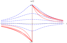

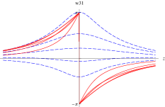
The action density also varies as function of but is periodic with a period of . At points in the middle of the intervals (108), namely at , the action density is real; otherwise it is generally complex. It is remarkable that the action itself, or the string tension, is real and does not depend on . It means that is a new string Goldstone mode, if one allows to be a function of string coordinates – in addition to the usual Goldstone modes associated with long-wave deformations of the string surface.
VI.3 Strings for higher representations,
Wilson loop in the antisymmetric rank- tensor representation is a source for functions where the numbers can lie anywhere on the circle . However, Toda equations have solutions not for all configurations of . Configurations with no classical solutions presumably give much smaller contributions to the Wilson loop at large areas than configurations that do generate solitons as they are stationary points.
The strategy for finding pinned solitons corresponding to Wilson loops in higher representations is simple: one takes the general solution (107) at certain value of and varies the phase of from to . For any there will be continuous intervals of for which the functions satisfy Toda equations (105) with a source in the r.h.s. corresponding to certain sets of numbers . For all intervals of , the pinned soliton action and hence the -string tension is given by eq. (104) and is thus degenerate in .
We did not attempt to enumerate systematically the rapidly growing variety of solitons at arbitrary
and . We find it more instructive to describe all pinned solitons of the group which is
sufficiently “rich” as it possesses non-trivial strings with and .
For the solutions have been in fact given in subsection B: six equal-length intervals of
correspond to solutions with a single source placed at
, respectively. In all cases the string tension is .
For three equal-length intervals correspond to
the double sources at ; ; ,
respectively. In all cases the string tension is .
For two equal-length intervals correspond to the triple sources at
and , respectively. In all cases the string tension is
.
As a matter of fact is a particular case of the general rank- representation of
the group. [Another example is the representation of the group,
which simultaneously is a particular case of a fundamental representation considered in
the previous subsection.] For all and there are pinned solitons generated by
sources placed at if ,
and placed at if . The string tension
is given by eq. (104) where one puts , and is degenerate in .
To summarize this section, we have shown that to find the spatial Wilson loop averaged over the ensemble of dyons, one needs to solve a chain of Toda equations with a source in the r.h.s. We have solved those equations for any and Wilson loop representation , finding pinned solitons in the transverse direction to the loop surface. The solutions generalize the famous double-layer solutions for the string in the Georgi–Glashow model by Polyakov Polyakov77 . The resulting ‘magnetic’ string tension is proportional to and coincides exactly with the ‘electric’ string tension found in Section V from the correlators of the Polyakov lines. We have observed that the Toda equations with a source allow a continuous set of solutions for the string profile, characterized by a phase , all with the same string tension. It means that in addition to the usual Goldstone modes related to deformations of the string surface, there must be an extra Goldstone mode related to the string profile. Therefore, the string theory is more complicated than given by the standard Nambu–Goto action, which may have important implications both for theory and phenomenology.
VII Summary
Generalizing previous work on the subject, we have written down the metric of the moduli space for an arbitrary number of kinds of dyons in the pure gauge theory. Assuming that it is mainly the metric and not the fluctuation determinant about dyons that defines the ensemble of interacting dyons, we have presented the grand partition function of the ensemble (where the number of particles is not fixed beforehand but found from the minimum of the free energy at given temperature) as a path integral over Abelian electric potentials and their duals , as well as over ghost fields . The resulting quantum field theory of those fields turns out to be exactly solvable owing to the cancelation between boson and ghost loops – a feature similar to that observed in supersymmetric theories. It enables one to make exact statements about the dyon ensemble: to find its free energy and correlation functions.
The free energy appears to have the minimum at the “maximal non-trivial” holonomy corresponding to the confining zero value of the average Polyakov line. Calculating the correlation functions of Polyakov lines in various -ality representations (where ) we find the asymptotic linear confining potential with the -string tension proportional to , the coefficient being calculated through the Yang–Mills scale parameter and the ’t Hooft coupling . The actual value of has to be determined self-consistently at the 2-loop level not considered here. Taking compatible with phenomenology we observe a reasonable agreement of the estimated deconfinement temperature , the string tension , the gluon condensate and the topological susceptibility with what is known from lattice simulations and phenomenology. A more robust ratio independent of and is in surprisingly good agreement with the lattice data taken at and , given the approximate nature of the model.
We have also calculated the string tension from the area law for the average of spatial Wilson loops for any and in our dyon ensemble. The spatial (‘magnetic’) string tension coincides with the ‘electric’ string tension found from Polyakov lines for all and . We find this coincidence interesting as it indicates the restoration of Lorentz symmetry at low temperatures. Since the formalism used is 3-dimensional at finite temperatures, the restoration of Lorentz symmetry at is by no means trivial.
We do not pretend we have answered all the questions and obtained a realistic confining theory as we have ignored essential ingredients of the full Yang–Mills theory, enumerated in the Introduction. Our aim was to demonstrate that the integration measure over dyons has a drastic, probably a decisive effect on the ensemble of dyons, that the ensemble can be mathematically described by an exactly solvable field theory in three dimensions, and that the resulting semiclassical vacuum built of dyons has many features expected for the confining pure Yang–Mills theory.
Acknowledgements
We thank Nikolaj Gromov and Alexei Yung for very helpful discussions. D.D. acknowledges useful discussions with Ulf Lindström, Maxim Zabzine and Konstantin Zarembo and their kind hospitality during the visit to the Theoretical Physics Department at the University of Uppsala. This work has been supported in part by the Russian Government grants RFBR-06-02-16786 and RSGSS-5788.2006.2.
References
-
(1)
E.B. Bogomolny, Yad. Fiz. 24, 861 (1976) [Sov. J.
Nucl. Phys. 24, 449 (1976)];
M.K. Prasad and C.M. Sommerfield, Phys. Rev. Lett. 35, 760 (1975). - (2) K. Lee and P. Yi, Phys. Rev. D56, 3711 (1997), ArXive: hep-th/9702107.
- (3) N.M. Davies, T.J. Hollowood, V.V. Khoze and M.P. Mattis, Nucl. Phys. B559, 123 (1999), ArXive: hep-th/9905015.
- (4) T.C. Kraan and P. van Baal, Phys. Lett. B428, 268 (1998), ArXive: hep-th/9802049; Nucl. Phys. B533, 627 (1998), ArXive: hep-th/9805168.
- (5) K. Lee and C. Lu, Phys. Rev. D58, 025011 (1998), ArXive: hep-th/9802108.
-
(6)
D. Diakonov, N. Gromov, V. Petrov and S. Slizovskiy, Phys. Rev. D70, 036003 (2004),
ArXive: hep-th/0404042;
D. Diakonov, in Continuous Advances in QCD 2004, ed. T. Ghergetta, World Scientific (2004) p. 369, ArXive: hep-ph/0407353. - (7) A. Belavin, A. Polyakov, A. Schwartz and Yu. Tyupkin, Phys. Lett. 59, 85 (1975).
- (8) B.J. Harrington and H.K. Shepard, Phys. Rev. D17, 2122 (1978); Phys. Rev. D18, 2990 (1978).
- (9) D.J. Gross, R.D. Pisarski and L.G. Yaffe, Rev. Mod. Phys. 53, 43 (1981).
-
(10)
N. Weiss, Phys. Rev. D24, 475 (1981); Phys. Rev. D25, 2667 (1982);
D. Diakonov and M. Oswald, Phys. Rev. D70, 105016 (2004), ArXive: hep-ph/0403108. - (11) D. Diakonov, Prog. Part. Nucl. Phys. 51, 173 (2003), ArXive: hep-ph/0212026.
- (12) N. Gromov and S. Slizovkiy, in preparation.
-
(13)
C. Callan, R. Dashen and D. Gross, Phys. Rev. D17, 2717 (1978);
E.M. Ilgenfritz and M. Müller-Preussker, Nucl. Phys. B184, 443 (1981);
E. Shuryak, Nucl. Phys. B203, 93 (1982);
D. Diakonov and V. Petrov, Nucl. Phys. B245, 259 (1984). -
(14)
F. Bruckmann, D. Nógrádi and P. van Baal, Nucl. Phys. B698, 233
(2004), ArXive: hep-th/0404210;
D. Nógrádi, PhD thesis, Leiden University (2005), ArXive: hep-th/0511125. - (15) M.F. Atiyah and N.J. Hitchin, Phys. Lett. A107, 21 (1985).
- (16) G.W. Gibbons and N.S. Manton, Nucl. Phys. B274, 183 (1986).
- (17) G.W. Gibbons and N.S. Manton, Phys. Lett. B356, 32 (1995).
- (18) P. Gerhold, E.M. Ilgenfritz, M. Müller-Preussker, Nucl. Phys. B760, 1 (2007); ibid. B774, 268 (2007).
- (19) K.M. Lee, E.J. Weinberg and P. Yi, Phys. Rev. D54, 1633 (1996), ArXive: hep-th/9602167; see also Ref. LeeYi .
- (20) T.C. Kraan, Commun. Math. Phys. 212, 503 (2000), ArXive: hep-th/9811179; PhD Thesis, Leiden University (2000) [available at http://www.lorentz.leidenuniv.nl/vanbaal/HOME/PUBL/kraan.ps].
-
(21)
M.F. Atiyah, V.G. Drinfeld, N.J. Hitchin and Yu.I. Manin, 65A, 185 (1978);
N.H. Christ, E.J. Weinberg and N.K. Stanton, Phys. Rev. D18, 2013 (1978);
E. Corrigan, P. Goddard and S. Templeton, Nucl. Phys. B151, 93 (1979). - (22) W. Nahm, Phys. Lett. B90 (1980) 413.
- (23) T.C. Kraan and P. van Baal, Phys. Lett. B435, 389 (1998), ArXive: hep-th/9806034.
- (24) D. Diakonov and N. Gromov, Phys. Rev. D72, 025003 (2005), ArXive: hep-th/0502132.
- (25) E. Guadagnini, Nucl. Phys. B236, 35 (1984).
- (26) D. Diakonov and V. Petrov, in: Non-perturbative approaches to Quantum Chromodynamics, Proc. int. workshop at ECT*, Trento, 1995, ed. D. Diakonov, Gatchina (1995) p. 36, ArXive: hep-th/9606104.
-
(27)
G. ’t Hooft, Phys. Rev. D14, 3432 (1976); Erratum: ibid. D18, 2199
(1978);
C. Bernard, Phys. Rev. D19, 3013 (1979). - (28) G.W. Gibbons and C.N. Pope, Commun. Math. Phys. 66, 267 (1979).
- (29) M.F. Atiyah and N.J. Hitchin, The Geometry and Dynamics of Magnetic Monopoles, Princeton University Press (1988).
- (30) The definition of the metric tensor is the matrix composed of zero modes’ overlaps. At large separations between dyons, the four approximately zero modes per dyon are where is the field strength of the dyon whose scale parameter has to be adjusted by the Coulomb field of other dyons. This is why the first correction to the metric is always Coulomb-like. It is remarkable that for different-kind dyons there are no further corrections.
- (31) N. Gromov, ArXive: hep-th/0701192.
- (32) D. Diakonov and V. Petrov, Ref. ILM .
- (33) F.A. Berezin, Second Quantization Method, Nauka, Moscow (1965) (in Russian).
- (34) A. Polyakov, Nucl. Phys. B120, 429 (1977).
- (35) In principle, one can think of a quantum anomaly leading to an uncomplete cancellation of boson and ghost determinants, as it happens in some supersymmetric examples Shifman-Yung . We do not see a reason for the anomaly in our case, however. Therefore, unless proven otherwise, we shall assume that the cancellation is exact.
- (36) M. Shifman and A. Yung, ArXive: hep-th/0703267.
- (37) S. Jaimungal and A.R. Zhitnitsky, ArXive: hep-ph/9905540; A.R. Zhitnitsky, ArXive: hep-ph/0601057.
- (38) M. Toda, Phys. Rep. 18C, 1 (1975). It should be noticed, however, that the classic Toda lattice is of the “hyperbolic” type, i.e. the sign in the definition of (49) is opposite. Here the Toda lattice is of the “elliptic” type.
- (39) Temperature dependence of the string tension appears when one adds e.g. the perturbative potential energy into consideration. Since its relative contribution is one expects that it modifies seriously eq. (88) only close to the phase transition temperature where the electric string tension vanishes.
-
(40)
B. Lucini, M. Teper and U. Wenger, JHEP 0401, 061 (2003), ArXive: hep-lat/0307017;
B. Lucini, M. Teper and U. Wenger, ArXive: hep-lat/0502003. - (41) B. Lucini and M. Teper, ArXive: hep-lat/0103027.
- (42) D. Diakonov and V. Petrov, Phys. Rev. D67, 105007 (2003), ArXive: hep-th/0212018.
- (43) M. Shifman, Acta Phys. Polon. B6, 3805 (2005), ArXive: hep-th/0510098.
-
(44)
M.R. Douglas and S.H. Shenker, Nucl. Phys. B447, 271 (1995);
A. Hanany, M. Strassler and A. Zaffaroni, Nucl. Phys. B513, 87 (1998), ArXive: hep-th/9707244. - (45) In our linearized approach, there are combinatorial contributions to the correlator, stemming from expanding the exponent in eq. (83) and its analogs for arbitrary in higher powers of . Starting from there is a danger that a combination of lower eigenvalues may give a larger contribution to the correlator than a single contribution of , for example, . For this particular case we have proved that the square of the contribution decouples from the correlator for all . However, we have not proved it for all and all possible combinations of eigenvalues whose sum is less than : probably certain generalizations of the orthogonality relations (96) are responsible for it. A more appropriate approach would be to solve the full non-linear equations. We note that combinatorial contributions leading to larger string tensions are generally present and can be considered as string excitations.
- (46) L. Del Debbio, H. Panagopoulos, P. Rossi and E. Vicari, JHEP 0201, 009 (2002), ArXive: hep-th/0111090.
- (47) B. Lucini, M. Teper and U. Wenger, JHEP 0406, 012 (2004), ArXive: hep-lat/0404008.
- (48) T.J. Hollowood, ArXive: hep-th/9110010.