The causal boundary of product spacetimes

Abstract.

The new formulation of the causal completion of spacetimes suggested in [1], and modified later in [2], is tested by computing the causal boundary for product spacetimes of a Lorentz interval and a Riemannian manifold. This is particularized for two important families of spacetimes, conformal to the previous ones: (standard) static spacetimes and Generalized Robertson-Walker spacetimes. As consequence, it is shown that this new approach essentially reproduces the structure of the conformal boundary for multiple classical spacetimes: Reissner-Nordstrom (including Schwarzschild), Anti-de Sitter, Taub and standard cosmological models as de Sitter and Einstein Universe.

Keywords: boundary on spacetime, causal boundary, Busemann function, (standard) static spacetimes, Generalized Robertson-Walker spacetimes.
2000 MSC: 53C50, 83C75

1 Introduction

In the last decades, relativists have shown great interest in certain remarkable properties related to the asymptotic behavior of spacetimes, as singularities. In order to get a better understanding of these phenomenons, sometimes it is very useful to attach a sort of ideal boundary to the spacetime. However, the construction of the ‘optimal’ boundary has shown to be a very elusive problem up to date.

A well-known boundary in Relativity is the conformal boundary [3], which consists of conformally embedding the original spacetime into a larger one, and then, taking the boundary of the image. However, this method is neither systematic nor intrinsic, and sometimes it results very restrictive. In order to overcome these handicaps, Geroch, Kronheimer and Penrose introduced a new construction called causal boundary [4]. In this new approach they attach a future (past) ideal point for every inextensible, physically admissible future (past) trajectory, in such a way that the ideal point only depends on the past (future) of the trajectory. In fact, this method is systematic, intrinsic and very general. However, it suffers from an important technical difficulty: in general, some future and past ideal points must be identified in order to avoid pathologies derived from having ‘too big’ boundaries.

Many authors have tried different methods to establish these identifications [4, 5, 6, 7]; indeed, this question is related to the introduction of a satisfactory topology for the completion. However, they have not obtained totally satisfactory results up to date (see [8, 9, 10, 1]). See also [11], [12] for interesting reviews on the subject.

Based on a new formulation by Marolf and Ross [1], which replace the identifications by pairs representing the ideal points, recently the second author has developed a new approach to the causal boundary with promising results [2]. This approach lies on a ‘minimality principle’ which allows to establish the desired pairs, in addition to a reasonable topology for the completion. As consequence, it is obtained a construction with many satisfactory mathematical properties. However, this construction has not been checked in many spacetimes of physical interest.

In this paper we are going to test this new formulation by computing the causal boundary for some physically relevant spacetimes. After a preliminary section devoted to recall some basic notions on causal structure and causal completions, in Section 3 we construct the causal boundary for product spacetimes of a Lorentz interval and a Riemannian manifold. In Section 4 we use the conformal invariance of the causal boundary to directly deduce the boundary for two important families in the conformal class: (standard) static spacetimes and Generalized Robertson-Walker spacetimes. As consequence, we describe the boundary for multiple classical spacetimes in these families: Reissner-Nordstrom (including Schwarzschild), Anti-de Sitter, Taub and standard cosmological models as de Sitter and Einstein Universe. Finally, in Section 5 we summarize the main conclusions, putting special emphasis in the fact that this approach essentially reproduces the structure of the conformal boundary for these examples.

2 Preliminaries

Let $(V,g)$ be a spacetime, i.e. a connected smooth manifold $V$ endowed with metric tensor $g$ of index $1$. A tangent vector $v\in T_{p}V$, $p\in V$ is named timelike (resp. lightlike; spacelike; causal) if $g(v,v)<0$ (resp. $g(v,v)=0$ and $v\neq 0$; $g(v,v)>0$ or $v=0$; $v$ is either timelike or lightlike). Accordingly, a smooth curve $\gamma:I\rightarrow V$ ($I$ real interval) is called timelike (resp. lightlike; spacelike; causal) if $\gamma^{\prime}(s)$ is timelike (resp. lightlike; spacelike; causal) for all $s$. Spacetimes are assumed to be time-orientable, i.e. they must admit a time-orientation, which is a continuous, globally defined, timelike vector field $X$. Fixed a time-orientation $X$, a causal curve $\gamma(s)$ is said future-directed (resp. past-directed) if $g(\gamma^{\prime}(s),X(\gamma(s)))<0$ (resp. $g(\gamma^{\prime}(s),X(\gamma(s)))>0$) for all $s$. Future-directed causal curves represent all the physically admissible trajectories for material particles and light rays in the universe.

Two events $p,q\in V$ are chronologically related $p\ll q$ (resp. causally related $p\prec q$) if there exists some future-directed timelike (resp. causal) curve from $p$ to $q$. If $p\prec q$ but $p\not\ll q$, they are said horismotically related $p\rightarrow q$. The chronological past of $p$, $I^{-}(p)$, (resp. causal past of $p$, $J^{-}(p)$) is defined as:

$$I^{-}(p)=\{q\in V:q\ll p\}\qquad(\hbox{resp.}\;\;J^{-}(p)=\{q\in V:q\prec p\}).$$

Of course, the chronological future of $p$, $I^{+}(p)$ (resp. causal future of $p$, $J^{+}(p)$) is defined by replacing $q\ll p$ (resp. $q\prec p$) by $p\ll q$ (resp. $p\prec q$) in previous definition.

The main purpose of the causal completion of spacetimes is to avoid the existence of inextensible timelike curves. This is overcome by adding ideal points to the spacetime in such a way that any timelike curve presents some endpoint in the new space. In order to rigorously describe this completion, applicable to strongly causal spacetimes (i.e. spacetimes without closed or ‘nearly closed’ timelike curves), previously we need to introduce some terminology:

A subset $P\subset V$ is called past set if it coincides with its past, which is always open; i.e. $P=I^{-}[P]:=\{p\in V:p\ll q\;\hbox{for some}\;q\in P\}$. Given a subset $S\subset V$, the common past of $S$ is defined by $\downarrow S:=I^{-}[\{p\in V:\;\;p\ll q\;\;\forall q\in S\}]$. A past set that cannot be written as the union of two proper subsets, both of which are also past sets, is called indecomposable past set, IP. An IP which does not coincide with the past of any point in $V$ is called terminal indecomposable past set, TIP. Otherwise, it is called proper indecomposable past set, PIP. By interchanging the roles of past and future, we obtain the corresponding notions for future set, common future, IF, TIF and PIF.

In order to construct the future causal completion, first identify every event $p\in V$ with its PIP, $I^{-}(p)$. Then, the future causal boundary $\hat{\partial}(V)$ of $V$ is defined as the set of all TIPs in $V$. Therefore, the future causal completion $\hat{V}$ becomes the set of all IPs:

$$V\equiv\hbox{PIPs},\qquad\hat{\partial}(V)\equiv\hbox{TIPs},\qquad\hat{V}\equiv\hbox{IPs}.$$

Analogously, every event $p\in V$ can be identified with its PIF, $I^{+}(p)$. Then, the past causal boundary $\check{\partial}(V)$ of $V$ is defined as the set of all TIFs in $V$, and thus, the past causal completion $\check{V}$ is the set of all IFs:

$$V\equiv\hbox{PIFs},\qquad\check{\partial}(V)\equiv\hbox{TIFs},\qquad\check{V}\equiv\hbox{IFs}.$$

For the (total) causal completion, one immediately thinks of the space $\hat{V}\cup\check{V}$. However, it becomes evident that by only imposing the obvious identifications $I^{-}(p)\sim I^{+}(p)$ on $\hat{V}\cup\check{V}$ for all $p\in V$, the resulting space $V^{\natural}$ does not provide a satisfactory description for the boundary of $V$: in fact, this procedure often attaches two ideal points where we would expect only one.

The first attempt to establish identifications in $\hat{\partial}(V)\cup\check{\partial}(V)$ was proposed in [4]. The authors introduced a generalized Alexandrov topology on $V^{\natural}$: the topology generated by the sub-basis

$$\begin{array}[]{l}A^{int}=\{P\in\hat{V}:P\cap A\neq\emptyset\}\\ A^{ext}=\{P\in\hat{V}:P=I^{-}[W]\;\;\hbox{implies}\;\;I^{+}[W]\nsubseteq A\}\end{array}\qquad\hbox{for all}\;\;A\in\check{V},$$

$$\begin{array}[]{l}B^{int}=\{F\in\check{V}:F\cap B\neq\emptyset\}\\ B^{ext}=\{F\in\check{V}:F=I^{+}[W]\;\;\hbox{implies}\;\;I^{-}[W]\nsubseteq B\}\end{array}\qquad\hbox{for all}\;\;B\in\hat{V}.$$

Then, they suggested the minimum set of identifications necessary to obtain a Hausdorff space. However, this method fails to produce the ‘expected’ structure and topology for the completion in some examples [8], [9], [13], [1, Sect. 5]. As commented before, other more accurate attempts have been suggested since then, but without totally satisfactory results.

An alternative procedure to making identifications consists of forming pairs composed by past and future indecomposable sets of $V$. This approach, firstly introduced in [1] and developed later in [2], has exhibited satisfactory results for those spacetimes analyzed up to date (see [1, 2, 14]). In this paper we are going to test this approach for product spacetimes.

Even if the criteria proposed in [1] and [2] for pairing terminal sets are different in general, they coincide in many cases. In particular, they coincide for those spacetimes such that every terminal set is not S-related (Szabados related) with more than one terminal set: we say that $P,F$ are S-related, $P\sim_{S}F$, if $P$ is maximal IP into $\downarrow F$ and $F$ is maximal IF into $\uparrow P$. For these spacetimes, the construction in [2, Th. 7.4] reduces to the following definition coming from [1, Def. 4]:

Definition 2.1

The (total) causal boundary $\overline{V}$ is formed by all the pairs $(P,F)$ formed by a TIP $P$ and a TIF $F$ such that: either $P\sim_{S}F$; or $P=\emptyset$ and there is no $P^{\prime}\neq\emptyset$ such that $P^{\prime}\sim_{S}F$; or $F=\emptyset$ and there is no $F^{\prime}\neq\emptyset$ such that $P\sim_{S}F^{\prime}$.

This will be the definition adopted in this paper, since product spacetimes always satisfy the property above (Remark 3.5).

With this definition, the causal structure of the spacetime can be easily extended to the completion. Concretely, we say that $(P,F),(P^{\prime},F^{\prime})\in\overline{V}$ are chronologically related, $(P,F)\ll(P^{\prime},F^{\prime})$, if $F\cap P^{\prime}\neq\emptyset$. Here, $(P,F)$, $(P^{\prime},F^{\prime})$ will be said causally related, $(P,F)\prec(P^{\prime},F^{\prime})$, if $F^{\prime}\subset F$ and $P\subset P^{\prime}$. Finally, $(P,F)$, $(P^{\prime},F^{\prime})$ are horismotically related, $(P,F)\rightarrow(P^{\prime},F^{\prime})$, if they are causally, but not chronologically, related.

The topology of the spacetime can be also extended to the completion. Here we adopt the so called chronological topology, firstly introduced in [2]. This topology is defined in terms of the following limit operator $L$: given a sequence $\sigma=\{(P_{n},F_{n})\}\subset\overline{V}$, we say that $(P,F)\in L(\sigma)$ if

$$\begin{array}[]{c}P\in\hat{L}(P_{n}):=\{P^{\prime}\in\hat{V}:P^{\prime}\subset{\rm LI}(P_{n})\;\;\hbox{and}\;\;P^{\prime}\;\;\hbox{is maximal IP into}\;\;{\rm LS}(P_{n})\}\\ F\in\check{L}(F_{n}):=\{F^{\prime}\in\check{V}:F^{\prime}\subset{\rm LI}(F_{n})\;\;\hbox{and}\;\;F^{\prime}\;\;\hbox{is maximal IF into}\;\;{\rm LS}(F_{n})\}.\end{array}$$ (2.1)

Then, the closed sets for the chronological topology are those subsets $C\subset\overline{V}$ such that $L(\sigma)\subset C$ for any sequence $\sigma\subset C$.

Finally, we remark that the causal boundary is conformally invariant, i.e. it remains unaltered under conformal transformations of the spacetime.

3 Causal boundary for product spacetimes

We consider product spacetimes $(V,g)$ of a Lorentz interval $(I,-dt^{2})$, $I=(a,b)\subseteq{\mathbb{R}}$ and a Riemannian manifold $(M,h)$:

$$V=I\times M,\qquad g=-dt^{2}+h.$$ (3.1)

Here, the time orientation is determined by $\partial_{t}$. Of course, these spacetimes are always strongly causal, and thus, the causal completion applies. In order to construct the causal boundary of these spacetimes, we have followed several steps. By completeness, we have included here some arguments and results coming from [15].

$\S$1. Computation of PIPs and PIFs:

We begin by computing the PIPs and PIFs. If $(t_{0},x_{0})\ll(t_{1},x_{1})$ then there exists a timelike curve $\gamma(s)=(t(s),c(s))$ such that $\gamma(0)=(t_{0},x_{0})$, $\gamma(1)=(t_{1},x_{1})$. Since $\gamma$ is timelike, necessarily $\dot{t}(s)>\sqrt{h(\dot{c}(s),\dot{c}(s))}$ for all $s$. In particular,

$$t_{1}-t_{0}=\int_{0}^{1}\dot{t}(s)ds>\int_{0}^{1}\sqrt{h(\dot{c}(s),\dot{c}(s))}=\hbox{long}(c)\geq d(x_{0},x_{1}),$$

being $d$ the distance in $M$ associated to $h$. Reciprocally, if $t_{1}-t_{0}>d(x_{0},x_{1})$ then there exists a curve $c(s)$ in $M$ with $c(0)=x_{0}$, $c(1)=x_{1}$ such that $|\dot{c}(s)|<t_{1}-t_{0}$ for all $s$. Therefore, the curve $\gamma(s)=(t(s),c(s))$, with $t(s)=(t_{1}-t_{0})s+t_{0}$, is timelike and satisfies $\gamma(0)=(t_{0},x_{0})$, $\gamma(1)=(t_{1},x_{1})$, proving that $(t_{0},x_{0})\ll(t_{1},x_{1})$. Summarizing:

$$(t_{0},x_{0})\ll(t_{1},x_{1})\Longleftrightarrow t_{0}<t_{1}-d(x_{0},x_{1}).$$ (3.2)

This property directly provides the following result:

Proposition 3.1

The PIPs and PIFs of product spacetime (3.1) are:

$$\begin{array}[]{c}I^{-}(p)=\{(t^{\prime},x^{\prime})\in I\times M:t^{\prime}<d^{t}_{x}(x^{\prime})\}\\ I^{+}(p)=\{(t^{\prime},x^{\prime})\in I\times M:t^{\prime}>-d^{-t}_{x}(x^{\prime})\}\end{array}\quad\hbox{for all}\;\;p=(t,x)\in I\times M,$$ (3.3)

being $d^{t}_{x}(\cdot):=t-d(\cdot,x)$.

$\S$2. Computation of TIPs and TIFs:

To this aim, we only need to compute the past and future of inextensible timelike curves (see, for example, [16, Prop. 6.14]). So, let $\gamma(s)=(t(s),c(s))$ be an inextensible future-directed timelike curve. In particular, $\dot{t}(s)>0$ for all $s$, and thus, we can reparametrize $\gamma$ by $t$ in order to obtain $\gamma(t)=(t,c(t))$, where now the spatial projection $c$ is a curve with domain some interval $[w,\Omega)$, $\Omega\leq b$ and velocity $|\dot{c}|<1$. The following definition will be useful:

Definition 3.2

We define the Busemann function of such a curve $c$ as the function:

$$b_{c}:M\rightarrow{\mathbb{R}}^{*}\equiv{\mathbb{R}}\cup\{\infty\},\quad b_{c}(\cdot):=\lim_{t\rightarrow\Omega}d^{t}_{c(t)}(\cdot)=\lim_{t\rightarrow\Omega}(t-d(\cdot,c(t))).$$

Recall that the past of $\gamma$ coincides with the union of the pasts $I^{-}(\gamma(t))$ $\,\forall t\in[w,\Omega)$. Therefore, $(t^{\prime},x^{\prime})\in I^{-}[\gamma]$ if and only if $(t^{\prime},x^{\prime})\in I^{-}(\gamma(t))$ for some $t$ close enough to $\Omega$ (observe that $I^{-}(\gamma(t_{1}))\subset I^{-}(\gamma(t_{2}))$ if $t_{1}<t_{2}$). Taking into account (3.3), this condition translates into the following inequality:

$$t^{\prime}<\lim_{t\rightarrow\Omega}d^{t}_{c(t)}(x^{\prime})=b_{c}(x^{\prime}).$$

If $\gamma(t)=(-t,c(t))$ is an inextensible past-directed timelike curve, analogous arguments can be applied (just interchange the roles of future and past) in order to obtain: $(t^{\prime},x^{\prime})\in I^{+}[\gamma]$ if and only if

$$t^{\prime}>\lim_{t\rightarrow\Omega}(-d^{t}_{c(t)}(x^{\prime}))=-b_{c}(x^{\prime}).$$

Summarizing, we can establish the following result:

Proposition 3.3

The TIPs (TIFs) of product spacetime (3.1) are:

$$\begin{array}[]{c}I^{-}[\gamma]=\{(t^{\prime},x^{\prime})\in I\times M:t^{\prime}<b_{c}(x^{\prime})\}\\ (I^{+}[\gamma]=\{(t^{\prime},x^{\prime})\in I\times M:t^{\prime}>-b_{c}(x^{\prime})\})\end{array}$$

for any inextensible future (past) timelike curve $\gamma$.

$\S$3. Partial boundaries:

The structure of the partial boundaries can be analyzed in terms of the extremes of the interval:

Case $b=\infty$. Any inextensible curve $\gamma$ with component $c$ approaching to some $x_{0}\in M$ satisfy $\Omega=\infty$. Moreover, in this case $b_{c}\equiv\infty$. Therefore, from Proposition 3.3 these curves satisfy

$$I^{-}[\gamma]=V.$$

This TIP corresponds to the future timelike infinity, and is labeled by $i^{+}$. The rest of TIPs are univocally determined by all the finite Busemann functions $b_{c}<\infty$ in $(M,h)$ associated to inextensible components $c$ of curves $\gamma$. Therefore, if ${\cal B}(M)$ denotes the set of all these finite Busemann functions, then we have:

$$\hat{\partial}(V)={\cal B}(M)\cup\{\infty\}.$$

The set ${\cal B}(M)$ is invariant under the additive action: if $b_{c}\in{\cal B}(M)$ then $b_{c}+k\in{\cal B}(M)$ for all $k\in(a-\Omega,\infty)$ (in fact, $b_{c^{\prime}}=b_{c}+k$ if $c^{\prime}(t):=c(t-k)$). Therefore, if we define the Busemann boundary as the quotient

$$\partial_{B}(M):={\cal B}(M)/(a,\infty),$$

then it is

$$\hat{\partial}(V)={\cal B}(M)\cup\{\infty\}\equiv(\partial_{B}(M)\times(a,\infty))\cup\{i^{+}\}.$$

It should be remarked that $\partial_{B}(M)$ includes two types of elements. Those points associated to inextensible curves $c$ with $\Omega=\infty$, which can be interpreted as ‘infinity directions’ of the manifold $(M,h)$; and those points associated to inextensible curves $c$ with $\Omega<\infty$, which define points of the Cauchy boundary $\partial_{C}(M)$ of the manifold. In this last case we have $b_{c}=d_{x_{0}}^{\Omega}$, $x_{0}\in\partial_{C}(M)$.

Case $b<\infty$. Now $\Omega<\infty$, and thus, $b_{c}<\infty$ for any $c$. In particular, $i^{+}$ does not belong to the future boundary of the spacetime. Indeed, every inextensible curve $\gamma$ with $c$ approaching to some $x_{0}\in M$, and thus, $\Omega=b$, has Busemann function $b_{c}=d^{b}_{x_{0}}<\infty$. As consequence, the future boundary contains a copy of $M$. The rest of TIPs are univocally determined by all the finite Busemann functions $b_{c}<\infty$ associated to inextensible components $c$ of curves $\gamma$. We denoted this set by ${\cal B}(M)$. Arguing as before, ${\cal B}(M)$ is invariant by the additive action: if $b_{c}\in{\cal B}(M)$ then $b_{c}+k\in{\cal B}(M)$ for all $k\in(a-\Omega,b-\Omega]$. Therefore:

$$\hat{\partial}(V)={\cal B}(M)\cup M\equiv(\partial_{B}(M)\times(a,b])\cup M\equiv(\partial_{C}(M)\times(a,b])\cup M.$$

If we repeat the arguments above, but now interchanging the roles of future and past, we obtain the corresponding results for the past boundaries in terms of the extreme $a$. That is:

Case $a=-\infty$. Now $\check{\partial}(V)={\cal B}(M)\cup\{-\infty\}\equiv(\partial_{B}(M)\times(-\infty,b))\cup\{i^{-}\}$, where $i^{-}$ labels the TIF $V$ corresponding to the past timelike infinity.

Case $a>-\infty$. Now $\check{\partial}(V)={\cal B}(M)\cup M\equiv(\partial_{C}(M)\times[a,b))\cup M$.

$\S$4. The (total) causal boundary:

In order to construct the (total) causal boundary from the partial boundaries, we need to know which TIPs $P$ and TIFs $F$ are S-related. The following lemma solves this question:

Lemma 3.4

Two terminal sets $P,F\neq\emptyset$ of $V$ satisfy $P\sim_{S}F$ iff for some $x_{0}\in\partial_{C}(M)$

$$P=\{(t^{\prime},x^{\prime}):t^{\prime}<d^{\Omega}_{x_{0}}(x^{\prime})\},\quad F=\{(t^{\prime},x^{\prime}):t^{\prime}>-d^{-\Omega}_{x_{0}}(x^{\prime})\},\quad a<\Omega<b.$$ (3.4)

Proof. Suppose that $P\sim_{S}F$, with $P,F\neq\emptyset$. Let $\gamma_{+}:[w,\Omega)\rightarrow V$, $\gamma_{+}(t)=(t,c_{+}(t))$ be an inextensible future-directed timelike curve such that $P=I^{-}[\gamma_{+}]$. Since $\uparrow P\supset F\neq\emptyset$ and coordinate $t$ strictly increases along future-directed timelike curves, necessarily $\Omega<b$. Moreover, since $\gamma_{+}$ is inextensible, necessarily $c_{+}(t)\rightarrow x_{0}\in\partial_{C}(M)$. Analogously, $F=I^{+}[\gamma_{-}]$, where $\gamma_{-}:[w^{\prime},\Omega^{\prime})\rightarrow V$, $\gamma_{-}(t)=(-t+2\Omega^{\prime},c_{-}(t))$, is an inextensible past-directed timelike curve such that $c_{-}(t)\rightarrow x^{\prime}_{0}\in\partial_{C}(M)$ and $\Omega^{\prime}>a$. Summarizing:

$$P=\{(t^{\prime},x^{\prime}):t^{\prime}<d^{\Omega}_{x_{0}}(x^{\prime})\},\quad F=\{(t^{\prime},x^{\prime}):t^{\prime}>-d^{-\Omega^{\prime}}_{x^{\prime}_{0}}(x^{\prime})\},$$

being $a<\Omega,\Omega^{\prime}<b$ and $x_{0},x^{\prime}_{0}\in\partial_{C}(M)$. Moreover, it is $d(x_{0},x^{\prime}_{0})\leq\Omega^{\prime}-\Omega$, since, otherwise, we can take $\overline{\Omega}^{\prime}>\Omega^{\prime}$ and $\overline{\Omega}<\Omega$ such that $d(x_{0},x^{\prime}_{0})>\overline{\Omega}^{\prime}-\overline{\Omega}$, which implies $(\overline{\Omega},x_{0})\in P$, $(\overline{\Omega}^{\prime},x^{\prime}_{0})\in F$ but $(\overline{\Omega},x_{0})\not\ll(\overline{\Omega}^{\prime},x^{\prime}_{0})$, in contradiction with $F\subset\uparrow P$. Finally, notice also that $\Omega=\Omega^{\prime}$, and thus, $x_{0}=x^{\prime}_{0}$. In fact, take any $x_{0}\in\overline{M}_{C}$ and $\Omega<\overline{\Omega}<\Omega^{\prime}$ such that $d(x_{0},\overline{x}_{0})=\overline{\Omega}-\Omega$ and $d(x^{\prime}_{0},\overline{x}_{0})=\Omega^{\prime}-\overline{\Omega}$. Then, $\overline{F}:=\{(t^{\prime},x^{\prime}):t^{\prime}>-d_{\overline{x}_{0}}^{-\overline{\Omega}}(x^{\prime})\}$ satisfies $F\varsubsetneq\overline{F}\subseteq\uparrow P$, which contradicts the maximality of $F$ into $\uparrow P$.

Assume now that (3.4) holds for some $x_{0}\in\partial_{C}(M)$. If $(t,x)\in F$ then $t-\Omega>d(x,x_{0})$, which implies $(t,x)\in\uparrow P$. Therefore, $F\subset\uparrow P$. Moreover, $F$ is maximal into $\uparrow P$, since, otherwise, there would exist $(t,x)\neq(\Omega,x_{0})$ satisfying $t-\Omega\geq d(x,x_{0})$ and $\Omega-t\geq d(x,x_{0})$, a contradiction. Analogously, we can prove that $P$ is maximal into $\downarrow F$. Whence, $P\sim_{S}F$. $\Box$

Remark 3.5

In particular, this shows that every terminal set is not S-related with more than one terminal set.

From Definition 2.1, Lemma 3.4 and Remark 3.5, we deduce the following result:

Proposition 3.6

The causal boundary $\partial(V)$ of $V$ can be written as the union of the corresponding partial boundaries $\hat{\partial}(V)$, $\check{\partial}(V)$, with each pair of lines in $\hat{\partial}(V)$, $\check{\partial}(V)$ based on the same point of $\partial_{C}(M)$ identified.

$\S$5. Causal structure and topology for the boundary:

The causal relations between ideal points are given by this proposition:

Proposition 3.7

Let $V=(a,b)\times M$, $g=-dt^{2}+h$ be a product spacetime. Then:

• The lines of the boundary based on points in $\partial_{B}(M)\setminus\partial_{C}(M)$ are null (i.e. any two points on the line are horismotically related).

• The lines of the boundary based on points in $\partial_{C}(M)$ are timelike (i.e. any two points on the line are chronologically related).

• The copies of $M$ in the boundary are spacelike (i.e. any two points on the copy are not causally related).

Proof. (i) Let $(P,\emptyset)$, $(P^{\prime},\emptyset)$ be two elements of the boundary lying on some line based on some point in $\partial_{B}(M)\setminus\partial_{C}(M)$. Then, it is not a restriction to assume

$$P=\{(t^{\prime},x^{\prime}):t^{\prime}<b_{c}(x^{\prime})\},\quad P^{\prime}=\{(t^{\prime},x^{\prime}):t^{\prime}<b_{c^{\prime}}(x^{\prime})\},\quad\hbox{being}\;b_{c^{\prime}}=b_{c}+k,\;k>0.$$

Therefore, $P\varsubsetneq P^{\prime}$, which proves that $(P,\emptyset)$ and $(P^{\prime},\emptyset)$ are causally related. On the other hand, the equality $\emptyset\cap P^{\prime}=\emptyset$ implies that they are not chronologically related. Whence $(P,\emptyset)$ and $(P^{\prime},\emptyset)$ are horismotically related.

(ii) Let $(P,F)$, $(P^{\prime},F^{\prime})$ be two elements of the boundary lying on some line based on some point $x_{0}\in\partial_{C}(M)$. We can assume that

$$F=\{(t^{\prime},x^{\prime}):t^{\prime}>-d^{-\Omega}_{x_{0}}(x^{\prime})\},\;\;P^{\prime}=\{(t^{\prime},x^{\prime}):t^{\prime}<d^{\Omega^{\prime}}_{x_{0}}(x^{\prime})\},\;\;\hbox{being}\;\,a\leq\Omega<\Omega^{\prime}\leq b.$$

As consequence, if $\overline{\Omega}=\Omega+(\Omega^{\prime}-\Omega)/2$ and $x\in M$ is such that $d(x,x_{0})<(\Omega^{\prime}-\Omega)/2$, then $\overline{\Omega}>-d_{x_{0}}^{-\Omega}(x)$, $\overline{\Omega}<d_{x_{0}}^{\Omega^{\prime}}(x)$, and thus, $(\overline{\Omega},x)\in P^{\prime}\cap F\neq\emptyset$. Whence, $(P,F)$ and $(P^{\prime},F^{\prime})$ are chronologically related.

(iii) For example, let $(P,\emptyset)\neq(P^{\prime},\emptyset)$ be two elements of some copy of $M$ in the boundary. Then $P=I^{-}[\gamma_{+}]$ for some inextensible timelike curve $\gamma_{+}:[w,b)\rightarrow V$, $\gamma_{+}(t)=(t,c_{+}(t))$, $c_{+}(t)\rightarrow x_{0}\in M$, and $P^{\prime}=I^{-}[\gamma^{\prime}_{+}]$ for some inextensible timelike curve $\gamma^{\prime}_{+}:[w,b)\rightarrow V$, $\gamma^{\prime}_{+}(t)=(t,c^{\prime}_{+}(t))$, $c^{\prime}_{+}(t)\rightarrow x^{\prime}_{0}\in M$, $x_{0}\neq x^{\prime}_{0}$. In particular, $t>d_{x_{0}}^{b}(c^{\prime}_{+}(t))$, $t>d^{b}_{x^{\prime}_{0}}(c_{+}(t))$ for all $t$ close enough to $b<\infty$. Whence, $P\nsubseteq P^{\prime}$, $P^{\prime}\nsubseteq P$, which implies that $(P,\emptyset)$, $(P^{\prime},\emptyset)$ are not causally related. $\Box$

Finally, the topology for the causal completion is directly deduced from the definition of limit operator $L$ in terms of $\hat{L}$ and $\check{L}$ (formulae (2.1)):

Proposition 3.8

The chronological topology on $\overline{V}$ coincides with the quotient topology under $\sim_{S}$ of the topology generated by the limit operators $\hat{L}$ and $\check{L}$ on $\hat{V}\cup\check{V}$.

$\S$6. Main result:

All these propositions, joined to the following result from [17, Prop. 6.7, Sect. 6.1.3], yield our main statement, Theorem 3.10.

Proposition 3.9

Let $M=(\alpha,\omega)\times_{a}K$ be a Riemannian manifold with $(\alpha,\omega)\subseteq{\mathbb{R}}$, $a:(\alpha,\omega)\rightarrow{\mathbb{R}}$ a positive function, $K$ a compact manifold, and metric given by $h=d\rho^{2}+a(\rho)^{2}j_{K}$ (being $j_{k}$ the metric on $K$). For some $\rho_{-}<\rho_{+}$ in $(\alpha,\omega)$, assume that $a(\rho)$ is decreasing in $\rho\in(\alpha,\rho_{-}]$ and increasing in $\rho\in[\rho_{+},\omega)$, or increasing in the whole $(\alpha,\omega)$ with $a(\alpha)=0$, $\alpha=0$. Then $\partial_{B}(M)$ is formed by two spaces $B_{\alpha}$ and $B_{\omega}$, attached at $\{\alpha\}\times K$ and $\{\omega\}\times K$, resp., with each $B_{\imath}$ ($\imath=\alpha,\omega$) being $K$ or an unique point $\ast$: concretely, $B_{\imath}\cong K$ if $|\int_{\rho_{0}}^{\imath}1/a(\rho)^{2}d\rho|<\infty$, and $B_{\imath}=\ast$ if $|\int_{\rho_{0}}^{\imath}1/a(\rho)^{2}d\rho|=\infty$. Moreover, $B_{\imath}$ belongs to $\partial_{C}(M)$ if and only if the extreme $\imath$ is finite.

Theorem 3.10

Let $V=(a,b)\times M$, $g=-dt^{2}+h$ be a product spacetime whose spatial part $(M,h)$ falls under the hypotheses of Proposition 3.9. Then, the causal boundary of $(V,g)$ admits the following structure (with the chronological topology):

• If $-\infty=a<b=\infty$ then it is formed by two infinity null cones, one for the future and another for the past, with base $\partial_{B}(M)\setminus\partial_{C}(M)$ and apexes $i^{+}$ and $i^{-}$, resp., and timelike lines of future and past extremes $i^{+}$ and $i^{-}$, resp., on each point of $\partial_{C}(M)$ (Figure 1).

• If $-\infty<a<b<\infty$ then it is formed by two copies, one for the future and another for the past, of the Cauchy completion $\overline{M}_{C}$ of $(M,h)$, and timelike lines based on each point of $\partial_{C}(M)$ which connect both copies (Figure 2).

• If $-\infty<a<b=\infty$ then it is formed by an infinity null cone for the future with base $\partial_{B}(M)\setminus\partial_{C}(M)$ and apex $i^{+}$, a copy of $\overline{M}_{C}$ for the past, and timelike lines based on each point of $\partial_{C}(M)$ which connect $\overline{M}_{C}$ with $i^{+}$ (Figure 3).

• If $-\infty=a<b<\infty$ then it is formed by an infinity null cone for the past with base $\partial_{B}(M)\setminus\partial_{C}(M)$ and apex $i^{-}$, a copy of $\overline{M}_{C}$ for the future, and timelike lines based on each point of $\partial_{C}(M)$ which connect $i^{-}$ with $\overline{M}_{C}$ (Figure 4).

Moreover, $\partial_{B}(M)$ is formed by two spaces $B_{\alpha}$ and $B_{\omega}$, attached at $\{\alpha\}\times K$ and $\{\omega\}\times K$, resp., with each $B_{\imath}$ ($\imath=\alpha,\omega$) being $K$ or an unique point $\ast$: concretely, $B_{\imath}\cong K$ if $|\int_{\rho_{0}}^{\imath}1/a(\rho)^{2}d\rho|<\infty$, and $B_{\imath}=\ast$ if $|\int_{\rho_{0}}^{\imath}1/a(\rho)^{2}d\rho|=\infty$. Finally, $B_{\imath}$ belongs to the Cauchy boundary $\partial_{C}(M)$ if and only if the extreme $\imath$ is finite.

In particular, Theorem 3.10 shows that the causal boundary of a product spacetime is exclusively determined by the Busemann boundary $\partial_{B}(M)$ (and the Cauchy boundary $\partial_{C}(M)$) of the spatial part $(M,h)$ and the extremes of the temporal interval $I$.

Remark 3.11

If the spatial part $(M,h)$ does not fall under the hypotheses of Proposition 3.9, the structure statements of the first part of Theorem 3.10 are still true.

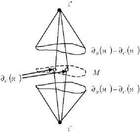
Figure 1: Causal boundary for product spacetime with $-\infty=a<b=\infty$.

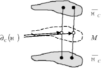
Figure 2: Causal boundary for product spacetime with $-\infty<a<b<\infty$.

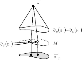
Figure 3: Causal boundary for product spacetime with $-\infty<a<b=\infty$.

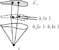
Figure 4: Causal boundary for product spacetime with $-\infty=a<b<\infty$.

4 Applications

Even though product spacetimes present a relatively simple structure, the conformal class is very general, including families of spacetimes of great interest in Relativity. Concretely, we have (standard) static spacetimes and Generalized Robertson-Walker spacetimes.

4.1 Static spacetimes

(Standard) static spacetimes can be written as

$$V={\mathbb{R}}\times M,\qquad g=-\beta(x)dt^{2}+g_{0},$$ (4.1)

where $(M,g_{0})$ is a Riemannian manifold and $\beta$ a positive function defined on $M$. A systematic study of the partial boundaries for these spacetimes was initiated by Harris in [15], and then continued in collaboration with the second author in [17]. However, these papers do not deal with the question of how to attach the partial boundaries together in order to form the (total) causal boundary. In this section we are going to apply Theorem 3.10 to cover this deficiency.

First, apply a conformal transformation to (4.1), with conformal factor $f(x)=1/\beta(x)$. We obtain the new metric

$$\overline{g}:=f(x)\cdot g=-dt^{2}+\frac{g_{0}}{\beta(x)}=-dt^{2}+h,\qquad\hbox{where}\;\;h:=g_{0}/\beta.$$

So, the conformal invariance of the causal boundary reduces the problem to study the product spacetime:

$$V={\mathbb{R}}\times M,\qquad g=-dt^{2}+h,$$

where we have renamed $\overline{g}$ by $g$. This spacetime falls under the hypothesis (i) of Theorem 3.10. Therefore:

Theorem 4.1

Let $(V,g)$ be a static spacetime as in (4.1). Assume that the spatial part $M$ endowed with metric $h=g_{0}/\beta$ falls under the hypotheses of Proposition 3.9. Then, the causal boundary (with the chronological topology) is formed by two null cones, one for the future and another for the past, with base $\partial_{B}(M)\setminus\partial_{C}(M)$ and apexes $i^{+}$ and $i^{-}$, resp., and timelike lines on each element of $\partial_{C}(M)$, with future and past extremes $i^{+}$ and $i^{-}$, resp. (Figure 1). Moreover, $\partial_{B}(M)$ is formed by two spaces $B_{\alpha}$ and $B_{\omega}$, attached at $\{\alpha\}\times K$ and $\{\omega\}\times K$, resp., with each $B_{\imath}$ ($\imath=\alpha,\omega$) being $K$ or an unique point $\ast$: $B_{\imath}\cong K$ if $|\int_{\rho_{0}}^{\imath}1/a(\rho)^{2}d\rho|<\infty$, and $B_{\imath}=\ast$ if $|\int_{\rho_{0}}^{\imath}1/a(\rho)^{2}d\rho|=\infty$. Finally, $B_{\imath}$ belongs to the Cauchy boundary $\partial_{C}(M)$ if and only if the extreme $\imath$ is finite.

Next, we are going to apply this result to some classical static spacetimes:

$\bullet$ Reissner-Nordstrom spacetime:

In local coordinates, this spacetime can be written as:

$$V={\mathbb{R}}\times(0,\infty)\times{\mathbb{S}}^{2},\qquad g=-f(r)dt^{2}+f(r)^{-1}dr^{2}+r^{2}(d\theta^{2}+\sin^{2}\theta d\phi^{2}),$$

where

$$f(r):=1-\frac{2m}{r}+\frac{q^{2}}{r^{2}}.$$

It models the gravitational field outside an electrically charged massive object which is spherically symmetric. The constants $m>0$ and $q$ can be identified with the gravitational mass and the electric charge of the object. The static regions of this spacetime are determined by condition $f(r)>0$. So, we distinguish two cases:

-Case weakly or critically charged, $|q|\leq 2m$: Here, $f(r)$ is positive for $r\in(0,r^{-})\cup(r^{+},\infty)$, where $r^{\pm}=m(1\pm\sqrt{1-(q/m)^{2}})$. First, consider the exterior region $V={\mathbb{R}}\times(r^{+},\infty)\times{\mathbb{S}}^{2}$. We have

$$M=(r^{+},\infty)\times{\mathbb{S}}^{2},\quad g_{0}=f(r)^{-1}dr^{2}+r^{2}(d\theta^{2}+\sin^{2}\theta d\phi^{2})\quad\hbox{y}\quad\beta(x)=f(r).$$

Observe that $M$ endowed with metric $h=g_{0}/\beta$ falls under the hypotheses of Proposition 3.9, being

$$(K,j_{K})=({\mathbb{S}}^{2},d\theta^{2}+\sin^{2}\theta d\phi^{2}),\quad a(\rho)=\sqrt{r^{2}/f(r)},$$

and

$$\alpha=\int^{r^{+}}_{r_{0}^{+}}1/f(r)dr=-\infty,\qquad\omega=\int_{r_{0}^{+}}^{\infty}1/f(r)dr=\infty,\qquad r^{+}_{0}\in(r^{+},\infty)$$

Moreover,

$$\left|\int_{\rho_{0}=0}^{\alpha=-\infty}\frac{1}{a(\rho)^{2}}d\rho\right|=\int_{r^{+}}^{r_{0}^{+}}\frac{dr}{r^{2}}<\infty,\qquad\left|\int_{\rho_{0}=0}^{\omega=\infty}\frac{1}{a(\rho)^{2}}d\rho\right|=\int_{r_{0}^{+}}^{\infty}\frac{dr}{r^{2}}<\infty.$$

Therefore: the causal boundary of the exterior region of weakly or critically charged Reissner-Nordstrom (with the chronological topology) is formed by two null cones at $r=r_{+}$ with base ${\mathbb{S}}^{2}$ and apexes $i^{+}$, $i^{-}$, and two null cones at infinity with base ${\mathbb{S}}^{2}$ and the same apexes $i^{+}$, $i^{-}$ (Figure 5). In particular, this is also the causal boundary for the exterior region of Schwarzschild spacetime ($q=0$).

This is in agreement with the conformal approach. The double cone at $r=r_{+}$ is due to the fact that only the region $r>r_{+}$ is considered. On the other hand, the double cone at infinity is due to the similarity between Reissner-Nordstrom and Minkowski far away from the source.

Consider now the interior region $V={\mathbb{R}}\times(0,r^{-})\times{\mathbb{S}}^{2}$. We have

$$M=(0,r^{-})\times{\mathbb{S}}^{2},\quad g_{0}=f(r)^{-1}dr^{2}+r^{2}(d\theta^{2}+\sin^{2}\theta d\phi^{2})\quad\hbox{and}\quad\beta(x)=f(r).$$

The spatial part $M$ endowed with metric $h=g_{0}/\beta$ falls again under the hypotheses of Proposition 3.9, with $(K,j_{K})$ and $a(\rho)$ as before, but now

$$\alpha=\int_{r^{-}_{0}}^{0}1/f(r)dr>-\infty,\qquad\omega=\int_{r_{0}^{-}}^{r^{-}}1/f(r)dr=\infty,\qquad r^{-}_{0}\in(0,r^{-}).$$

Moreover,

$$\left|\int_{\rho_{0}=0}^{\alpha}\frac{1}{a(\rho)^{2}}d\rho\right|=\int_{0}^{r_{0}^{-}}\frac{dr}{r^{2}}=\infty,\qquad\left|\int_{\rho_{0}=0}^{\omega=\infty}\frac{1}{a(\rho)^{2}}d\rho\right|=\int_{r_{0}^{-}}^{r^{-}}\frac{dr}{r^{2}}<\infty.$$

Therefore: the causal boundary of the interior region of weakly or critically charged Reissner-Nordstrom (with the chronological topology) is formed by two null cones at $r=r^{-}$, with base ${\mathbb{S}}^{2}$ and apexes $j^{+}$ and $j^{-}$, joined by both extremes to an unique timelike line at $r=0$, the central singularity (Figure 5).

This result justifies rigourously the identifications between the future and past timelike lines at $r=0$ suggested in [17, Sect. 6.1.3] ‘without proof’. Notice also that the Reissner-Nordstrom singularity becomes $1$-dimensional, in contraposition to the well-known ${\mathbb{R}}\times{\mathbb{S}}^{2}$ structure of the Schwarzschild singularity.

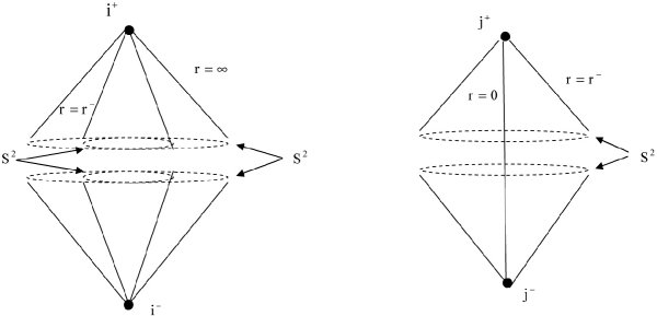
Figure 5: Causal boundary of exterior region (left picture) and interior region (right picture) of weakly or critically charged Reissner-Nordstrom.

-Case strongly charged, $|q|>2m$: Now, $f(r)>0$ for all $r$, and so, the static region coincides with the whole spacetime $V={\mathbb{R}}\times(0,\infty)\times{\mathbb{S}}^{2}$. Therefore, $M=(0,\infty)\times{\mathbb{S}}^{2}$, and $g_{0}$, $\beta$ maintain the same expression as before. The spatial part $M$ endowed with metric $h=g_{0}/\beta$ falls under the hypotheses of Proposition 3.9, being $(K,j_{K})$ and $a(\rho)$ as in previous cases, and

$$\alpha=\int^{0}_{r_{0}}1/f(r)dr>-\infty,\qquad\omega=\int_{r_{0}}^{\infty}1/f(r)dr=\infty.$$

Moreover,

$$\left|\int_{\rho_{0}=0}^{\alpha}\frac{1}{a(\rho)^{2}}d\rho\right|=\int_{0}^{r_{0}}\frac{dr}{r^{2}}=\infty,\qquad\left|\int_{\rho_{0}=0}^{\omega=\infty}\frac{1}{a(\rho)^{2}}d\rho\right|=\int_{r_{0}}^{\infty}\frac{dr}{r^{2}}<\infty.$$

Therefore: the causal boundary of strongly charged Reissner-Nordstrom (with the chronological topology) is formed by two null cones at $r=\infty$ with base ${\mathbb{S}}^{2}$ and apexes $i^{+}$, $i^{-}$, and a timelike line at $r=0$ with the same extremes $i^{+}$, $i^{-}$. (In this case, the diagram corresponds to the right picture in Figure 5 with $r^{-}=\infty$ and $j^{+},j^{-}$ replaced by $i^{+},i^{-}$.)

$\bullet$ Anti-de Sitter spacetime:

This spacetime of constant sectional curvature $-1$ and topology ${\mathbb{S}}^{1}\times{\mathbb{R}}^{3}$ does contain closed timelike curves. In particular, it is not strongly causal, and thus, the causal boundary approach cannot apply. However, this spacetime is not $1$-connected, being its universal cover strongly causal and static. Consequently, in this section by Anti-de Sitter spacetime we will understand its universal cover.

In local coordinates, Anti-de Sitter spacetime can be written as

$$V={\mathbb{R}}\times(0,\infty)\times{\mathbb{S}}^{2},\qquad g=-\cosh^{2}(r)dt^{2}+dr^{2}+\sinh^{2}(r)(d\theta^{2}+\sin^{2}\theta d\phi^{2}).$$

According to the notation previously introduced, we have

$$M=(0,\infty)\times{\mathbb{S}}^{2},\quad g_{0}=dr^{2}+\sinh^{2}(r)(d\theta^{2}+\sin^{2}\theta d\phi^{2})\quad\hbox{y}\quad\beta(x)=\cosh^{2}(r).$$

The spatial part $M$ endowed with metric $h=g_{0}/\beta$ falls under the hypotheses of Proposition 3.9, being

$$(K,j_{K})=({\mathbb{S}}^{2},d\theta^{2}+\sin^{2}\theta d\phi^{2}),\quad a(\rho)=\tanh(r),$$

and

$$\alpha=\int_{r_{0}=1}^{0}\frac{dr}{\beta(x)}=\int_{1}^{0}\frac{dr}{\cosh(r)}>-\infty,\qquad\omega=\int_{r_{0}=1}^{\infty}\frac{dr}{\beta(x)}=\int_{1}^{\infty}\frac{dr}{\cosh(r)}dr<\infty.$$

Moreover,

$$\left|\int^{\alpha}_{\rho_{0}=0}\frac{1}{a(\rho)^{2}}d\rho\right|=\int_{0}^{1}\frac{\cosh(r)}{\sinh^{2}(r)}dr=\infty,\quad\left|\int_{\rho_{0}=0}^{\omega}\frac{1}{a(\rho)^{2}}d\rho\right|=\int_{1}^{\infty}\frac{\cosh(r)}{\sinh^{2}(r)}dr<\infty.$$

Therefore, if we ignore the boundary region associated to $r=0$, which is not representative because it corresponds to a coordinate singularity, we obtain the following structure: the causal boundary of Anti-de Sitter spacetime (with the chronological topology) is formed just by a timelike surface at $r=\infty$ of section ${\mathbb{S}}^{2}$, which connects the points $i^{+}$ and $i^{-}$ (Figure 6).

In particular, this structure coincides with the conformal boundary. Notice however that points $i^{+}$, $i^{-}$ are isolated in the conformal approach [18, p. 132].

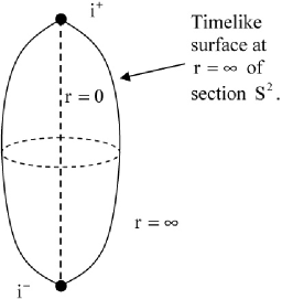
Figure 6: Causal boundary of Anti-de Sitter spacetime.

$\bullet$ Taub spacetime:

This spacetime, firstly introduced by A. H. Taub in [19], can be written as:

$$V={\mathbb{R}}^{3}\times(0,\infty),\qquad g=\rho^{-1/2}(-dt^{2}+d\rho^{2})+\rho(dx^{2}+dy^{2}),\;\;(\rho>0).$$

It is the unique solution of empty Einstein equations without cosmological term, which is plane symmetric and static. The causal boundary of Taub spacetime was studied by Kuang, Li and Liang in [8]. Surprisingly, they found that the singular region of the boundary reduces to one point when the GKP construction is applied, in contraposition to the $1$-dimensional structure physically expected. Since then, this result has been claimed as an important evidence that GKP approach is not totally satisfactory. Next, we are going to apply Theorem 4.1 in order to show that this defect is not present in the approach followed in this paper.

According to the notation previously introduced, now we have:

$$M=(0,\infty)\times{\mathbb{R}}^{2},\quad g_{0}=\rho^{-1/2}d\rho^{2}+\rho dx^{2}+\rho dy^{2}\quad\hbox{y}\quad\beta(x)=\rho^{-1/2}.$$

Therefore,

$$(K,j_{K})=({\mathbb{R}}^{2},dx^{2}+dy^{2}),\quad(\alpha,\omega)=(0,\infty)\quad\hbox{y}\quad a(\rho)=\rho^{3/2}.$$

In this case, the spatial part $M$ endowed with metric $h=g_{0}/\beta$ does not fall under the hypotheses of Proposition 3.9, since $K={\mathbb{R}}^{2}$ is not compact. However, from the analysis and classification of the pasts and futures of inextensible causal curves developed in [8, pp. 1534-5], it implicitly follows

$$\partial_{B}(M)=B_{\alpha=0}\cup B_{\omega=\infty},\quad\hbox{being}\;\;B_{0}=*,\;\;B_{\infty}={\mathbb{R}}^{2}.$$

Therefore, from the first part of Theorem 4.1 (recall Remark 3.11), we obtain: the causal boundary of Taub spacetime is formed by a timelike line at $\rho=0$ of future and past extremes $i^{+}$, $i^{-}$, resp., and two null cones at $\rho=\infty$, one for the future and another for the past, with base ${\mathbb{R}}^{2}$ and apexes $i^{+}$, $i^{-}$, resp. (Figure 7).

In conclusion, this result does reproduce the $1$-dimensional character of the Taub singularity, represented by the region of the boundary at $\rho=0$.

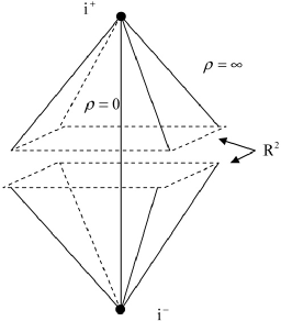
Figure 7: Causal boundary of Taub spacetime.

4.2 Generalized Robertson-Walker spacetimes

By Generalized Robertson-Walker (GRW) spacetimes we understand the family of spacetimes given by:

$$V=(a^{\prime},b^{\prime})\times M,\qquad g=-dt^{2}+\alpha(t)h,$$ (4.2)

where $(a^{\prime},b^{\prime})\subseteq{\mathbb{R}}$ is an open interval of ${\mathbb{R}}$ called base, $(M,h)$ is an arbitrary Riemannian manifold called fiber and $\alpha(t)$ is a positive function defined on $(a^{\prime},b^{\prime})$ called warping function or scale factor. This family is quite important in Relativity, since it provides a first approach to the global structure of the universe: not for nothing it arises as a natural generalization of the standard cosmological models (studied in a moment). See [20, 21] for local and global geometrical characterizations of GRW spacetimes.

The causal boundary of these spacetimes can be obtained by applying the result [13, Proposition 5.2], which describes the partial boundaries for the more general family of multiwarped spacetimes (i.e., multiple fibers and multiple warping functions considered). However, this result does not work when the resulting boundary has non-spacelike regions. In this section we are going to use Theorem 3.10 to extend this result to cover any causal character for the boundary, at least in the smaller class of GRW spacetimes.

To this aim, first apply a conformal transformation to (4.2), with conformal factor $f(t)=1/\alpha(t)$. We obtain the new metric

$$\overline{g}:=f(t)\cdot g=-\frac{dt^{2}}{\alpha(t)}+h=-ds^{2}+h,$$

where the variable $s$ is defined by the relation $ds=dt/\sqrt{\alpha(t)}$. Taking into account the conformal invariance of the causal boundary, we only need to study the product spacetime

$$V=(a,b)\times M,\qquad\overline{g}=-ds^{2}+h,$$

where $I=(a,b)$ is the domain for the new variable $s$, and thus, it may be different from the initial interval $(a^{\prime},b^{\prime})$. From the relation between $s$ and $t$ it directly follows:

$$a=-\int^{c_{0}}_{a^{\prime}}\frac{1}{\sqrt{\alpha(t)}}dt,\qquad b=\int^{b^{\prime}}_{c_{0}}\frac{1}{\sqrt{\alpha(t)}}dt,\qquad a^{\prime}<c_{0}<b^{\prime}.$$

Therefore, we conclude that the causal boundary of GRW spacetime (4.2) coincides with that of the spacetime

$$V=I\times M,\qquad g=-dt^{2}+h,$$ (4.3)

where we have renamed $\overline{g}$ and $s$ by $g$ and $t$, resp. Theorem 3.10 applied to (4.3) then provides the following result:

Theorem 4.2

Let $V=(a^{\prime},b^{\prime})\times M$, $g=-dt^{2}+\alpha(t)h$ be a GRW spacetime with spatial part $(M,h)$ under the hypotheses of Proposition 3.9. Then, the causal boundary (with the chronological topology) has the following structure:

• If $\int_{a^{\prime}}^{c_{0}}1/\sqrt{\alpha(t)}dt=\int^{b^{\prime}}_{c_{0}}1/\sqrt{\alpha(t)}dt=\infty$ then it is formed by two infinity null cones, one for the future and another for the past, with base $\partial_{B}(M)\setminus\partial_{C}(M)$ and apexes $i^{+}$ and $i^{-}$, resp., and timelike lines of future and past extremes $i^{+}$ and $i^{-}$, resp., on each point of $\partial_{C}(M)$ (Figure 1).

• If $\int_{a^{\prime}}^{c_{0}}1/\sqrt{\alpha(t)}dt,\,\int^{b^{\prime}}_{c_{0}}1/\sqrt{\alpha(t)}dt<\infty$ then it is formed by two copies, one for the future and another for the past, of the Cauchy completion $\overline{M}_{C}$ of $(M,h)$, and timelike lines based on each point of $\partial_{C}(M)$ which connect both copies (Figure 2).

• If $\int_{a^{\prime}}^{c_{0}}1/\sqrt{\alpha(t)}dt<\infty$, $\int^{b^{\prime}}_{c_{0}}1/\sqrt{\alpha(t)}dt=\infty$ then it is formed by an infinity null cone for the future with base $\partial_{B}(M)\setminus\partial_{C}(M)$ and apex $i^{+}$, a copy of $\overline{M}_{C}$ for the past, and timelike lines based on each point of $\partial_{C}(M)$ which connect $\overline{M}_{C}$ with $i^{+}$ (Figure 3).

• If $\int_{a^{\prime}}^{c_{0}}1/\sqrt{\alpha(t)}dt=\infty$, $\int^{b^{\prime}}_{c_{0}}1/\sqrt{\alpha(t)}dt<\infty$ then it is formed by an infinity null cone for the past with base $\partial_{B}(M)\setminus\partial_{C}(M)$ and apex $i^{-}$, a copy of $\overline{M}_{C}$ for the future, and timelike lines based on each point of $\partial_{C}(M)$ which connect $i^{-}$ with $\overline{M}_{C}$ (Figure 4).

Moreover, $\partial_{B}(M)$ is formed by two spaces $B_{\alpha}$ and $B_{\omega}$, attached at $\{\alpha\}\times K$ and $\{\omega\}\times K$, resp., with each $B_{\imath}$ ($\imath=\alpha,\omega$) being $K$ or an unique point $\ast$: concretely, $B_{\imath}\cong K$ if $|\int_{\rho_{0}}^{\imath}1/a(\rho)^{2}d\rho|<\infty$, and $B_{\imath}=\ast$ if $|\int_{\rho_{0}}^{\imath}1/a(\rho)^{2}d\rho|=\infty$. Finally, $B_{\imath}$ belongs to the Cauchy boundary $\partial_{C}(M)$ if and only if the extreme $\imath$ is finite.

In particular, the structure of the causal boundary for GRW spacetimes depends on both, the spatial part $(M,h)$ and the scale factor $\alpha(t)$. If the spatial part $(M,h)$ is complete ($\partial_{C}(M)=\emptyset$), the boundary presents at each extreme of the temporal interval $(a^{\prime},b^{\prime})$, either a spacelike cover structure $M$ or a null cone with base $\partial_{B}(M)$, depending on the growth of the scale factor at each extreme. However, if the spatial part $(M,h)$ is incomplete ($\partial_{C}(M)\neq\emptyset$), the boundary will also contain timelike lines on each point of $\partial_{C}(M)$, reachable by observers of the universe in finite proper time. Hence, the boundary is not necessarily time symmetric and may contain regions of any causal character (null, timelike or spacelike).

$\bullet$ FLRW spacetimes:

By completeness, we are going to particularize previous result to Friedman-Lemaitre-Robertson-Walker (FLRW) spacetimes, i.e. the spatial part is now a geometric model. In this case, the spacetime manifold $V_{k}$ is either $(a^{\prime},b^{\prime})\times{\mathbb{R}}^{3}$ if $k=0,-1$ or $(a^{\prime},b^{\prime})\times{\mathbb{S}}^{3}$ if $k=1$. In local coordinates, the line element reads

$$g=-dt^{2}+\alpha(t)[d\rho^{2}+a(\rho,k)^{2}(d\theta^{2}+\sin^{2}\theta d\phi^{2})],$$

where $\alpha(t)$ is the scale factor and

$$a(\rho,k)=\left\{\begin{array}[]{ll}\sin\rho&\hbox{if}\;\;k=1\\ \rho&\hbox{if}\;\;k=0\\ \sinh\rho&\hbox{if}\;\;k=-1.\end{array}\right.$$

Therefore, Theorem 4.2 gives:

Theorem 4.3

The causal boundary of a FLRW spacetime, $V=(a^{\prime},b^{\prime})\times M$, $g=-dt^{2}+\alpha(t)h$ with $(M,h)\equiv{\mathbb{R}}^{3},{\mathbb{S}}^{3}$ or $\hbox{\ddpp H}^{3}$, has the following structure:

• If $\int_{a^{\prime}}^{c_{0}}1/\sqrt{\alpha(t)}dt=\int^{b^{\prime}}_{c_{0}}1/\sqrt{\alpha(t)}dt=\infty$ then it is formed by two infinity null cones, one for the future and another for the past, with base ${\mathbb{S}}^{2}$ and apex $i^{+}$ and $i^{-}$, resp., if $M={\mathbb{R}}^{3},\hbox{\ddpp H}^{3}$, or it is formed just by $i^{+}$, $i^{-}$ if $M={\mathbb{S}}^{3}$.

• If $\int_{a^{\prime}}^{c_{0}}1/\sqrt{\alpha(t)}dt,\,\int^{b^{\prime}}_{c_{0}}1/\sqrt{\alpha(t)}dt<\infty$ then it is formed by two spacelike copies, one for the future and another for the past, of ${\mathbb{R}}^{3}$ if $M={\mathbb{R}}^{3},\hbox{\ddpp H}^{3}$, or ${\mathbb{S}}^{3}$ if $M={\mathbb{S}}^{3}$.

• If $\int_{a^{\prime}}^{c_{0}}1/\sqrt{\alpha(t)}dt<\infty$, $\int^{b^{\prime}}_{c_{0}}1/\sqrt{\alpha(t)}dt=\infty$ then it is formed by an infinity null cone for the future with base ${\mathbb{S}}^{2}$ and apex $i^{+}$ and a copy of ${\mathbb{R}}^{3}$ for the past if $M={\mathbb{R}}^{3},\hbox{\ddpp H}^{3}$, or it is formed by $i^{+}$ for the future and a copy of ${\mathbb{S}}^{3}$ for the past if $M={\mathbb{S}}^{3}$.

• If $\int_{a^{\prime}}^{c_{0}}1/\sqrt{\alpha(t)}dt=\infty$, $\int^{b^{\prime}}_{c_{0}}1/\sqrt{\alpha(t)}dt<\infty$ then it is formed by an infinity null cone with base ${\mathbb{S}}^{2}$ and apex $i^{-}$ and a copy of ${\mathbb{R}}^{3}$ for the future if $M={\mathbb{R}}^{3},\hbox{\ddpp H}^{3}$, or it is formed by $i^{-}$ for the past and a copy of ${\mathbb{S}}^{3}$ for the future if $M={\mathbb{S}}^{3}$.

Proof. If $k=0,-1$, the spatial part is

$$M=(0,\infty)\times{\mathbb{S}}^{2},\quad h=d\rho^{2}+a(\rho,k)^{2}(d\theta^{2}+\sin^{2}\theta d\phi^{2}),\;\;a(\rho,k)=\left\{\begin{array}[]{ll}\rho&\hbox{if}\;\;k=0\\ \sinh\rho&\hbox{if}\;\;k=-1.\end{array}\right.$$

In particular, $(M,h)$ falls under the hypotheses of Proposition 3.9. Therefore, the conclusion directly follows from Theorem 4.2 and the integrals

$$\left|\int^{0}_{\rho_{0}=1}\frac{1}{a(\rho,k)^{2}}d\rho\right|=\infty,\qquad\left|\int_{\rho_{0}=1}^{\infty}\frac{1}{a(\rho,k)^{2}}d\rho\right|<\infty.$$

(Obviously, we have ignored the boundary region at $\rho=0$.)

Assume now that $k=1$. In this case, $a(\rho,1)=\sin\rho$, and thus, the spatial part does not fall under the hypotheses of Proposition 3.9. However, from Remark 3.11 the first part of Theorem 4.2 still holds. Whence, the conclusion directly follows from $\partial_{B}({\mathbb{S}}^{3})=\partial_{C}({\mathbb{S}}^{3})=\emptyset$ and $\overline{M}_{C}=M={\mathbb{S}}^{3}$. $\Box$

An immediate application of this result gives the causal boundary for Einstein Static Universe. This spacetime is a FLRW model with base ${\mathbb{R}}$, fiber $(M,h)\equiv{\mathbb{S}}^{3}$ and scale factor $\alpha(t)\equiv 1$. Therefore, taking into account that $\int_{-\infty}^{0}dt=\int^{\infty}_{0}dt=\infty$: the causal boundary of ESU is formed by the points, $i^{+}$, $i^{-}$. In this case, the weak (indeed, null) asymptotic growth of the scale factor implies degeneration of the boundary in two unique points. On the opposite side we have de Sitter spacetime. This is a FLRW model with base ${\mathbb{R}}$, fiber $(M,h)\equiv{\mathbb{S}}^{3}$ and scale factor $\alpha(t)=\cosh(t)$. Therefore, taking into account that $\int_{-\infty}^{0}1/\cosh(t)dt=\int_{0}^{\infty}1/\cosh(t)dt<\infty$: the causal boundary of de Sitter spacetime is formed by two spacelike copies of ${\mathbb{S}}^{3}$, one for the past and another for the future. So, it is the strong asymptotic growth of the scale factor $\alpha(t)=\cosh(t)$ which produces this big boundary.

5 Conclusions

The main result in this paper is Theorem 3.10, which describes the causal boundary for product spacetimes of a Lorentz interval and a Riemannian manifold. The huge conformal class of these spacetimes, which includes both, (standard) static spacetimes and Generalized Robertson-Walker spacetimes, makes this result specially useful to deduce the boundary of multiple classical spacetimes. In particular, we have explicitly described the causal boundary for Reissner-Nordstrom (including Schwarzschild), Anti-de Sitter, Taub and standard cosmological models as de Sitter spacetime and Einstein Static Universe.

In this paper we have used the formulation of the causal boundary introduced in [1], and modified later in [2]. As consequence, we have tested this new formulation for the classical spacetimes previously cited. In particular, we have found that the causal boundary essentially reproduces the structure of the conformal boundary in these cases: right identifications between the temporal lines of the boundary, expected dimensionality for the singular regions, satisfactory topology for the completion…

This paper can be considered a very initial step in the ambitious project of describing the causal boundary of spacetimes $V=I\times M$ with metric $g=-dt^{2}+h_{t}$, where $h_{t}$ may depend on time. As an indication of the importance and generality of this problem, just recall that any globally hyperbolic spacetime admits this decomposition, see [22]. Another step within this program may consist of completing the results about the boundary of multiwarped spacetimes in [13]. These spacetimes are very interesting because, apart from including certain regions of Schwarzschild and Reissner-Nordstrom uncovered in this paper, they also include Bianchi type IX spacetimes (as Kasner), spacetimes with internal degrees of freedom attached at every point and multidimensional inflationary models.

References

- [1] D. Marolf, S.R. Ross, Class. Quant. Grav., 20 (2003) 4085.
- [2] J.L. Flores, The Causal Boundary of spacetimes revisited. Preprint (2006). Available at gr-qc/0608063.
- [3] R. Penrose, Relativity, Groups and Topology, ed. C.M. de Witt and B. de Witt, (1964, Gordon and Breach, New York); Proc. Roy. Soc. Lond. A 284 (1965), 159.
- [4] R.P. Geroch, E.H. Kronheimer, R. Penrose, Proc. Roy. Soc. Lond. A 237 (1972), 545.
- [5] R. Budic, R.K. Sachs, J. Math. Phys. 15 (1974), 1302.
- [6] I. Racz, Phys. Rev. D 36 (1987), 1673; Gen. Relat. Grav. 20 (1988), 893.
- [7] L.B. Szabados, Class. Quant. Grav. 5 (1988), 121; Class Quant. Grav. 6 (1989), 77.
- [8] Kuang zhi-quan, Li jian-zeng and Liang can-bi, Phys. Rev. D 33 (1986), 1533.
- [9] Kuang zhi-quan, Liang can-bi, J. Math. Phys. 29 (1988), 433.
- [10] Kuang zhi-quan, Liang can-bi, Phys. Rev. D 46 (1992), 4253.
- [11] A. G -Parrado, J.M.M. Senovilla, Class. Quant. Grav. 22 (2005) R1.
- [12] S. Harris, Contemp. Math., 359 (2004), 65.
- [13] S. Harris, Class. Quant. Grav., 17 (2000), 551.
- [14] J.L. Flores, M. Sánchez, Causal Boundary for general plane waves. In progress.
- [15] S. Harris, Nonlinear Anal., 47 (2001), 2971.
- [16] J.K. Beem, P.E. Ehrlich, K.L. Easley, Global Lorentzian geometry, Monographs Textbooks Pure Appl. Math. 202 (Dekker Inc., New York, 1996).
- [17] J.L. Flores, S. Harris, Class. Quant. Grav. 24 (2007), 1211.
- [18] S.W. Hawking, G.F.R. Ellis, The Large Scale Structure of Space-Time, Cambridge University, Cambridge, 1973.
- [19] A.H. Taub, Ann. Math. 53 (1951), 472.
- [20] M. Sánchez, Gen. Relat. Grav. 30 (1998), 915.
- [21] M. Gutierrez, B. Oleá, Global decomposition of a Lorentzian manifold as a Generalized Robertson-Walker space. Preprint (2007). Available at math/0701067.
- [22] A. Bernal, M. Sánchez, Comm. Math. Phys. 243 (2003), 461; Comm. Math. Phys. 257 (2005), 43.