Ab initio theory of helix$\leftrightarrow$coil phase transition

Abstract

In this paper we suggest a theoretical method based on the statistical mechanics for treating the $\alpha$-helix$\leftrightarrow$random coil transition in alanine polypeptides. We consider this process as a first-order phase transition and develop a theory which is free of model parameters and is based solely on fundamental physical principles. It describes essential thermodynamical properties of the system such as heat capacity, the phase transition temperature and others from the analysis of the polypeptide potential energy surface calculated as a function of two dihedral angles, responsible for the polypeptide twisting. The suggested theory is general and with some modification can be applied for the description of phase transitions in other complex molecular systems (e.g. proteins, DNA, nanotubes, atomic clusters, fullerenes).

I Introduction

The phase transitions in finite complex molecular systems, i.e. the transition from a stable 3D molecular structure to a random coil state or vice versa (also known as (un)folding process), has a long standing history of investigation (for review see, e.g. Shakhnovich (2006); Finkelstein and Ptitsyn (2002); Shea and Brooks (2001); Prabhu and Sharp (2005)). The phase transitions of this or similar nature occur or can be expected in many different complex molecular systems and in nano objects, such as polypeptides, proteins, polymers, DNA, fullerenes, nanotubes Yakubovich et al. (2007a). They can be understood as first order phase transitions, which are characterized by rapid growth of the system’s internal energy at a certain temperature. As a result, the heat capacity of the system as a function of temperature acquires a sharp maximum at the temperature of the phase transition.

In our recent paper Yakubovich et al. (2006a) a novel ab initio theoretical method for the description of phase transitions in the mentioned molecular systems has been suggested. In particular, it was demonstrated that in polypeptides (chains of amino acids) one can identify specific, so-called twisting degrees of freedom responsible for the folding dynamics of amino acid chains, i.e. for the transition from a random coil state of the chain to its $\alpha$-helix structure. The twisting degrees of freedom are also sometimes referred as the torsion degrees of freedom. The essential domain of the potential energy surface of polypeptides with respect to these twisting degrees of freedom can be calculated and thoroughly analyzed on the basis of ab initio methods such as density functional theory (DFT) or Hartree-Fock method. It was shown Yakubovich et al. (2006a) that this knowledge is sufficient for the construction of the partition function of a polypeptide chain and thus for the development of its complete thermodynamic description, which includes the calculation of all essential thermodynamic variables and characteristics, e.g. free energy, heat capacity, phase transition temperature, etc. The method has been proved to be applicable for the description of the phase transition in polyalanine chains of different lengths by the comparison of the theory predictions with the results of several independent experiments and of molecular dynamics simulations. Similar descriptions can be developed for a large variety of complex molecular systems.

Earlier studies of the folding process based on the statistical mechanics principles (see Zimm and Bragg (1959); Gibbs and DiMarzio (1959); Lifson and Roig (1961); Schellman (1958)) always contained some empirical parameters and thus could hardly be used for ab initio predictions of essential characteristics of the phase transitions. Since then, the total number of papers devoted to this problem is very large. Here we do not intend to review all of them, but refer in this article only to those, which are related directly to our work (for review see also Shakhnovich (2006); Shea and Brooks (2001); Prabhu and Sharp (2005) and references therein).

The first theoretical attempt to describe the folding process of polypeptides was done by Zimm and Bragg Zimm and Bragg (1959). In their work the process of polypeptide $\alpha$-helix formation was considered within the framework of simple two-state statistical model. This model contains three principal parameters: (i) a constant describing the probability of an amino acid to bond in the helix conformation to a part of the chain being in the helical form, (ii) a special correction factor for the initiation of helix formation (i.e. a factor describing the probability of an amino acid to bond in the helix conformation to an amino acid that is in the random coil state), and (iii) the minimum number of amino acids allowed to exist in the random coil state between two helical parts.

A different set of parameters was suggested in Gibbs and DiMarzio (1959). The major parameters used in that paper are the energies of hydrogen bonds in the polypeptide chain and the number of possible conformations in the random coil state. These two parameters define the energy and entropy differences between folded and unfolded states of the polypeptide. In Schellman (1958) the factors affecting the stability of polypeptide structures in solution were discussed.

In Lifson and Roig (1961) the partition function of a polypeptide chain was determined as a function of generalized coordinates corresponding to the twisting degrees of freedom of the molecule’s backbone. In that paper the conditional probabilities of the occurrence of helical and coil states of the peptide units are obtained in the form of a $3\times 3$ matrix. The eigenvalues of this matrix yield the various molecular averages as functions of the degree of polymerization, temperature, and molecular constants. The theoretical model suggested in Lifson and Roig (1961) contained three parameters which describe the statistical weights of three possible states of an amino acid in a polypeptide chain: the helix state, the coil state and the boundary state occurring at the interface between the helix and the coil phases.

In Lifson (1964) another method was suggested for the derivation of the partition function of linear-chain molecules. The partition function was constructed on the basis of the so-called defining sequences, being a sequence of numbers that describe the lengths of the polypeptide parts found in different conformational states. Therefore the defining sequence describes a certain microstate of the system. The partition function of the system was constructed from the partition functions of the defining sequences. To do so, some special functions were introduced, which are called as the sequence-generating functions. The method suggested in Lifson (1964) was used in Poland and Scheraga (1966a) for the study of helix-coil transition in polypeptides. In that paper the conditions for the occurrence of phase transition in one dimensional system were analyzed. In Poland and Scheraga (1966b) the kinetics of helix-coil transition was studied within the theoretical frameworks developed in Lifson and Roig (1961); Lifson (1964).

In Go and Scheraga (1976, 1969) the importance of various internal degrees of freedom in polypeptide was discussed. The partition function of the system was constructed within the framework of classical and quantum mechanics.

The helix-coil transition of polypeptides was also studied in Refs. Ooi and Oobatake (1991); Gomez et al. (1995). In those papers general equations of statistical physics were used to describe this transition. Those theories contained several parameters (such as enthalpy, entropy, free energy changes) which were fitted to represent results of independent experimental observations.

The molecular dynamics (MD) approach, an alternative to using statistical physics, has been widely used during the last decade for studying structural transitions in polypeptides. Full atomistic molecular dynamics Tobias and Brooks (1991); Garcia and Sanbonmatsu (2002); Nymeyer and Garcia (2003) and Monte-Carlo based techniques Irbäck and Sjunnesson (2004); Shental-Bechor et al. (2005) were used for studying alanine tripeptide Tobias and Brooks (1991), alanine pentapeptide Garcia and Sanbonmatsu (2002) and alanine 21-peptide Nymeyer and Garcia (2003); Shental-Bechor et al. (2005). The molecular dynamics simulations were carried out within the framework of classical mechanics with an empirical Hamiltonian usually referred as the forcefield. The most popular forcefields developed during recent years are GROMOS Scott and van Gunsteren (1995), AMBER Cornell et al. (1995) and CHARMM MacKerell. et al. (1998).

During the last years molecular dynamics was also widely applied for studying the folding process of small proteins Chen et al. (2005); Duan and Kollman (1998); Liwo et al. (2005); Ding et al. (2002); Pande et al. (2002); Irbäck et al. (2003). Such simulations became possible relatively recently due to modern computer powers. However, it is still not feasible to perform molecular dynamics simulations of the folding process of large proteins Shakhnovich (2006) because the characteristic timescale of this process varies from micro seconds to minutes Kubelka et al. (2004); Lipman et al. (2003), being several orders of magnitude larger than the time of possible molecular dynamics simulations.

Another molecular dynamics approach for studying the protein folding problem was suggested in He and Scheraga (1998a, b). In these papers the dynamics of the macromolecule was considered in the phase space of torsional degrees of freedom.

Stochastic treatment of helix-coil transition in polypeptides was performed in Fujita et al. (1981); Cárdenas and Elber (2003). In Fujita et al. (1981) the application of correlated random walk theory for polypeptides was analyzed. In Cárdenas and Elber (2003) an atomistic simulation of helix formation with the stochastic difference equation was performed.

The helix-coil transition of polypeptides has also been extensively studied experimentally Scholtz et al. (1991); Lednev et al. (2001); Thompson et al. (1997); Williams et al. (1996). In Scholtz et al. (1991) the enthalpy change accompanying the $\alpha$-helix to coil transition has been determined calorimetrically for a 50-residue Ac-Y(AEAAKA)₈F-NH₂ peptide that contains primarily alanine. The dependence of the heat capacity of the polypeptide on temperature was measured with the use of differential scanning calorimetry method. In Lednev et al. (2001); Thompson et al. (1997) the experiments were performed for A₅(A₃RA)₃A and MABA-A₅-(AAARA)₃-A-NH₂ alanine-rich peptides consisting of $21$ amino acids by means of UV resonance Raman spectroscopy and by circular dichroism, respectively. The dependence of helicity on temperature was recorded. Kinetics of the helix-coil transition of 21 residue Suc-AAAAA-(AAARA)₃A-NH₂ alanine based polypeptide was studied in Williams et al. (1996) by means of infrared spectroscopy.

Previous attempts to describe the helix-coil transition in polypeptide chains within the framework of statistical physics were based on the models suggested in the sixties Zimm and Bragg (1959); Gibbs and DiMarzio (1959); Lifson and Roig (1961); Schellman (1958), where the general formalism for the construction of the partition function of polypeptides was suggested. Earlier theories always included several parameters in the partition function making it parameter dependent. The methods suggested in Zimm and Bragg (1959); Gibbs and DiMarzio (1959); Lifson and Roig (1961); Schellman (1958) were widely used for the description of the helix-coil transition in polypeptide chains (see Refs. Kromhout and Linder (2001); Chakrabartty et al. (1994); Shakhnovich (2006); Finkelstein and Ptitsyn (2002); Shea and Brooks (2001); Go et al. (1970); Scheraga et al. (2002); Shental-Bechor et al. (2005)). The dependance of the thermodynamic characteristics of the $\alpha$-helix$\leftrightarrow$random coil phase transition in polypeptides on model parameters, used for the partition function construction, was thoroughly analysed (see papers cited above). Some attempts were made to obtain these parameters from experimental observations and from the theoretical calculations. In Wójcik et al. (1990) the parameters of the Zimm and Bragg theory Zimm and Bragg (1959) were deduced from the optical rotatory dispersion and circular dichroism measurements on poly(L-cystine) in water at neutral pH.

The first attempts to evaluate the parameters of the Zimm-Bragg theory theoretically were performed in Go et al. (1970). In that paper a semi-empirical potential Scott and Scheraga (1966); Ooi et al. (1967) was used to describe the conformational dynamics of the polypeptide. The potential suggested in these papers is similar to the modern forcefields Scott and van Gunsteren (1995); Cornell et al. (1995); MacKerell. et al. (1998), but treats the structure of a polypeptide in a simplified way by neglecting some of the hydrogen atoms in the polypeptide and making minimal assumptions about the hybridization of atoms. The potential used in Scott and Scheraga (1966); Ooi et al. (1967) can be considered as one of the first (if not the first) forcefields suggested. With its use in Go et al. (1970) the parameters of the Zimm-Bragg theory were calculated and the temperature of the helix-coil transition in polypeptide chain was established. In that paper the partition function was constructed and evaluated within a matrix approach developed in Lifson and Roig (1961)

The parameters of the Zimm-Bragg theory were also calculated by means of molecular dynamics simulation Wang et al. (1995). A peptide growth simulation method was introduced, which allowed the generation of dynamic models of polypeptide chains in $\alpha$- helix or random coil conformations. With this method the Zimm-Bragg parameters for helix initiation and helix growth have been calculated.

In the present paper we describe an alternative theoretical approach based on the statistical mechanics for treating the $\alpha$-helix$\leftrightarrow$random coil phase transition in alanine polypeptides. The suggested method is a further development of the method suggested in Yakubovich et al. (2006a, 2007a), which is based on the construction of a parameter-free partition function for a system experiencing a phase transition. All the necessary information for the construction of such a partition function can be calculated on the basis of ab initio DFT, combined with molecular mechanics theories. Comparison of the results of this method with the results of molecular dynamics simulations (see following paper Yakubovich et al. (2007b)) allows one to establish the accuracy of the new approach for sufficiently large molecular systems and then to extend the description to the larger molecular objects, which is especially essential in those cases when molecular dynamics simulations are hardly possible because of computer power limitations.

We note that the suggested method is considered as an efficient novel alternative to the existing theoretical approaches for the study of helix-coil transitions in polypeptides since it does not contain any model parameters and gives a universal recipe for the construction of the partition function in complex molecular systems. The partition function of the polypeptide is constructed based on a minimal number of assumptions about the system which are different from those used in earlier theories. It includes all essential physical contributions needed for the description of the helix-coil transition in polypeptides. Therefore the final expression for the partition function obtained within the framework of our theory is different from the ones suggested earlier.

In this paper we present in detail the theoretical method for the study of $\alpha$-helix$\leftrightarrow$random coil phase transitions in polypeptides, while in the following paper Yakubovich et al. (2007b) we report the results of numerical simulations of this process.

II Statistical model for the $\alpha$-helix$\leftrightarrow$random coil phase transition

Let us consider a polypeptide, consisting of $n$ amino acids. The polypeptide can be found in one of its numerous isomeric states that have different energies. A group of isomeric states with similar characteristic physical properties is called a phase state of the polypeptide. Thus, a regular bounded $\alpha$-helix state corresponds to one phase state of the polypeptide, while all possible unbounded random conformations can be denoted as the random coil phase state.

The phase transition is the transformation of the polypeptide from one phase state to another, i.e. the transition from a regular $\alpha$-helix conformation to a group of unbounded random conformations. The characteristic structural change of alanine polypeptide experiencing an $\alpha$-helix$\leftrightarrow$random coil phase transition is shown in Fig. 1. In this figure we show only one characteristic conformation of the polypeptide in the random coil state, while there exist about $10^{30}$ different conformations of 21 alanine polypeptide (see Yakubovich et al. (2006a) for more details).

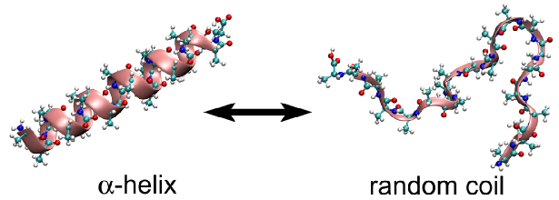
Figure 1: The characteristic structural change of alanine polypeptide experiencing an $\alpha$-helix$\leftrightarrow$random coil phase transition.

The phase transition can either be of the first or of the second order. The first order phase transition is characterized by an abrupt change of the internal energy of the system with respect to its temperature. In the first order phase transition the system either absorbs or releases a fixed amount of energy while the heat capacity as a function of temperature has a pronounced peak Finkelstein and Ptitsyn (2002). We study the manifestation of these features for alanine polypeptide chains of different lengths.

II.1 Hamiltonian of a polypeptide chain

To study thermodynamic properties of the system one needs to investigate its potential energy surface with respect to all degrees of freedom. There are a number of different methods for calculating the energy of many-body systems. The most accurate approaches are based on solving the Schrödinger equation. These approaches are usually referred as ab initio methods since they involve a minimum number of assumptions about the system.

For complex molecular systems ab initio calculations require significant computer power. Depending on the method, the computational cost of such calculations grows as $N^{2}$ or even $N^{8}$ Foresman and leen Frisch (1996), where $N$ is the number of particles in the system. The size of molecular system which can be described using ab initio methods is therefore limited, and such methods can hardly be used for the description of large biological molecules or systems.

For the description of macromolecular systems, such as polypeptides and proteins, efficient model approaches are necessary. One of the most common tools for the description of macromolecules is based on the so-called molecular mechanics potential, which reads as

$$U=\sum_{i=1}^{N_{b}}k_{i}^{b}(r_{i}-r_{i}^{0})^{2}+\sum_{i=1}^{N_{a}}k_{i}^{a}(\theta_{i}-\theta_{i}^{0})^{2}+\sum_{i=1}^{N_{d}}k_{i}^{d}\left[1+\cos(n_{i}\phi_{i}+\delta_{i})\right]+$$

$$\sum_{i=1}^{N_{id}}k_{i}^{id}(S_{i}-S_{i}^{0})^{2}+\sum_{{i,j=1}\atop{i<j}}^{N}4\epsilon_{ij}\left[\left(\frac{\sigma_{ij}}{r_{ij}}\right)^{12}-\left(\frac{\sigma_{ij}}{r_{ij}}\right)^{6}\right]+\sum_{{i,j=1}\atop{i<j}}^{N}\frac{q_{i}q_{j}}{r_{ij}}.$$ (1)

Here the first four terms describe the potential energy with respect to variation of distances, angles, dihedral angles and improper dihedral angles between two, three and four neighboring atoms respectively. The last two terms describe the van der Waals and Coulomb interaction respectively. The summation in the first term goes over all topologically defined bonds in the system, in the second over all topologically defined angles, and in the third over all topologically defined dihedral angles and in the fourth over all topologically defined improper dihedral angles. The total number of bonds, angles, dihedral angles and improper dihedral angles are $N_{b}$, $N_{a}$, $N_{d}$ and $N_{id}$ respectively. $N$ is the total number of atoms in the system. $k_{i}^{b}$, $k_{i}^{a}$, $k_{i}^{d}$ and $k_{i}^{id}$ in (1) are the stiffness parameters of the corresponding energy terms. $r_{i}^{0}$, $\theta_{i}^{0}$ and $S_{i}^{0}$ are the equilibrium values of bonds, angles and improper dihedral angles. $n_{i}$ and $\delta_{i}$ are the number of possible stable torsion conformations and the initial torsion phase. $\epsilon_{ij}$, $\sigma_{ij}$ and $q_{i}$ are the van der Waals parameters and the charges of atoms in the system.

Parameters $k_{i}^{b}$, $k_{i}^{a}$, $k_{i}^{d}$, $k_{i}^{id}$, $r_{i}^{0}$, $\theta_{i}^{0}$, $S_{i}^{0}$, $n_{i}$, $\delta_{i}$, $\epsilon_{ij}$, $\sigma_{ij}$ and $q_{i}$ are derived from experimental measurements of crystallographic structures, infrared spectra or on the basis of quantum mechanical calculations for small systems (see Scott and van Gunsteren (1995); Cornell et al. (1995); MacKerell. et al. (1998) and references therein). The independent variables in (1) are $r_{i}$, $\theta_{i}$, $\phi_{i}$ and $S_{i}$.

Note, that the terms corresponding to the variations of distances, angles and improper dihedral angles in (1) describe the motion of the molecule within the harmonic approximation which is reasonable only at low temperatures. The potential energy corresponding to torsion degrees of freedom is usually assumed to be periodic (see equation (1)) because several stable conformations of the molecule with respect to these degrees of freedom are possible Scott and van Gunsteren (1995); Cornell et al. (1995); MacKerell. et al. (1998); Yakubovich et al. (2006b, c); Solov’yov et al. (2006a, b). The torsion degrees of freedom are also referred as the twisting degrees of freedom Yakubovich et al. (2006b, c); Solov’yov et al. (2006a, b). The most important twisting degrees of freedom for the description of a helix-coil transition in polypeptides are the twisting degrees of freedom along the backbone of the polypeptide Yakubovich et al. (2006a, 2007a); He and Scheraga (1998a, b). These degrees of freedom are defined for each amino acid of the polypeptide except for the boundary ones and are described by two dihedral angles $\varphi_{i}$ and $\psi_{i}$ (see Fig. 2)

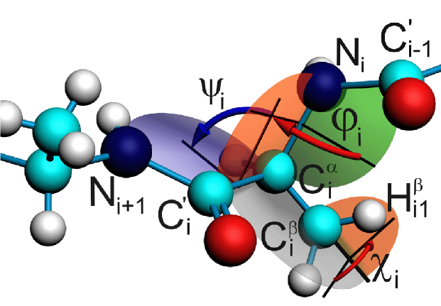
Figure 2: Dihedral angles $\varphi$ and $\psi$ used for characterization of the secondary structure of a polypeptide chain. The dihedral angle $\chi_{i}$ characterizes the rotation of the side radical along the $C_{i}^{\alpha}-C_{i}^{\beta}$ bond.

Both angles are defined by four neighboring atoms in the polypeptide chain. The angle $\varphi_{i}$ is defined as the dihedral angle between the planes formed by the atoms ($C_{i-1}^{{}^{\prime}}-N_{i}-C_{i}^{\alpha}$) and ($N_{i}-C_{i}^{\alpha}-C_{i}^{{}^{\prime}}$). The angle $\psi_{i}$ is defined as the dihedral angle between the ($N_{i}-C_{i}^{\alpha}-C_{i}^{{}^{\prime}}$) and ($C_{i}^{\alpha}-C_{i}^{{}^{\prime}}-N_{i+1}$) planes. The atoms are numbered from the NH₂- terminal of the polypeptide. The angles $\varphi_{i}$ and $\psi_{i}$ take all possible values within the interval [$-180^{\circ}$;$180^{\circ}$]. For the unambiguous definition the angles $\varphi_{i}$ and $\psi_{i}$ are counted clockwise, if one looks on the molecule from its NH₂- terminal (see Fig. 2). This way of angle counting is the most commonly used Rubin (2004); Yakubovich et al. (2006b, c); Solov’yov et al. (2006a, b).

A Hamiltonian function of a polypeptide chain is constructed as a sum of the potential, kinetic and vibrational energy terms. For a polypeptide chain in a particular conformational state $j$ consisting of $n$ amino acids and $N$ atoms we obtain:

$$H_{j}=\frac{{\bf P^{2}}}{2M}+\frac{1}{2}\left(I_{1}^{(j)}\Omega_{1}^{2}+I_{2}^{(j)}\Omega_{2}^{2}+I_{3}^{(j)}\Omega_{3}^{2}\right)+\sum_{i=1}^{3N-6}\frac{p_{i}^{2}}{2m_{i}}+U(\{x\}),$$ (2)

where ${\bf P}$, $M$, $I_{1,2,3}^{(j)}$, $\Omega_{1,2,3}$, are the momentum of the whole polypeptide, its mass, its three main momenta of inertia, and its rotational frequencies. $p_{i}$, $x_{i}$ and $m_{i}$ are the momentum, the coordinate and the generalized mass describing the motion of the system along the $i$-th degree of freedom. $U(\{x\})$ is the potential energy of the system, being the function of all atomic coordinates in the system.

One can group all degrees of freedom in a polypeptide in the two classes: ”stiff” and ”soft” degrees of freedom. We call the degrees of freedom corresponding to the variation of bond lengths, angles and improper dihedral angles (see Fig. 2) as ”stiff”, while degrees of freedom corresponding to the angles $\varphi_{i}$ and $\psi_{i}$ are classified as ”soft” degrees of freedom. The ”stiff” degrees of freedom can be treated within the harmonic approximation because the energies needed for a noticeable change of the system structure with respect to these degrees of freedom are about several eV which is significantly larger than the characteristic thermal energy of the system at room temperature being on the order of $0.026$ eV Solov’yov et al. (2006c, a, b); Scott and van Gunsteren (1995); Cornell et al. (1995); MacKerell. et al. (1998).

The Hamiltonian of the polypeptide can be rewritten in terms of the ”soft” and ”stiff” degrees of freedom. Transforming the set of cartesian coordinates $\{x\}$ to a set of generalized coordinates $\{q\}$, corresponding to the ”soft” and ”stiff” degrees of freedom one obtains:

$$H_{j}=\frac{{\bf P^{2}}}{2M}+\frac{1}{2}\left(I_{1}^{(j)}\Omega_{1}^{2}+I_{2}^{(j)}\Omega_{2}^{2}+I_{3}^{(j)}\Omega_{3}^{2}\right)+\sum_{i=1}^{l_{s}}\sum_{j=l}^{l_{s}}g_{ij}\frac{p_{i}^{s}p_{j}^{s}}{2}$$

$$+\sum_{i=1}^{l_{s}}\sum_{j=l_{s}+1}^{l_{h}}g_{ij}p_{i}^{s}p_{j}^{h}+\sum_{i=l_{s}+1}^{l_{h}}\sum_{j=l_{s}+1}^{l_{h}}g_{ij}\frac{p_{i}^{h}p_{j}^{h}}{2}+U(\{q^{s}\},\{q^{h}\}),$$ (3)

where $q^{s}$ and $q^{h}$ are the generalized coordinates corresponding to the ”soft” and ”stiff” degrees of freedom, and $p^{s}$ and $p^{h}$ are the corresponding generalized momenta. $l_{s}$ and $l_{h}$ is the number of the ”soft” and ”stiff” degrees of freedom in the system, satisfying the relation $3N-6=l_{s}+l_{h}$. $U(\{q^{s}\},\{q^{h}\})$ in Eq. (3) is the potential energy of the system as a function of the ”soft” and ”stiff” degrees of freedom. $1/g_{ij}$ has a meaning of the generalized mass, while $g_{ij}$ is defined as follows:

$$g_{ij}=\sum_{\lambda=1}^{3N-6}\frac{1}{m_{\lambda}}\frac{\partial q_{i}}{\partial x_{\lambda}}\frac{\partial q_{j}}{\partial x_{\lambda}}.$$ (4)

Here $x_{\lambda}$ and $m_{\lambda}$ are the generalized coordinate in the cartesian space and the generalized mass of the system, corresponding to the degree of freedom with index $\lambda$. $q_{i}$ and $q_{j}$ denote the ”soft” or the ”stiff” generalized coordinate in the transformed space.

The motion of the system with respect to its ”soft” and ”hard” degrees of freedom occurs on the different time scales as was discussed in Go and Scheraga (1969). The typical oscillation frequency corresponding to the ”soft” degrees of freedom is on the order of 100 cm^-1, while for the ”stiff” degrees of freedom it is more than 1000 cm^-1 Go and Scheraga (1969). Thus the motion of the system with respect to the ”soft” degrees of freedom is uncoupled from the motion of the system with respect to the ”stiff” degrees of freedom. Therefore the fifth term in Eq. (3), which describes the kinetic energy of the ”stiff” motions in the polypeptide can be diagonalized. The corresponding set of coordinates $\{\tilde{q}^{s}\}$ describes the normal vibration modes in the ”stiff” subsystem:

$$H_{j}=\frac{{\bf P^{2}}}{2M}+\frac{1}{2}\left(I_{1}^{(j)}\Omega_{1}^{2}+I_{2}^{(j)}\Omega_{2}^{2}+I_{3}^{(j)}\Omega_{3}^{2}\right)+\sum_{i=1}^{l_{h}}\left(\frac{\left(\tilde{p}^{h}_{i}\right)^{2}}{2\mu_{i}^{h}}+\frac{\mu_{i}^{h}\omega_{i}^{2}\left(\tilde{q}^{h}_{i}\right)^{2}}{2}\right)$$

$$+\sum_{i=1}^{l_{s}}\sum_{j=1}^{l_{s}}g_{ij}\frac{p_{i}^{s}p_{j}^{s}}{2}+U(\{\chi\})+U(\{\varphi,\psi\}).$$ (5)

Here $\omega_{i}$ and $\mu_{i}^{h}$ are the frequency of the $i$-th ”stiff” normal vibrational mode and the corresponding generalized mass. Note, that the fourth term in Eq. (3) vanishes if the ”soft” and the ”stiff” degrees of freedom are uncoupled. The last two terms in Eq. (5) describe the potential energy of the system in respect to the ”soft” degrees of freedom. For every amino acid there are at least two ”soft” degrees of freedom, corresponding to the angles $\varphi_{i}$ and $\psi_{i}$ (see Fig. 2). Some additional ”soft” degrees of freedom involve the rotation of the side radicals in amino acids. A typical example is the angle $\chi_{i}$, which describes the twisting of the side chain radical along the $C^{\alpha}_{i}-C^{\beta}_{i}$ bond (see Fig. 2). The angle $\chi_{i}$ is defined as the dihedral angle between the planes formed by the atoms ($C_{i}^{{}^{\prime}}-C_{i}^{\alpha}-C_{i}^{\beta}$) and by the bonds $C_{i}^{\alpha}-C_{i}^{\beta}$ and $C_{i}^{\beta}-H_{i1}^{\beta}$. Note, that the notations $\chi$, $\varphi$ and $\psi$ are used for the simplicity and for the further explanation of our theory. The set of these dihedral angles builds up the set of ”soft” degrees of freedom of the polypeptide: $\{q^{s}\}\equiv\{\chi,\varphi,\psi\}$.

Note that generalized masses $1/g_{ij}$ depend on the choice of the generalized coordinates in the system. However this dependence can be neglected if the system is considered in the vicinity of its equilibrium state. In this case the motion of the polypeptide with respect to the ”soft” degrees of freedom can be considered as the motion of the system of coupled nonlinear oscillators. In the vicinity of the system’s equilibrium state the generalized mass can be written as:

$$\frac{1}{g_{ij}}=\frac{1}{g_{ij}\left(\{q^{s}_{i_{0}}\}\right)}+\sum_{k=1}^{l_{s}}\left.\frac{\partial\left(1/g_{ij}\right)}{\partial q^{s}_{k}}\right|_{q_{k}^{s}=q_{k_{0}}^{s}}\left(q_{k}^{s}-q_{k_{0}}^{s}\right),$$ (6)

where $q_{k_{0}}^{s}$ denotes the value of the $k$-th ”soft” degree of freedom at the equilibrium position. The second term in Eq. (6) describes the dependence of the generalized mass on coordinates and can be neglected if the system is in the vicinity of its equilibrium. All the information about the nonlinearity of the oscillations is contained in the potential energy functions $U(\{\chi\})$ and $U(\{\varphi,\psi\})$ in Eq. (5).

The validity of the coordinate-independent mass approximation was also discussed in Ref. Go and Scheraga (1969). In the present paper we do not account for the coordinate dependence of the generalized masses, $g_{ij}$, and leave this question open for further investigation.

II.2 Partition function

The partition function of the polypeptide is constructed within the framework of classical mechanics. We consider the classical partition function because in our following paper Yakubovich et al. (2007b) we have treated the polypeptide classically. However the presented formalism can be easily generalized for the quantum mechanical description of the system.

All thermodynamic properties of a system are determined by its partition function, which can be expressed via the system’s Hamiltonian in the following form Landau and Lifshitz (1959):

$${\mathbb{Z}}=\int\exp\left(-\frac{H}{kT}\right)d\Gamma,$$ (7)

where $H$ is the Hamiltonian of the system, $k$ and $T$ are the Boltzmann constant and the temperature respectively and $d\Gamma$ is an element of the phase space. Substituting (5) into (7) one obtains an expression for the partition function of a polypeptide in a particular conformational state $j$. Thus, the partition function of the system can be factored as follows:

$${\mathbb{Z}}=\frac{1}{\left(2\pi\hbar\right)^{3N}}Z_{1}\cdot Z_{2}\cdot Z_{3}\cdot Z_{4}\cdot Z_{5},$$ (8)

where

$$Z_{1} = \int\exp\left(\frac{1}{kT}\left[-\frac{{\bf P^{2}}}{2M}-\left(\frac{{\cal M}_{1}^{2}}{2I_{1}^{(j)}}+\frac{{\cal M}_{2}^{2}}{2I_{2}^{(j)}}+\frac{{\cal M}_{3}^{2}}{2I_{3}^{(j)}}\right)\right]\right){\rm d^{3}}P\cdot{\rm d^{3}}Q\cdot{\rm d^{3}}{\cal M}\cdot{\rm d^{3}}\Phi=$$ (9)

$$=64\pi^{5}V_{j}M^{3/2}\sqrt{I_{j}^{(1)}I_{j}^{(2)}I_{j}^{(3)}}(kT)^{3}$$

$$Z_{2} = \int\exp\left(-\frac{1}{kT}\sum_{i=1}^{l_{h}}\left(\frac{\left(\tilde{p}^{h}_{i}\right)^{2}}{2\mu_{i}^{h}}+\frac{\mu_{i}^{h}\omega_{i}^{2}\left(\tilde{q}^{h}_{i}\right)^{2}}{2}\right)\right){\rm d^{l_{h}}}\tilde{p}^{h}\cdot{\rm d^{l_{h}}}\tilde{q}^{h}=\frac{\left(2\pi kT\right)^{l_{h}}}{\prod_{i=1}^{l_{h}}\omega_{i}},$$ (10)

$$Z_{3} = \int\exp\left(-\frac{1}{kT}\sum_{i=1}^{l_{s}}\frac{\left(\tilde{p}^{s}_{i}\right)^{2}}{2\mu_{i}^{s}}\right){\rm d^{l_{s}}}\tilde{p}^{s}=\sqrt{\left(2\pi kT\right)}^{l_{s}}\prod_{i=1}^{l_{s}}\sqrt{\mu_{i}^{s}},$$ (11)

$$Z_{4} = \int\exp\left(-\frac{U(\{\tilde{\chi}\})}{kT}\right){\rm d^{l_{\chi}}}\tilde{\chi}^{s},$$ (12)

$$Z_{5} = \frac{1}{\left(2\pi\hbar\right)^{(l_{\varphi}+l_{\psi})/2}}\int\exp\left(-\frac{U(\{\tilde{\varphi},\tilde{\psi}\})}{kT}\right){\rm d^{l_{\varphi}}}\tilde{\varphi}^{s}\cdot{\rm d^{l_{\psi}}}\tilde{\psi}^{s}.$$ (13)

$Z_{1}$, Eq. (9), describes the contribution to the partition function originating from the motion of the polypeptide as a rigid body. Here $V_{j}$ is the specific volume of the polypeptide in conformational state $j$ and ${\cal M}$ is the angular momenta of the polypeptide. $Z_{2}$, Eq. (10), accounts for the ”stiff” degrees of freedom in the polypeptide. $Z_{3}$, Eq. (11), describes the contribution of the kinetic energy of the ”soft” degrees of freedom to the partition function. $Z_{4}$, Eq. (12), and $Z_{5}$, Eq. (13), describe the contribution of the potential energy of the ”soft” degrees of freedom to the partition function. Integrating over the phase space in Eqs. (9)-(13) is performed over generalized coordinates and momentum space.

For the derivation of Eqs. (11)-(13) we have diagonalized the quadratic form of the generalized momenta corresponding to the ”soft” degrees of freedom in Eq. (5) and made a transformation $q_{i}^{s}\rightarrow{\tilde{q}}_{i}^{s}$, $p_{i}^{s}\rightarrow{\tilde{p}}_{i}^{s}$. In Eq. (11), $\mu_{i}^{s}$ is the generalized mass of the $i$-th ”soft” normal vibration mode, being related to $g_{ij}$ in Eq. (4). ${\tilde{\chi}}$,${\tilde{\varphi}}$ and ${\tilde{\psi}}$ in Eqs. (12)-(13) denote the ”soft” twisting degrees of freedom, which have been transformed accordingly. Note that $\tilde{q}_{i}^{s}$ and $\tilde{p}_{i}^{s}$ are canonical conjugated coordinates. $l_{\chi}$, $l_{\varphi}$ and $l_{\psi}$ in Eqs. (12)-(13) is the number of the $\chi$, $\varphi$ and $\psi$ degrees of freedom in the system. Note, that $l_{s}=l_{\chi}+l_{\varphi}+l_{\psi}$.

Integrals in Eqs. (9)-(11) can be evaluated analytically, while for the integration over the angles $\chi$, $\varphi$ and $\psi$ in Eqs. (12)-(13) the knowledge of the exact potential energy surface of the polypeptide is necessary. However the potential energy of the polypeptide corresponding to the twisting degrees of freedom $\chi$ does not depend on the conformation of the polypeptide in case of neutral non-polar radicals in simple amino acids (i.e. alanine, glycine) Go and Scheraga (1969). Thus, the twisting degrees of freedom corresponding to the variations of angles $\chi$ have a minor influence on the $\alpha$-helix$\leftrightarrow$random coil phase transition. The potential energy of the polypeptide in respect to these degrees of freedom is well described by the following function, as follows from the molecular mechanics potential Eq. (1):

$$U(\chi_{i})=k_{\chi_{i}}\left[1+\cos\left(3\chi_{i}\right)\right],$$ (14)

where $k_{\chi_{i}}$ is the stiffness parameter of the potential. Since $k_{\chi_{i}}=k_{\chi}$, substituting Eq. (14) into Eq. (12) and integrating over $2\pi$ one obtains:

$$Z_{4} = \left[2\pi\exp\left(-\frac{k_{\chi}}{kT}\right){\rm I_{0}}\left(\frac{k_{\chi}}{kT}\right)\right]^{l_{\chi}}=(2\pi)^{l_{\chi}}B(kT),$$ (15)

where ${\rm I_{0}}(x)$ is the the modified Bessel function of the first kind, and $B(kT)=\left[\exp\left(-\frac{k_{\chi}}{kT}\right){\rm I_{0}}\left(\frac{k_{\chi}}{kT}\right)\right]^{l_{\chi}}$.

Substituting $Z_{1}$-$Z_{5}$ into Eq. (8) one obtains the expression for the partition function of a polypeptide in a particular conformational state $j$:

$$Z_{j} = \left[\frac{V_{j}\cdot M^{3/2}\cdot\sqrt{I_{j}^{(1)}I_{j}^{(2)}I_{j}^{(3)}}\prod_{i=1}^{l_{s}}\sqrt{\mu_{i}^{s}}}{(2\pi)^{\frac{l_{s}}{2}-l_{\chi}}\pi\hbar^{3N}\prod_{i=1}^{l_{h}}\omega_{i}}\right]B(kT)\cdot(kT)^{3N-3-\frac{l_{s}}{2}}$$ (16)

$$\int_{-\pi}^{\pi}\ldots\int_{-\pi}^{\pi}e^{-\frac{U(\{\varphi,\psi\})}{kT}}{\rm d}\varphi_{1}\ldots{\rm d}\varphi_{n}\ {\rm d}\psi_{1}\ldots{\rm d}\psi_{n}=$$

$$= A_{j}\cdot B(kT)\cdot(kT)^{3N-3-\frac{l_{s}}{2}}\int_{-\pi}^{\pi}\ldots\int_{-\pi}^{\pi}e^{-\frac{U(\{\varphi,\psi\})}{kT}}{\rm d}\varphi_{1}\ldots{\rm d}\varphi_{n}\ {\rm d}\psi_{1}\ldots{\rm d}\psi_{n},$$

$A_{j}$ denotes the factor in the square brackets. Note, that generalized masses $\mu_{i}^{h}$ are reduced during the integration and do not enter into the expression of the partition function.

Since a polypeptide exist in different conformational states, one needs to sum over the contributions of all possible conformations $Z_{j}$ in order to calculate the complete partition function of the polypeptide. For an ensemble of ${\cal N}$ noninteracting polypeptides the partition function reads as

$${\mathbb{Z}}=\left(\sum_{j=1}^{\xi}Z_{j}\right)^{\cal N} = \left(B(kT)\cdot(kT)^{3N-3-\frac{l_{s}}{2}}\sum_{j=1}^{\xi}A_{j}\right.$$ (17)

$$\left.\cdot\int_{-\pi}^{\pi}\ldots\int_{-\pi}^{\pi}e^{-\frac{U(\{\varphi,\psi\})}{kT}}{\rm d}\varphi_{1}\ldots{\rm d}\varphi_{n}\ {\rm d}\psi_{1}\ldots{\rm d}\psi_{n}\right)^{\cal N},$$

where $Z_{j}$ is defined in (16) and $\xi$ is the total number of possible conformations in a polypeptide. Equation (17) has been derived with a minimum number of assumptions about the system. It is general, however, its use for a particular molecular systems is not so straightforward. Expression (17) can be further simplified, if one makes additional assumptions about the structure of the system.

For the sake of simplicity, we write further equations for only one polypeptide instead of ${\cal N}$. Generalization for the case of ${\cal N}$ statistically independent polypeptides can always be done according to (17).

One can expect that the factors $A_{j}$ in (17) depend on the chosen conformation of the polypeptide. However, due to the fact that the values of specific volumes, momenta of inertia and frequencies of normal vibration modes of the polypeptide in different conformations are expected to be close Krimm and Bandekar (1980); Yakubovich et al. (2006a), the values of $A_{j}$ in all these conformations can be considered as equal, at least in the zero order approximation. Thus $A_{j}\equiv A$.

The amino acids can be treated as statistically independent in any conformation of the polypeptide. This fact is not obvious and it was not systematically investigated so far. The statistical independence of small neutral non-polar amino acids (alanine, glycine, etc) in a polypeptide was studied in Rubin (2004) with the use of time-correlation functions between different amino acids. In our following paper Yakubovich et al. (2007b), we address this question for alanine polypeptides and determine the degree to which amino acids in the polypeptide can be treated as statistically independent.

With the assumptions made, the partition function of polypeptide reduces to:

$${\mathbb{Z}}=A\cdot B(kT)\cdot(kT)^{3N-3-\frac{l_{s}}{2}}\sum_{j=1}^{\xi}\prod_{i=1}^{n}\int_{-\pi}^{\pi}\int_{-\pi}^{\pi}\exp\left({-\frac{\epsilon_{i}^{(j)}(\varphi,\psi)}{kT}}\right){\rm d}\varphi{\rm d}\psi,$$ (18)

where $\epsilon_{i}^{(j)}(\varphi,\psi)$ is the potential energy of $i$-th amino acid in the polypeptide, being in one of its $\xi$ conformations denoted with $j$. The potential energy of the amino acid is calculated as a function of its twisting degrees of freedom $\varphi$ and $\psi$.

In equation (18) the partition function is summed over all conformations of the polypeptide. However, in the case of the $\alpha$-helix to random coil transition of the polypeptide, the summation over the polypeptide conformations has to be performed only over the conformations involved in the transition.

Note that Eq. (18) is rather general and can be used for the description of the folding process in proteins. Indeed, the partition function in Eq. (18) is determined by the potential energy surfaces of amino acid in the native state of a protein and in the random coil conformation. The potential energy surfaces can be calculated on the basis of ab initio DFT, combined with molecular mechanics theories as demonstrated in Yakubovich et al. (2006a, 2007a) and in the following paper Yakubovich et al. (2007b). For a protein, which has 20 different amino acids it is necessary to calculate at least 40 different potential energy surfaces, while for the study of folding of polypeptide consisting of the identical amino acids a single potential energy surface describes the transition.

Further simplifications of the partition function (18) for polypeptide consisting of the identical amino acids can be achieved if one assumes that each amino acid in the polypeptide can occupy two states only, below referred as the bounded and unbounded states. The amino acid is considered to be in the bounded state when it forms one hydrogen bond with the neighboring amino acids. In the unbounded state amino acids do not have hydrogen bonds. When the $\alpha$-helix is formed, all amino acids are in the bounded state, while in the case of random coil all amino acids occupy the unbounded states.

All possible conformations of the polypeptide experiencing in the course of the $\alpha$-helix$\leftrightarrow$random coil phase transition can be divided in three different groups:

• completely folded state of the polypeptide ($\alpha$-helix), in which all the amino acids occupy bounded states.

• partially folded states of the polypeptide (phase co-existence), in which the core of $\lambda$ amino acids of the polypeptide occupy bounded states, and $n-\lambda$ boundary amino acids are in unbounded states.

• completely unfolded state of a polypeptide (random coil), in which all the amino acids are in unbounded states.

• phase mixing, in which two or more fragments of a polypeptide are in an $\alpha$-helix state, while the amino acids between the fragments are in the random coil state.

With the assumptions outlined above and assuming the polypeptide to consist of $n$ identical amino acids the partition function (18) of the system can be rewritten as follows:

$${\mathbb{Z}} = A\cdot B(kT)\cdot(kT)^{3N-3-\frac{l_{s}}{2}}\left[\beta Z_{b}^{n-1}Z_{u}+\beta\sum_{i=1}^{n-4}(i+1)Z_{b}^{n-i-1}Z_{u}^{i+1}+Z_{u}^{n}+\right.$$ (19)

$$\left.+\sum_{i=2}^{(n-3)/2}\beta^{i}\sum_{k=i}^{n-i-3}\frac{(k-1)!(n-k-3)!}{i!(i-1)!(k-i)!(n-k-i-3)!}Z_{b}^{k+3i}Z_{u}^{n-k-3i}\right]$$

Here the first and the third terms in the square brackets describe the partition function of the polypeptide in the $\alpha$-helix and in the random coil phases respectively, while the second term in the square brackets accounts for situation of the phase co-existence. The summation in the second term in (19) is performed up to $n-4$, because the shortest $\alpha$-helix consists of 4 amino acids. The last term in the square brackets accounts for the polypeptide conformations in which a number of amino acids being in the helix conformation are separated by amino acids being in the random coil conformation. The first summation in this term goes over the separated helical fragments of the polypeptide, while the second summation goes over individual amino acids in the corresponding fragment. Polypeptide conformations with two or more helical fragments are energetically unfavorable. This fact is discussed in our following paper Yakubovich et al. (2007b). As shown in the following paper Yakubovich et al. (2007b) the contribution to the partition function represented by the fourth term in the square brackets in Eq. (19) is significantly small when compared to the first three terms, for polypeptides containing less than 100 of amino acids. Therefore, it can be omitted in the construction of the partition function. $Z_{b}$ and $Z_{u}$ are the contributions to the partition function from a single amino acid being in the bounded or unbounded states respectively, they read as:

$$Z_{b} = \int_{-\pi}^{\pi}\int_{-\pi}^{\pi}\exp\left({-\frac{\epsilon^{(b)}(\varphi,\psi)}{kT}}\right){\rm d}\varphi{\rm d}\psi$$ (20)

$$Z_{u} = \int_{-\pi}^{\pi}\int_{-\pi}^{\pi}\exp\left({-\frac{\epsilon^{(u)}(\varphi,\psi)}{kT}}\right){\rm d}\varphi{\rm d}\psi$$ (21)

$$\beta = \left(\int_{-\pi}^{\pi}\int_{-\pi}^{\pi}\exp\left({-\frac{\epsilon^{(b)}(\varphi,\psi)+\epsilon^{(u)}(\varphi,\psi)}{kT}}\right){\rm d}\varphi{\rm d}\psi\right)^{3},$$ (22)

where $\epsilon^{(b)}(\varphi,\psi)$ and $\epsilon^{(u)}(\varphi,\psi)$ are the potential energies of a single amino acid being in the bounded or in the unbounded states respectively calculated versus the twisting degrees of freedom $\varphi$ and $\psi$. $\beta$ is a factor accounting for the entropy loss of the helix initiation. Substituting (20), (21) and (22) into equation (19) one obtains the final expression for the partition function of polypeptide undergoing an $\alpha$-helix$\leftrightarrow$random coil phase transition. This result can be used for the evaluation of all thermodynamical characteristics of the system.

$\epsilon^{(b)}(\varphi,\psi)$ and $\epsilon^{(u)}(\varphi,\psi)$ determine the partition function of polypeptide. These quantities can be calculated on the basis of ab initio DFT, combined with molecular mechanics theories as demonstrated in Yakubovich et al. (2006a, 2007a) and in the following paper Yakubovich et al. (2007b).

III Thermodynamical characteristics of a polypeptide chain

The first order phase transition is characterized by an abrupt change of the internal energy of the system with respect to its temperature. In the first order phase transition the system either absorbs or releases a fixed amount of energy while heat capacity as a function of temperature has a sharp peak Finkelstein and Ptitsyn (2002); Landau and Lifshitz (1959) (see Fig. 3).

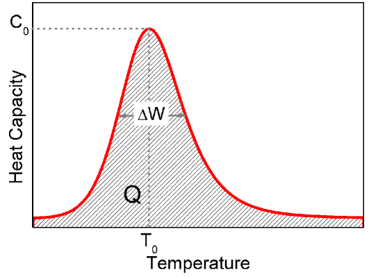
Figure 3: Temperature dependence of the heat capacity for a system experiencing a phase transition.

The peak in the heat capacity is characterized by the transition temperature $T_{0}$, the maximal value of the heat capacity $C_{0}$, the temperature range of the phase transition $\Delta W$ and the specific heat $Q$, which is also referred as the latent heat of the phase transition (see Fig. 3).

All these quantities can be calculated if the dependence of the heat capacity on temperature is known. The temperature dependence of the heat capacity is defined by the partition function as follows Landau and Lifshitz (1959):

$$C(T)=kT\frac{\partial^{2}T\ln{\mathbb{Z}}}{\partial T^{2}}.$$ (23)

The characteristics of the phase transition are determined by the following equations:

$$\left.\frac{dC(T)}{dT}\right|_{T=T_{0}}=0$$ (24)

$$C_{0}=C(T_{0})$$ (25)

$$C(T_{0}\pm\Delta W)=\frac{C_{0}}{2}$$ (26)

$$Q=\int_{0}^{\infty}C(T){\rm d}T.$$ (27)

Unfortunately it is not possible to obtain analytical expressions for $T_{0}$, $C_{0}$, $\Delta W$ and $Q$ with partition function defined in (19) because the integrals in (20) and (21) can not be treated analytically. However, the qualitative behavior of these quantities can be understood if one assumes that all conformational states of a polypeptide in a certain phase have the same energy. This model is usually referred to in literature as the two-energy-level model Prabhu and Sharp (2005); Yakubovich et al. (2006a, 2007a) and it turns out to be very useful for the qualitative analysis of the phase transitions in polypeptide chains. If one considers the phase transition between two such phases, the partition function can then be constructed as follows:

$${\mathbb{Z}}\approx{\mathbb{Z}_{0}}\left[1+A\frac{\eta_{2}}{\eta_{1}}e^{-\frac{\Delta E}{kT}}\right],$$ (28)

where ${\mathbb{Z}_{0}}$ is the partition function of the system in the first phase, $\Delta E=E_{2}-E_{1}$ is the energy difference between the states of the polypeptide in two different phases, $\eta_{1}$ and $\eta_{2}$ are the numbers of isomeric states of the polypeptide in the first and in the second phases respectively. They can also be considered as the population of the two phases. $A=A_{2}/A_{1}$ is the coefficient depending on masses, specific volumes, normal vibration modes frequencies and momenta of inertia of the polypeptide in the two phases. Substituting equation (28) into equation (23) one obtains the expression for the heat capacity in the framework of the two-energy-level model:

$$C(T)=\frac{A\frac{\eta_{2}}{\eta_{1}}\Delta E^{2}e^{-\left(\frac{\Delta E}{kT}\right)}}{kT^{2}\left(1+A\frac{\eta_{2}}{\eta_{1}}e^{-\left(\frac{\Delta E}{kT}\right)}\right)^{2}}.$$ (29)

Substituting equation (29) into equations (24)-(27) and solving them one obtains the expressions for $T_{0}$, $C_{0}$, $\Delta W$ and $Q$, which read as:

$$T_{0} \approx \frac{{\Delta E}}{k\ln\left(A\frac{\eta_{2}}{\eta_{1}}\right)}=\frac{{\Delta E}}{\Delta S},$$ (30)

$$C_{0} \approx \frac{k}{4}\left[\ln\left(A\frac{\eta_{2}}{\eta_{1}}\right)\right]^{2}=\frac{\Delta S^{2}}{4k},$$ (31)

$$\Delta W \approx \sqrt{\frac{64\ln 2}{\pi}}\frac{\Delta E}{k\left[\ln\left(A\frac{\eta_{2}}{\eta_{1}}\right)\right]^{2}}=\sqrt{\frac{64\ln 2}{\pi}}\frac{k\Delta E}{\Delta S^{2}},$$ (32)

$$Q = \int C(T){\rm d}T=\Delta E.$$ (33)

Here $\Delta S=k\ln{A\eta_{2}}-k\ln{\eta_{1}}$ is the entropy change in the system and $M$ is the mass of a single polypeptide. $\Delta S$ and $\Delta E$ are the major thermodynamical parameters in the considered problem, since they determine the behavior of the phase transition characteristics. From equations (30)-(32) follows, that $T_{0}\sim\frac{{\Delta E}}{\Delta S}$, $C_{0}\sim\Delta S^{2}$, $Q\sim\Delta E$ and $\Delta W\sim\frac{\Delta E}{\Delta S^{2}}$.

The numerical calculation and analysis of various thermodynamical characteristics such as the latent heat or the heat capacity is done in the following paper Yakubovich et al. (2007b).

IV Conclusion

In the present paper a novel ab initio theoretical method for treating the $\alpha$-helix$\leftrightarrow$random coil phase transition in polypeptide chains is introduced. The suggested method is based on the construction of a parameter-free partition function for a system undergoing a first order phase transition. All the necessary information for the construction of such a partition function can be calculated on the basis of ab initio DFT, combined with molecular mechanics theories (see results of numerical simulations in the following paper Yakubovich et al. (2007b)).

The suggested method is considered as an efficient alternative to the existing theoretical approaches for the study of helix-coil transition in polypeptides since it does not contain any model parameters. It gives a universal recipe for statistical mechanics description of complex molecular systems. The partition function of polypeptide is written with a minimum number of assumptions about the system which makes our method much more general and universal in comparison with other theoretical approaches.

In the present paper we introduced novel theoretical method for the study of $\alpha$-helix$\leftrightarrow$random coil phase transition in polypeptides. In the following paper Yakubovich et al. (2007b) we report the results of numerical simulations of this process obtained within the framework of the suggested model.

V Acknowledgments

We acknowledge support of this work by the NoE EXCELL, by INTAS under the grant 03-51-6170. We are grateful to Ms. Stephanie Lo for critical reading of the manuscript and several suggestions for improvement.

References

- Shakhnovich (2006) E. Shakhnovich, Chem. Rev. 106, 1559 (2006).
- Finkelstein and Ptitsyn (2002) A. Finkelstein and O. Ptitsyn, Protein Physics. A Course of Lectures (Elsevier Books, Oxford, 2002).
- Shea and Brooks (2001) J.-E. Shea and C. L. Brooks, Ann. Rev. Phys. Chem. 52, 499 (2001).
- Prabhu and Sharp (2005) N. V. Prabhu and K. A. Sharp, Ann. Rev. Phys. Chem. 56, 521 (2005).
- Yakubovich et al. (2007a) A. Yakubovich, I. Solov’yov, A. Solov’yov, and W. Greiner, Europhys. News 38, 10 (2007a).
- Yakubovich et al. (2006a) A. Yakubovich, I. Solov’yov, A. Solov’yov, and W. Greiner, Eur. Phys. J. D 40, 363 (2006a).
- Zimm and Bragg (1959) B. Zimm and J. Bragg, J. Chem. Phys. 31, 526 (1959).
- Gibbs and DiMarzio (1959) J. Gibbs and E. DiMarzio, J. Phys. Chem. 30, 271 (1959).
- Lifson and Roig (1961) S. Lifson and A. Roig, J. Chem. Phys. 34, 1963 (1961).
- Schellman (1958) J. A. Schellman, J. Phys. Chem. 62, 1485 (1958).
- Lifson (1964) S. Lifson, J. Chem. Phys. 40, 3705 (1964).
- Poland and Scheraga (1966a) D. Poland and H. A. Scheraga, J. Chem. Phys. 45, 1456 (1966a).
- Poland and Scheraga (1966b) D. Poland and H. A. Scheraga, J. Chem. Phys. 45, 2071 (1966b).
- Go and Scheraga (1976) N. Go and H. A. Scheraga, Macromolecules 9, 535 (1976).
- Go and Scheraga (1969) N. Go and H. A. Scheraga, J. Chem. Phys. 51, 4751 (1969).
- Ooi and Oobatake (1991) T. Ooi and M. Oobatake, Proc. Natl. Acad. Sci. USA 88, 2859 (1991).
- Gomez et al. (1995) J. Gomez, V. J. Hilser, D. Xie, and E. Freire, Proteins: Struct., Func., Gen. 22, 404 (1995).
- Tobias and Brooks (1991) D. J. Tobias and C. L. Brooks, Biochemistry 30, 6059 (1991).
- Garcia and Sanbonmatsu (2002) A. E. Garcia and K. Y. Sanbonmatsu, Proc. Natl. Acad. Sci. USA 99, 2781 (2002).
- Nymeyer and Garcia (2003) H. Nymeyer and A. E. Garcia, Proc. Natl. Acad. Sci. USA 100, 13934 (2003).
- Irbäck and Sjunnesson (2004) A. Irbäck and F. Sjunnesson, Proteins: Struct., Func., Gen. 56, 110 (2004).
- Shental-Bechor et al. (2005) D. Shental-Bechor, S. Kirca, N. Ben-Tal, and T. Haliloglu, Biophys. J. 88, 2391 (2005).
- Scott and van Gunsteren (1995) W. Scott and W. van Gunsteren, in Methods and Techniques in Computational Chemistry: METECC-95, edited by E. Clementi and G. Corongiu (STEF, Cagliari, Italy, 1995), pp. 397–434.
- Cornell et al. (1995) W. Cornell, P. Cieplak, C. Bayly, I. Gould, K. M. Jr., D. Ferguson, D. Spellmeyer, T. Fox, J. Caldwell, and P. Kollman, J. Am. Chem. Soc. 117, 5179 (1995).
- MacKerell. et al. (1998) A. MacKerell., D. Bashford, R. Bellott, R. Dunbrack, J. Evanseck, M. Field, S. Fischer, J. Gao, H. Guo, S. Ha, et al., J. Phys. Chem. B 102, 3586 (1998).
- Chen et al. (2005) C. Chen, Y. Xiao, and L. Zhang, Biophys. J. 88, 3276 (2005).
- Duan and Kollman (1998) Y. Duan and P. A. Kollman, Science 282, 740 (1998).
- Liwo et al. (2005) A. Liwo, M. Khalili, and H. A. Scheraga, Proc. Natl. Acad. Sci. USA 102, 2362 (2005).
- Ding et al. (2002) F. Ding, N. V. Dokholyan, S. V. Buldyrev, H. E. Stanley, and E. I. Shakhnovich, Biophys. J. 83, 3525 (2002).
- Pande et al. (2002) V. S. Pande, I. Baker, J. Chapman, S. P. Elmer, S. M. Larson, Y. M. Rhee, M. R. Shirts, C. D. Snow, E. J. Sorin, and B. Zagrovic, Biopolymers 68, 91 (2002).
- Irbäck et al. (2003) A. Irbäck, B. Samuelsson, F. Sjunnesson, and S. Wallin, Biophys. J. 85, 1466 (2003).
- Kubelka et al. (2004) J. Kubelka, J. Hofrichter, and W. A. Eaton, Curr. Opin. Struct. Biol. 14, 76 (2004).
- Lipman et al. (2003) E. A. Lipman, B. Schuler, O. Bakajin, and W. A. Eaton, Science 301, 1233 (2003).
- He and Scheraga (1998a) S. He and H. A. Scheraga, J. Chem. Phys. 108, 271 (1998a).
- He and Scheraga (1998b) S. He and H. A. Scheraga, J. Chem. Phys. 108, 287 (1998b).
- Fujita et al. (1981) S. Fujita, E. Blaisten-Borojas, M. Torres, and S. V. Godoy, J. Chem. Phys. 75, 3097 (1981).
- Cárdenas and Elber (2003) A. E. Cárdenas and R. Elber, Biophys. J. 85, 2919 (2003).
- Scholtz et al. (1991) J. M. Scholtz, S. Marqusee, R. L. Baldwin, E. J. York, J. M. Stewart, M. Santoro, and D. W. Bolen, Proc. Natl. Acad. Sci. USA 88, 2854 (1991).
- Lednev et al. (2001) I. K. Lednev, A. S. Karnoup, M. C. Sparrow, and S. A. Asher, J. Am. Chem. Soc. 123, 2388 (2001).
- Thompson et al. (1997) P. A. Thompson, W. A. Eaton, and J. Hofrichter, Biochemistry 36, 9200 (1997).
- Williams et al. (1996) S. Williams, R. G. Thimothy P. Causgrove, K. S. Fang, R. H. Callender, W. H. Woodruff, and R. B. Dyer, Biochemistry 35, 691 (1996).
- Kromhout and Linder (2001) R. A. Kromhout and B. Linder, J. Phys. Chem. B 105, 4987 (2001).
- Chakrabartty et al. (1994) A. Chakrabartty, T. Kortemme, and R. L. Baldwin, Prot. Sci. 3, 843 (1994).
- Go et al. (1970) M. Go, N. Go, and H. A. Scheraga, J. Chem. Phys. 52, 2060 (1970).
- Scheraga et al. (2002) H. A. Scheraga, J. A. Villa, and D. R. Ripoll, Biophys. Chem. 01-102, 255 (2002).
- Wójcik et al. (1990) J. Wójcik, K.-H. Altmann, and H. Scheraga, Biopolymers 30, 121 (1990).
- Scott and Scheraga (1966) R. A. Scott and H. A. Scheraga, J. Chem. Phys. 45, 2091 (1966).
- Ooi et al. (1967) T. Ooi, R. A. Scott, G. Vanderkooi, and H. A. Scheraga, J. Chem. Phys. 46, 4410 (1967).
- Wang et al. (1995) L. Wang, T. O’Connell, A. Tropsha, and J. Hermans, Proc. Natl. Acad. Sci. USA 92, 10924 (1995).
- Yakubovich et al. (2007b) A. Yakubovich, I. Solov’yov, A.V.Solov’yov, and W.Greiner, Eur. Phys. Journ. D, following paper (2007b).
- Foresman and leen Frisch (1996) J. B. Foresman and A. leen Frisch, Exploring Chemistry with Electronic Structure Methods (Pittsburgh, PA: Gaussian Inc, 1996).
- Yakubovich et al. (2006b) A. Yakubovich, I. Solov’yov, A. Solov’yov, and W. Greiner, Eur. Phys. J. D 39, 23 (2006b).
- Yakubovich et al. (2006c) A. Yakubovich, I. Solov’yov, A.V.Solov’yov, and W.Greiner, Khimicheskaya Fizika (Chemical Physics) (in Russian) 25, 11 (2006c).
- Solov’yov et al. (2006a) I. Solov’yov, A. Yakubovich, A. Solov’yov, and W. Greiner, Phys. Rev. E 73, 021916 (2006a).
- Solov’yov et al. (2006b) I. Solov’yov, A. Yakubovich, A.V.Solov’yov, and W.Greiner, J. Exp. Theor. Phys. 102, 314 (2006b), original Russian Text, published in Zhurnal Eksperimental’noi i Teoreticheskoi Fiziki, 129, p. 356-370 (2006).
- Rubin (2004) A. Rubin, Biophysics: Theoretical Biophysics (Moscow University Press ”Nauka”, 2004).
- Solov’yov et al. (2006c) I. Solov’yov, A. Yakubovich, A. Solov’yov, and W. Greiner, J. Exp. Theor. Phys. 103, 463 (2006c), original Russian Text, published in Zhurnal Eksperimental’noi i Teoreticheskoi Fiziki, 130, 534-543 (2006).
- Landau and Lifshitz (1959) L. Landau and E. Lifshitz, Statistical Physics (London-Paris, Pergamon Press, 1959).
- Krimm and Bandekar (1980) S. Krimm and J. Bandekar, Biopolymers 19, 1 (1980).