Computation in Sofic Quantum Dynamical Systems

Abstract

We analyze how measured quantum dynamical systems store and process information, introducing sofic quantum dynamical systems. Using recently introduced information-theoretic measures for quantum processes, we quantify their information storage and processing in terms of entropy rate and excess entropy, giving closed-form expressions where possible. To illustrate the impact of measurement on information storage in quantum processes, we analyze two spin-$1$ sofic quantum systems that differ only in how they are measured.

I Introduction

Extending concepts from symbolic dynamics to the quantum setting, we forge a link between quantum dynamical systems and quantum computation, in general, and with quantum automata, in particular.

Symbolic dynamics originated as a method to study general dynamical systems when, nearly 100 years ago, Hadamard used infinite sequences of symbols to analyze the structure of geodesics on manifolds of negative curvature; see Ref. [1] and references therein. In the 1930’s and 40’s Hedlund and Morse coined the term symbolic dynamics [2, 3] to describe the study of dynamics over the space of symbol sequences in their own right. In the 1940’s Shannon used sequence spaces to describe information channels [4]. Subsequently, the techniques and ideas have found significant applications beyond dynamical systems, in data storage and transmission, as well as in linear algebra [5].

On the flip side of the same coin, computation theory codes symbol sequences using finite-state automata. The class of sequences that can be coded this way define the regular languages [6]. It turns out that many dynamical systems can also be coded with finite-state automata using the tools of symbolic dynamics [5]. In fact, Sofic systems are the particular class of dynamical systems that are the analogs of regular languages in automata theory.

The study of quantum behavior in classically chaotic systems is yet another active thread in dynamical systems [7, 8] which has most recently come to address the role of measurement. Measurement interaction leads to genuinely chaotic behavior in quantum systems, even far from the semi-classical limit [9]. Classical dynamical systems can be embedded in quantum dynamical systems as the special class of commutative dynamical systems, which allow for unambiguous assignment of joint probabilities to two observations [10].

An attempt to construct symbolic dynamics for quantum dynamical systems was made by Alicki and Fannes [10], who defined shifts on spin chains as the analog of shifts in sequence space. Definitions of entropy followed from this. However, no connection to quantum finite-state automata was established there.

In the following we develop an approach that differs from this and other previous attempts since it explicitly accounts for observed sequences, in contrast to sequences of (unobservable) quantum objects, such as spin chains. The recently introduced computational model class of quantum finite-state generators provides the required link between quantum dynamical systems and the theory of automata and formal languages [11]. It gives access to an analysis of quantum dynamical systems in terms of symbolic dynamics. Here, we strengthen that link by studying explicit examples of quantum dynamical systems. We construct their quantum finite-state generators and establish their sofic nature. In addition we review tools that give an information-theoretic analysis for quantifying the information storage and processing of these systems. It turns out that both the sofic nature and information processing capacity depend on the way a quantum system is measured.

II Quantum finite-state generators

To start, we recall the quantum finite-state generators (QFGs) defined in Ref. [11]. They consist of a finite set of internal states $Q=\{q_{i}:i=1,\ldots,|Q|\}$. The state vector is an element of a $|Q|$-dimensional Hilbert space: $\mathinner{\langle{\psi}|}\in\mathcal{H}$. At each time step a quantum generator outputs a symbol $s\in{\mathcal{A}}$ and updates its state vector.

The temporal dynamics is governed by a set of $|Q|$-dimensional transition matrices $\{T(s)=U\cdot P(s),s\in{\mathcal{A}}\}$, whose components are elements of the complex unit disk and where each is a product of a unitary matrix $U$ and a projection operator $P(s)$. $U$ is a $|Q|$-dimensional unitary evolution operator that governs the evolution of the state vector $\mathinner{\langle{\psi}|}$. $\mathbf{P}=\{P(s):s\in{\mathcal{A}}\}$ is a set of projection operators—$|Q|$-dimensional Hermitian matrices—that determines how the state vector is measured. The operators span the Hilbert space: $\sum_{s}P(s)=\mathbbm{1}$.

Each output symbol $s$ is identified with the measurement outcome and labels one of the system’s eigenvalues. The projection operators determine how output symbols are generated from the internal, hidden unitary dynamics. They are the only way to observe a quantum process’s current internal state.

A quantum generator operates as follows. $U_{ij}$ gives the transition amplitude from internal state $q_{i}$ to internal state $q_{j}$. Starting in state vector $\mathinner{\langle{\psi_{0}}|}$ the generator updates its state by applying the unitary matrix $U$. Then the state vector is projected using $P(s)$ and renormalized. Finally, symbol $s\in{\mathcal{A}}$ is emitted. In other words, starting with state vector $\mathinner{\langle{{\psi_{0}}}|}$, a single time-step yields $\mathinner{\langle{\psi(s)}|}=\mathinner{\langle{\psi_{0}}|}U\cdot P(s)$, with the observer receiving measurement outcome $s$.

II.1 Process languages

The only physically consistent way to describe a quantum system under iterated observation is in terms of the observed sequence $\stackrel{{\scriptstyle\leftrightarrow}}{{S}}\,\equiv\,\ldots S_{-2}S_{-1}S_{0}S_{1}\ldots$ of discrete random variables $S_{t}$. We consider the family of word distributions, $\{{\rm Pr}(s_{t+1},\ldots,s_{t+L}):s_{t}\in{\mathcal{A}}\}$, where ${\rm Pr}(s_{t})$ denotes the probability that at time $t$ the random variable $S_{t}$ takes on the particular value $s_{t}\in{\mathcal{A}}$ and ${\rm Pr}(s_{t+1},\ldots,s_{t+L})$ denotes the joint probability over sequences of $L$ consecutive measurement outcomes. We assume that the distribution is stationary:

$${\rm Pr}(S_{t+1},\ldots,S_{t+L})={\rm Pr}(S_{1},\ldots,S_{L})~{}.$$ (1)

We denote a block of $L$ consecutive variables by $S^{L}\equiv S_{1}\ldots S_{L}$ and the lowercase $s^{L}=s_{1}s_{2}\cdots s_{L}$ denotes a particular measurement sequence of length $L$. We use the term quantum process to refer to the joint distribution ${\rm Pr}(\stackrel{{\scriptstyle\leftrightarrow}}{{S}})$ over the infinite chain of random variables. A quantum process, defined in this way, is the quantum analog of what Shannon referred to as an information source [12].

Such a quantum process can be described as a stochastic language $\mathcal{L}$, which is a formal language with a probability assigned to each word. A stochastic language’s word distribution is normalized at each word length:

$$\sum_{\mathchoice{\hbox to0.0pt{\hss$\displaystyle{\{s^{L}\in\mathcal{L}\}}$\hss}}{\hbox to0.0pt{\hss$\textstyle{\{s^{L}\in\mathcal{L}\}}$\hss}}{\hbox to0.0pt{\hss$\scriptstyle{\{s^{L}\in\mathcal{L}\}}$\hss}}{\hbox to0.0pt{\hss$\scriptscriptstyle{\{s^{L}\in\mathcal{L}\}}$\hss}}}\mathrm{Pr}(s^{L})=1~{},L=1,2,3,\ldots$$ (2)

with $0\leq\mathrm{Pr}(s^{L})\leq 1$ and the consistency condition $\mathrm{Pr}(s^{L})\leq\mathrm{Pr}(s^{L}s)$.

A process language is a stochastic language that is subword closed: all subwords of a word are in the language.

We can now determine word probabilities produced by a QFG. Starting the generator in $\mathinner{\langle{\psi_{0}}|}$, the probability of output symbol $s$ is given by the state vector without renormalization:

$$\mathrm{Pr}(s)=\mathinner{\langle{\psi(s)|\psi(s)}\rangle}~{}.$$ (3)

While the probability of outcome $s^{L}$ from a measurement sequence is

$$\mathrm{Pr}(s^{L})=\mathinner{\langle{\psi(s^{L})|\psi(s^{L})}\rangle}~{}.$$ (4)

In [11] the authors established a hierarchy of process languages and the corresponding quantum and classical computation-theoretic models that can recognize and generate them.

II.2 Alternative quantum finite-state machines

Said most prosaically, we view quantum generators as representations of the word distributions of quantum process languages. Despite similarities, this is a rather different emphasis than that used before. The first mention of quantum automata as an empirical description of physical properties was made by Albert in 1983 [13]. Albert’s results were subsequently criticized by Peres for using an inadequate notion of measurement [14]. In a computation-theoretic context, quantum finite automata were introduced by several authors and in varying ways, but all as devices for recognizing word membership in a language. For the most widely discussed quantum automata, see Refs. [15, 16, 17]. Ref. [18] summarizes the different classes of languages which they can recognize. Quantum transducers were introduced by Freivalds and Winter [19]. Their definition, however, lacks a physical notion of measurement. We, then, introduced quantum finite-state machines, as a type of transducer, as the general object that can be reduced to the special cases of quantum recognizers and quantum generators of process languages [11].

III Information processing in a spin-$1$ dynamical system

We will now investigate concrete examples of quantum processes. Consider a spin-$1$ particle subject to a magnetic field which rotates the spin. The state evolution can be described by the following unitary matrix:

$$U=\left(\begin{array}[]{ccc}\frac{1}{\sqrt{2}}&\frac{1}{\sqrt{2}}&0\\ 0&0&-1\\ -\frac{1}{\sqrt{2}}&\frac{1}{\sqrt{2}}&0\end{array}\right)~{}.\\$$ (5)

Since all entries are real, $U$ defines a rotation in $\mathbb{R}^{3}$ around the y-axis by angle $\frac{\pi}{4}$ followed by a rotation around the x-axis by an angle $\frac{\pi}{2}$.

Using a suitable representation of the spin operators $J_{i}$ [20, p. 199]:

$$J_{x} =\left(\begin{array}[]{ccc}0&0&0\\ 0&0&i\\ 0&-i&0\end{array}\right),~{}J_{y}=\left(\begin{array}[]{ccc}0&0&i\\ 0&0&0\\ -i&0&0\end{array}\right),~{}$$ (12)

$$J_{z} =\left(\begin{array}[]{ccc}0&i&0\\ -i&0&0\\ 0&0&0\end{array}\right),$$ (16)

the relation $P_{i}=1-J_{i}^{2}$ defines a one-to-one correspondence between the projector $P_{i}$ and the square of the spin component along the $i$-axis. The resulting measurement answers the yes-no question, Is the square of the spin component along the $i$-axis zero?

Consider the observable $J_{y}^{2}$. Then the following projection operators together with $U$ in Eq. (5) define the quantum finite-state generator:

$$P(0) =\mathinner{|{010}\rangle}\mathinner{\langle{010}|}$$

$$~{}\mathrm{and}~{}~{}P(1) =\mathinner{|{100}\rangle}\mathinner{\langle{100}|}+\mathinner{|{001}\rangle}\mathinner{\langle{001}|}~{}.$$ (17)

A graphical representation of the automaton is shown in Fig. 1.

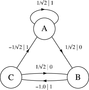
Figure 1: The Golden Mean quantum generator.

The process language generated by this QFG is the so-called Golden-Mean Process language [1]. The word distribution is shown in Fig. 2. It is characterized by the set of irreducible forbidden words $\mathcal{F}=\{00\}$: no consecutive zeros occur. In other words, for the spin-$1$ particle the spin component along the $y$-axis never vanishes twice in a row. This restriction—the dominant structure in the process—is a short-range correlation since the measurement outcome at time $t$ only depends on the immediately preceding one at time $t-1$. If the outcome is $0$, the next outcome will be $1$ with certainty. If the outcome is $1$, the next measurement is maximally uncertain: outcomes $0$ and $1$ occur with equal probability.

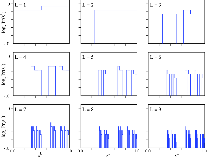
Figure 2: Golden Mean process language: Word $\{00\}$ has zero probability; all others have nonzero probability. The logarithm base 2 of the word probabilities is plotted versus the binary string $s^{L}$, represented as base-$2$ real number “$0.s^{L}$”. To allow word probabilities to be compared at different lengths, the distribution is normalized on $[0,1]$—that is, the probabilities are calculated as densities.

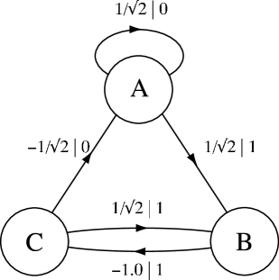
Figure 3: The Even Process quantum generator.

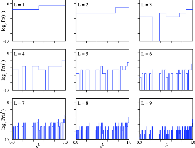
Figure 4: Even Process language: Words $\{01^{2k-1}0\},k=1,2,3,...$ have zero probability; all others have nonzero probability.

Consider the same Hamiltonian, but now use instead the observable $J_{x}^{2}$. The corresponding projection operators define the QFG:

$$P(0) =\mathinner{|{100}\rangle}\mathinner{\langle{100}|}$$

$$~{}\mathrm{and}~{}~{}P(1) =\mathinner{|{010}\rangle}\mathinner{\langle{010}|}+\mathinner{|{001}\rangle}\mathinner{\langle{001}|}~{}.$$ (18)

The QFG defined by $U$ and these projection operators is shown in Fig. 3. The process language generated by this QFG is the so-called Even Process language [21, 1]. The word distribution is shown in Fig. 4. It is defined by the infinite set of irreducible forbidden words $\mathcal{F}=\{01^{2k-1}0\},k=1,2,3,...$. That is, if the spin component equals 0 along the $x$-axis it will be zero an even number of consecutive measurements before being observed to be nonzero. This is a type of infinite correlation: For a possibly infinite number of time steps the system tracks the evenness or oddness of number of consecutive measurements of “spin component equals 0 along the $x$-axis”.

Note that changing the measurement, specifically choosing $J_{z}^{2}$ as the observable, yields a QFG that generates Golden Mean process language again.

The two processes produced by these quantum dynamical systems are well known in the context of symbolic dynamics [5]—a connection we will return to shortly. Let us first, though, turn to another important property of finite-state machines and explore its role in computational capacity and dynamics.

IV Determinism

The label determinism is used in a variety of senses, some of which are seemingly contradictory. Here, we adopt the notion, familiar from automata theory [6], which differs from that in physics, say, of non-stochasticity. One calls a finite-state machine (classical or quantum) deterministic whenever the transition from one state to the next is uniquely determined by the output symbol, or input symbol for recognizers. It is important to realize that a deterministic finite-state machine can still behave stochastically—stochasticity here referring to the positive probability of generating symbols. Once the symbol is determined, though, the transition taken by the machine to the next state is unique. Thus, what is called a stochastic process in dynamical systems theory can be described by a deterministic finite-state generator without contradiction.

We can easily check the two quantum finite-state machines in Figs. 1 and 3 for determinism by inspecting each state and its outgoing transitions. One quickly sees that both generators are deterministic. In contrast, the third QFG mentioned above, defined by $U$ in Eq. (5) and $J_{z}^{2}$, is nondeterministic.

Determinism is a desirable property for various reasons. One is the simplicity of the mapping between observed symbols and internal states. Once the observer synchronizes to the internal state dynamics, the output symbols map one-to-one onto the internal states. In general, though, the observed symbol sequences do not track the internal state dynamics (orbit) directly. (This brings one to the topic of hidden Markov chains [22].)

For optimal prediction, however, access to the internal state dynamics is key. Thus, when one has a deterministic model, the observed sequences reveal the internal dynamics. Once they are known and one is synchronized, the process becomes optimally predictable. A final, related reason why determinism is desirable is that closed-form expressions can be given for various information processing measures, as we will discuss in Sec. VI.

V Sofic systems

In symbolic dynamics, sofic systems are used as tractable representations with which to analyze continuous-state dynamical systems [5, 1]. Let the alphabet ${\mathcal{A}}$ together with an $n\times n$ adjacency matrix (with entries $0$ or $1$) define a directed graph $G=(V,E)$ with $V$ the set of vertices and $E$ the set of edges. Let $X$ be the set of all infinite admissible sequences of edges, where admissible means that the sequence corresponds to a path through the graph. Let $T$ be the shift operator on this sequence; it plays the role of the time-evolution operator of the dynamical system. A sofic system is then defined as the pair $(X,T)$ [23]. The Golden Mean and the Even process are standard examples of sofic systems. The Even system, in particular, was introduced by Hirsch et al in the 1970s [21].

Whenever the rule set for admissible sequences is finite one speaks of a subshift of finite type. The Golden Mean process is a subshift of finite type. Words in the language are defined by the finite (single) rule of not containing the subword $00$. The Even Process, on the other hand, is not of finite type, since the number of rules is infinite: The forbidden words $\{01^{2k+1}0\}$ cannot be reduced to a finite set. As we noted, the rule set, which determines allowable words, implies the process has a kind of infinite memory. One refers, in this case, to a strictly sofic system.

The spin-$1$ example above appears to be the first time a strictly sofic system has been identified in quantum dynamics. This ties quantum dynamics to languages and quantum automata theory in a way similar to that found in classical dynamical systems theory. In the latter setting, words in the sequences generated by sofic systems correspond to regular languages—languages recognized by some finite-state machine. We now have a similar construction for quantum dynamics. For any (finite-dimensional) quantum dynamical system under observation we can construct a QFG, using a unitary operator and a set of projection operators. The language it generates can then be analyzed in terms of the rule set of admissible sequences. One interesting open problem becomes the question whether the words produced by sofic quantum dynamical systems correspond to the regular languages. An indication that this is not so is given by the fact that finite-state quantum recognizers can accept nonregular process languages [11].

VI Information-theoretic analysis

The process languages generated by the spin-$1$ particle under a particular observation scheme can be analyzed using well known information-theoretic quantities such as Shannon block entropy and entropy rate [12] and others introduced in Ref. [24]. Here, we will limit ourselves to the excess entropy. The applicability of this analysis to quantum dynamical systems has been shown in Ref. [25], where closed-form expressions are given for some of these quantities when the generator is known.

We can use the observed behavior, as reflected in the word distribution, to come to a number of conclusions about how a quantum process generates randomness and stores and transforms historical information. The Shannon entropy of length-$L$ sequences is defined

$$H(L) \equiv-\sum_{s^{L}\in{\cal A}^{L}}\mathrm{Pr}(s^{L}){\rm log}_{2}\mathrm{Pr}(s^{L})~{}.$$ (19)

It measures the average surprise in observing the “event” $s^{L}$. Ref. [24] showed that a stochastic process’s informational properties can be derived systematically by taking derivatives and then integrals of $H(L)$, as a function of $L$. For example, the source entropy rate $h_{\mu}$ is the rate of increase with respect to $L$ of the Shannon entropy in the large-$L$ limit:

$$h_{\mu}\equiv\lim_{L\rightarrow\infty}\left[H(L)-H(L-1)\right]\;,$$ (20)

where the units are bits/measurement [12].

Ref. [25] showed that the entropy rate of a quantum process can be calculated directly from its QFG, when the latter is deterministic. A closed-form expression for the entropy rate in this case is given by:

$$h_{\mu}=-|Q|^{-1}\sum_{i=0}^{|Q|-1}\sum_{j=0}^{|Q|-1}|U_{ij}|^{2}\log_{2}|U_{ij}|^{2}~{},$$ (21)

The entropy rate $h_{\mu}$ quantifies the irreducible randomness in processes: the randomness that remains after the correlations and structures in longer and longer sequences are taken into account.

The latter, in turn, is measured by a complementary quantity. The amount $I(\stackrel{{\scriptstyle\leftarrow}}{{S}};\stackrel{{\scriptstyle\rightarrow}}{{S}})$ of mutual information [12] shared between a process’s past $\stackrel{{\scriptstyle\leftarrow}}{{S}}$ and its future $\stackrel{{\scriptstyle\rightarrow}}{{S}}$ is given by the excess entropy ${\bf E}$ [24]. It is the subextensive part of $H(L)$:

$${\bf E}=\lim_{L\rightarrow\infty}[H(L)-h_{\mu}L]\;.$$ (22)

Note that the units here are bits.

Ref. [24] gives a closed-form expression for ${\bf E}$ for order-$R$ Markov processes—those in which the measurement symbol probabilities depend only on the previous $R-1$ symbols. In this case, Eq. (22) reduces to:

$$E=H(R)-R\cdot h_{\mu}~{},$$ (23)

where $H(R)$ is a sum over $|{\mathcal{A}}|^{R}$ terms. Given that the quantum generator is deterministic we can simply employ the above formula for $h_{\mu}$ and compute the block entropy at length $R$ to obtain the excess entropy for the order-$R$ quantum process.

Ref. [25] computes these entropy measures for various example systems, including the spin-$1$ particle. The results are summarized in Table 1. The value for the excess entropy of the Golden Mean process obtained by using Eq. (23) agrees with the value obtained from simulation data, shown in Table 1. The entropy $h_{\mu}=2/3$ bits per measurement for both processes, and thus they have the same amount of irreducible randomness. The excess entropy, though, differs markedly. The Golden Mean process ($J_{y}^{2}$ measured) stores, on average, ${\bf E}\approx 0.25$ bits at any given time step. The Even Process ($J_{x}^{2}$ measured) stores, on average, ${\bf E}\approx 0.90$ bits, which reflects its longer memory of previous measurements.

Quantum	Spin-1
Dynamical System	Particle
Observable	$J_{y}^{2}$	$J_{x}^{2}$
$h_{\mu}$ [bits/measurement]	0.666	0.666
${\bf E}$ [bits]	0.252	0.902

Table 1: Information storage and generation for example quantum processes: entropy rate $h_{\mu}$ and excess entropy ${\bf E}$.

VII Conclusion

We have shown that quantum dynamical systems store information in their dynamics. The information is accessed via measurement. Closer inspection would suggest even that information is created through measurement. In any case, the key conclusion is that, since both processes are represented by a $3$-state QFG constructed from the same internal quantum dynamics, it is the means of observation alone that affects the amount of memory. This was illustrated with the particular examples of the spin-$1$ particle in a magnetic field. Depending on the choice of observable the spin-$1$ particle generates different process languages. We showed that these could be analyzed in terms of the block entropy—a measure of uncertainty, the entropy rate—a measure of irreducible randomness, and the excess entropy—a measure of structure. Knowing the (deterministic) QFG representation, these quantities can be calculated in closed form.

We established a connection between quantum automata theory and quantum dynamics, similar to the way symbolic dynamics connects classical dynamics and automata. By considering the output sequence of a repeatedly measured quantum system as a shift system we found quantum processes that are sofic systems. Taking one quantum system and observing it in one way yields a subshift of finite type. Observing it in a different way yields a (strictly sofic) subshift of infinite type. Consequently, not only the amount of memory but also the soficity of a quantum process depend on the means of observation.

This can be compared to the fact that, classically the Golden Mean and the Even sofic systems can be transformed into each other by a two-block map. The adjacency matrix of the graphs is the same. A similar situation arises here. The unitary matrix, which is the corresponding adjacency matrix of the quantum graph, is the same for both processes. The processes can be transformed into each other by expressing one set of projection operators in the eigenbasis of the other. This transformation always exists since the operators simply represent different orthonormal basis sets spanning the Hilbert space.

The preceding attempted to forge a link between quantum dynamical systems and quantum computation by extending concepts from symbolic dynamics to the quantum setting. We believe the results suggest further study of the properties of quantum finite-state generators and the processes they generate is necessary and will shed light on a number of questions in quantum information processing. One open technical question is whether sofic quantum systems are the closure of quantum subshifts of finite-type, as they are for classical systems [23]. There are indications that this is not so. For example, as we noted, quantum finite-state recognizers can recognize nonregular process languages [11].

References

- [1] B. P. Kitchens. Symbolic dynamics: one-sides, two-sided, and countable state Markov shifts. Springer Verlag, Berlin Heidelberg, 1998.
- [2] G. H. Hedlund and M. Morse. Symbolic dynamics i. Amer. J. Math., 60:815–866, 1938.
- [3] G. H. Hedlund and M. Morse. Symbolic dynamics ii. Amer. J. Math., 62:1–42, 1940.
- [4] C. E. Shannon and W. Weaver. The Mathematical Theory of Communication. University of Illinois Press, Champaign-Urbana, 1962.
- [5] D. Lind and B. Marcus. An introduction to symbolic dynamics and coding. Cambridge University Press, 1995.
- [6] J. E. Hopcroft, R. Motwani, and J. D. Ullman. Introduction to Automata Theory, Languages, and Computation. Addison-Wesley, 2001.
- [7] M. C. Gutzwiller. Chaos in Classical and Quantum Mechanics. Springer Verlag, 1990.
- [8] L. E. Reichl. The transition to chaos: Conservative classical systems and quantum manifestations. Springer, New York, 2004.
- [9] S. Habib, K. Jacobs, and K. Shizume. Emergence of chaos in quantum systems far from the classical limit. Phys. Rev. Lett., 96:010403–06, 2006.
- [10] R. Alicki and M. Fannes. Quantum dynamical systems. Oxford University Press, 2001.
- [11] K. Wiesner and J. P. Crutchfield. Computation in finitary quantum processes. submitted, e-print arxiv/quant-ph/0608206, 2006.
- [12] T. Cover and J. Thomas. Elements of Information Theory. Wiley-Interscience, 1991.
- [13] D. Z. Albert. On quantum-mechanical automata. Physics Letters, 98A:249–251, 1983.
- [14] A. Peres. On quantum-mechanical automata. Physics Letters, 101A:249–250, 1984.
- [15] C. Moore and J. P. Crutchfield. Quantum automata and quantum grammars. Theor. Comp. Sci., 237:275–306, 2000.
- [16] A. Kondacs and J. Watrous. On the power of quantum finite state automata. In 38th IEEE Conference on Foundations of Computer Science, pages 66–75, 1997.
- [17] D. Aharonov, A. Kitaev, and N. Nisan. Quantum circiuts with mixed states. In 30th Annual ACM Symposium on the Theory of Computing, pages 20–30, 1998.
- [18] A. Ambainis and J. Watrous. Two-way finite automata with quantum and classical states. Theoretical Computer Science, 287:299–311, 2002.
- [19] R. Freivalds and A. Winter. Quantum finite state transducers. Lect. Notes Comp. Sci., 2234:233–242, 2001.
- [20] A. Peres. Quantum theory: concepts and methods. Kluwer Academic Publishers, Dordrecht, 1993.
- [21] M. Hirsch, J. Palis, C. Pugh, and M. Shu. Neighborhoods of hyperbolic sets. Inventiones Math., 9:121–134, 1970.
- [22] C. M. Bishop. Pattern recognition and machine learning. Springer Verlag, Singapore, 2006.
- [23] B. Weiss. Subshifts of finite type and sofic systems. Monatshefte für Mathematik, 77:462–474, 1973.
- [24] J. P. Crutchfield and D. P. Feldman. Regularities unseen, randomness observed: Levels of entropy convergence. Chaos, 13:25 – 54, 2003.
- [25] J. P. Crutchfield and K. Wiesner. Intrinsic quantum computation. submitted, e-print arxiv/quant-ph/0611202, 2006.