Pulse shapes from electron and photon induced events in segmented high-purity germanium detectors

Abstract

Experiments built to search for neutrinoless double beta-decay are limited in their sensitivity not only by the exposure but also by the amount of background encountered. Radioactive isotopes in the surrounding of the detectors which emit gamma-radiation are expected to be a significant source of background in the GERmanium Detector Array, GERDA.

Methods to select electron induced events and discriminate against photon induced events inside a germanium detector are presented in this paper. The methods are based on the analysis of the time structure of the detector response. Data were taken with a segmented GERDA prototype detector. It is shown that the analysis of the time response of the detector can be used to distinguish multiply scattered photons from electrons.

, , , , ,

1 Introduction

Radioactive decays in which photons with energies above $Q=2039$ keV are emitted are expected to be a significant source of background for the GERmanium Detector Array, GERDA [1]. GERDA is an experiment which is currently being constructed and has as aim the search for the neutrinoless double beta-decay ($0\nu\beta\beta$) of the germanium isotope ⁷⁶Ge.

Methods to distinguish between electrons and multiply scattered photons using the time structure of the germanium detector response, or pulse shape, are presented in this paper. The pulse shape depends on the location and the spatial distribution over which energy is deposited inside the detector in a single event. Photons in the MeV-energy region will predominantly Compton-scatter and deposit energy at locations separated by centimeters. These events are referred to as multi-site events. In contrast, electrons in the same energy region have a range of the order of a millimeter. Events of this kind are referred to as single-site events.

Pulse shape analysis methods have been developed for nuclear experiments such as AGATA [2] and GRETA [3] as well as for double beta-decay experiments [4, 5, 6, 8, 9]. In the context of the latter these techniques are now extended to segmented detectors. In this study the focus is on the pulse shape analysis after the application of a single segment requirement as presented in [10]. The performance of the pulse shape analysis with and without segment information is compared based on data taken with an 18-fold segmented GERDA prototype detector.

The experimental setup and the collected data sets are described in Section 2. The accompanying Monte Carlo simulation is introduced in Section 3. A parameter accessible in simulations which is a measure of the volume over which energy is deposited inside the detector is defined. A definition of single-site and multi-site events is derived from the Monte Carlo data sets based on this parameter. The fraction of single-site and multi-site events in the data sets is estimated. Three analysis methods are presented in Section 4 and these methods are applied to the data sets taken with the prototype detector. The results are summarized in Section 5. Conclusions are drawn in Section 6.

2 Experimental setup and data sets

2.1 Experimental setup and data taking

The segmented germanium detector under study is the first segmented GERDA prototype detector. The true coaxial cylindrical crystal has a height of 70 mm, an outer diameter of 70 mm and a central bore with a diameter of 10 mm. It is 18-fold segmented with a 6-fold segmentation in the azimuthal angle $\phi$ and a 3-fold segmentation in the height $z$. It was operated in a conventional test cryostat. Signals from the core and the segment electrodes were amplified and subsequently digitized using a 14-bit ADC with a sampling rate of 75 MHz. The energy and the pulse shapes of the core and the 18 segment electrodes were recorded for each event. The pulse shape data consists of 300 13.3 ns samples of the integrated charge amplitude. The onset of the signal was delayed by one $\mu$s. The (full width at half maximum) energy resolution of the core electrode was 2.6 keV at energies around 1.3 MeV, the energy resolutions of the segment electrodes ranged from 2.4 keV to 4.8 keV with an average segment energy resolution of 3.3 keV. Details of the experimental setup and the detector performance can be found in [11].

A 100 kBq ²²⁸Th source was placed at $z=0$ cm and $r=17.5$ cm with respect to the detector center ($z=0$ cm, $r=0$ cm) facing towards the center of a segment, $S$, located in the middle row. Two data sets were taken with different trigger conditions labeled $TR_{C}$ and $TR_{S}$. The former trigger condition requires the core electrode to show an energy above 1 MeV. The collected data set is referred to as core data set and contains $127\,000$ events. The latter trigger condition requires segment $S$ to show an energy above 1 MeV. 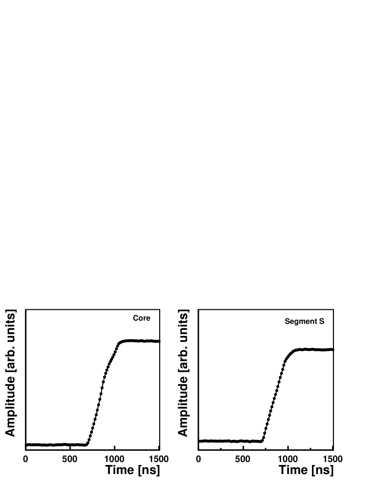The collected data set is referred to as segment data set and contains $420\,000$ events. As an example, Figure 1 shows a pulse shape measured with the core (left) and with the segment $S$ electrode (right) for an event in the segment data set. The core-energy spectra will be shown in Section 5.3.

Figure 1: Pulse shape measured with the core (left) and with the segment $S$ electrodes (right) for an event in the segment data set. The energy of $1758$ keV seen in the core is completely contained in segment $S$. The starting time is chosen arbitrarily in this example. The amplitude is in arbitrary units but the scale is the same for both pulse shapes. The pulse shapes are dominated by different charge carrier types.

2.2 Event selection

A pre-selection applied to the segment data set collects events with energy deposited only in one segment. It requires the energy measured in segment $S$ to be the same as the energy measured in the core within $\pm 5$ keV, according to about $\pm 4~{}\sigma$ given the energy resolution. In total, $150\,396$ events fulfill the pre-selection criterion.

Four data samples each are selected from the core and segment data sets. The data samples are defined by the energy measured in the core and are labeled:

• $DEP$: The sample contains events with a core energy in the region of $(1593\pm 5)$ keV. These events are associated with the double escape peak of the $2615$ keV ²⁰⁸Tl photon. The photon produces electron-positron pairs of which the positron subsequently annihilates. Both 511 keV annihilation photons escape the detector. The energy is predominantly deposited on a millimeter-scale; i.e., locally.

• $\Gamma_{1}$: The sample contains events with a core energy in the region of $(1620\pm 5)$ keV. These events are associated with photons of this energy produced in the decay of ²¹²Bi. The photons mostly scatter multiple times before their energy is fully deposited inside the detector.

• $\Gamma_{2}$: The sample contains events with a core energy in the region of $(2615\pm 5)$ keV. These events are associated with photons of this energy produced in the decay of ²⁰⁸Tl. The photons mostly scatter multiple times before their energy is fully deposited inside the detector.

• $ROI$: The sample contains events with a core energy in the region of interest, $(2039\pm 50)$ keV. These events are predominantly associated with Compton-scattered photons from ²⁰⁸Tl.

The requirements of the trigger, pre-selection and event selection are listed in Table 1. Also the number of events in the corresponding data samples are shown. The amount of background in each data sample, as estimated from taking spectra without the ²²⁸Th source present, was found to be less than 1%.

Table 1: Requirements of the trigger, pre-selection and event selection, and the number of events in the corresponding data samples. $E_{C}$ and $E_{S}$ are the energies seen in the core and in segment $S$, respectively.

Cut	Condition	Events
Trigger ($TR_{C}$)	$E_{C}>1$ MeV	$127\,000$
Pre-selection	-	$127\,000$
Selection ($DEP$)	$\left|E_{C}-1593\mathrm{~{}keV}\right|<\phantom{0}5$ keV	$1673$
Selection ($\Gamma_{1}$)	$\left|E_{C}-1620\mathrm{~{}keV}\right|<\phantom{0}5$ keV	$1965$
Selection ($\Gamma_{2}$)	$\left|E_{C}-2615\mathrm{~{}keV}\right|<\phantom{0}5$ keV	$22\,924$
Selection ($ROI$)	$\left|E_{C}-2039\mathrm{~{}keV}\right|<50$ keV	$6\,431$
Trigger ($TR_{S}$)	$E_{S}>1$ MeV	$420\,000$
Pre-selection	$\left|E_{C}-E_{S}\right|<5$ keV	$150\,396$
Selection ($DEP$)	$\left|E_{C}-1593\mathrm{~{}keV}\right|<\phantom{0}5$ keV	$3492$
Selection ($\Gamma_{1}$)	$\left|E_{C}-1620\mathrm{~{}keV}\right|<\phantom{0}5$ keV	$1972$
Selection ($\Gamma_{2}$)	$\left|E_{C}-2615\mathrm{~{}keV}\right|<\phantom{0}5$ keV	$19\,243$
Selection ($ROI$)	$\left|E_{C}-2039\mathrm{~{}keV}\right|<50$ keV	$7707$

3 Monte Carlo simulation

The GEANT4 [12] based MaGe [13] framework was used to simulate the prototype detector setup (for details and a validation of this particular simulation see [10]). A Monte Carlo study was performed to estimate the spatial distribution over which energy is deposited in the detector for events in the different data samples. A ²²⁸Th source was simulated. The trigger, pre-selection and event selection requirements discussed in the previous section were applied to the Monte Carlo data. The data sets are referred to as core and segment Monte Carlo data sets.

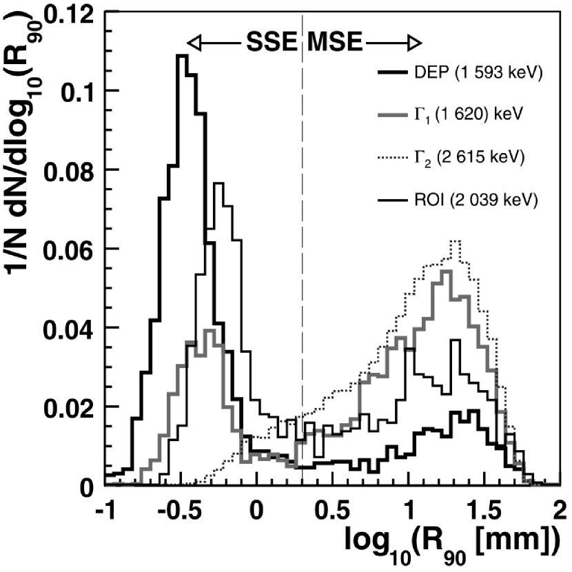
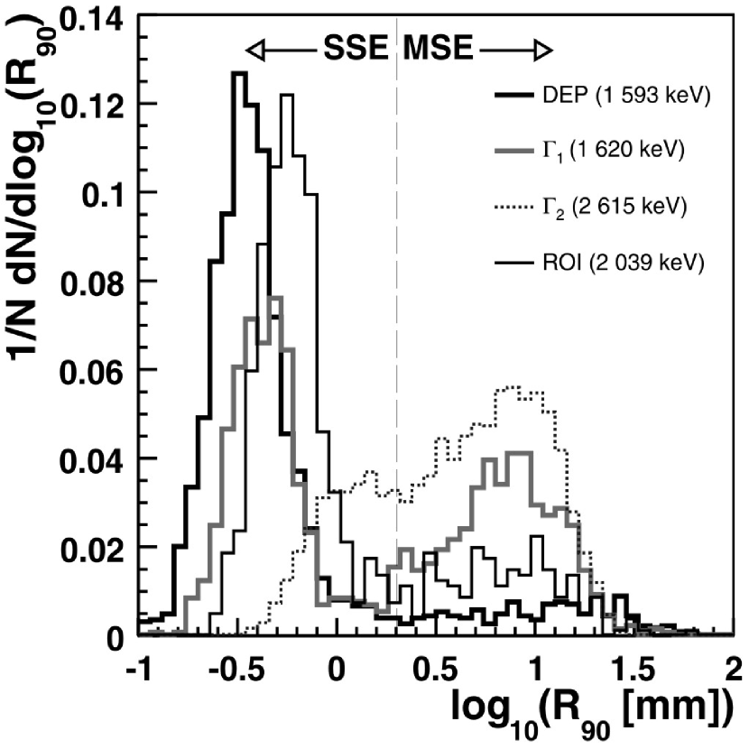
A measure for the spatial distribution over which energy is distributed inside the detector is the radius $R_{90}$. This is defined as the radius inside which 90% of the energy in a single event is deposited; for a detailed discussion see [7]. Figure 2 shows the distribution of $R_{90}$ for the $DEP$, $\Gamma_{1}$, $\Gamma_{2}$ and $ROI$ samples for the core (left) and segment (right) Monte Carlo data sets. All distributions are normalized to unity. The $R_{90}$ distributions range from 0.1 mm ($\log_{10}(R_{90})=-1$) up to 7 cm ($\log_{10}(R_{90})=1.8$). The $DEP$ samples are dominated by events with $R_{90}$ in a region from 0.1 mm to 1 mm. A long tail towards larger radii is visible and mostly due to events in the underlying Compton-shoulder of ²⁰⁸Tl and events in which electrons undergo hard bremsstrahlung processes. The $R_{90}$ distributions for the $\Gamma_{1}$ and $ROI$ samples have two prominent regions each, one at radii from 0.3 mm to 1 mm and a second from 3 mm to 6 cm. The latter one is due to multiply scattered photons whereas the former is due to photons with higher energy which only scatter once and then leave the detector. The $R_{90}$ distributions for the $\Gamma_{2}$ samples range from 0.3 mm to about 7 cm with a maximum at around 2 cm for the core Monte Carlo data sample and at around 1 cm for the segment Monte Carlo data sample. The sample is dominated by events in which photons scatter multiple times. No peak at small $R_{90}$ is visible.

It is expected that the single segment requirement rejects events with large values of $R_{90}$. Indeed, the distributions of $R_{90}$ in the segment Monte Carlo data samples are suppressed in the region above 1 cm. The peaks between 0.1 mm and 1 mm in the $DEP$, $\Gamma_{1}$ and $ROI$ samples are more pronounced in this case.

Figure 2: Normalized distributions of $R_{90}$ for the $DEP$, $\Gamma_{1}$, $\Gamma_{2}$ and $ROI$ samples for the Monte Carlo core (left) and segment data sets (right). Single-site events (SSE) and multi-site events (MSE) are defined by requiring $R_{90}<2$ mm and $R_{90}>2$ mm (dashed line) as discussed in the text.

Single-site and multi-site events are defined by requiring $R_{90}<\overline{R}$ and $R_{90}>\overline{R}$, respectively, where $\overline{R}$ is a chosen parameter value. The distributions of $R_{90}$ for the $DEP$ samples suggest $\overline{R}=2$ mm ($\log_{10}(\overline{R})=0.3$). Also, due to the sampling rate of 75 MHz and the average drift velocity of charge carriers ($\mathcal{O}(10^{8})$ mm/s) energy deposits closer than about 2 mm cannot be resolved. The fractions of single-site events in the Monte Carlo data samples are thus defined and summarized in Table 2. Also listed are the corresponding systematic uncertainties of the fractions which are derived by varying the parameter $\overline{R}$ by $\pm 1$ mm.

Table 2: Fractions of single-site events in the Monte Carlo data samples. The errors are derived by varying the parameter $\overline{R}$ by $\pm 1$ mm.

Monte Carlo data samples	$DEP$	$\Gamma_{1}$	$\Gamma_{2}$	$ROI$
	($1593$ keV)	($1620$ keV)	($2615$ keV)	(2039 keV)
Core samples	$(77.9^{+1.6}_{-3.4})$%	$(30.5^{+4.0}_{-3.6})$%	$(12.2^{+\phantom{0}6.0}_{-\phantom{0}7.6})$%	$(52.4^{+3.8}_{-7.6})$%
Segment samples	$(89.0^{+1.1}_{-3.0})$%	$(55.0^{+5.0}_{-4.4})$%	$(30.0^{+10.0}_{-16.8})$%	$(77.6^{+3.4}_{-6.7})$%

The Monte Carlo data samples are not purely composed of single-site or multi-site events. The $DEP$ samples are dominated by single-site events, the $\Gamma_{1}$ and $\Gamma_{2}$ have large fractions of multi-site events. Events in the $DEP$ samples are referred to as electron-like while events in the $\Gamma_{1}$ and $\Gamma_{2}$ samples are referred to as photon-like in the following. Note, that these two labels do not describe an intrinsic property of an event (such as the range of energy deposition), but they are used to emphasize the different probabilities of the event being single-site or multi-site.

4 Analysis methods

Three analysis methods were tested. Half of the $DEP$ and $\Gamma_{1}$ data samples were used to train the methods. The other half of the samples, together with the $\Gamma_{2}$ and $ROI$ samples, were used to test the analysis methods. The $DEP$ and $\Gamma_{1}$ samples were selected for training in order to avoid biases due to the difference in energy of events in the two samples. For the same reason the maximum of each pulse shape was normalized to unity for each event.

The analyses were applied to the core and segment data samples in order to study the effect of pulse shape analysis before and after the application of a single segment requirement. In the former case, only the core pulse shape was used. In the latter case, the core pulse shape was used and, optionally, the segment $S$ pulse shape in addition.

4.1 Likelihood discriminant method

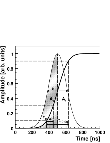
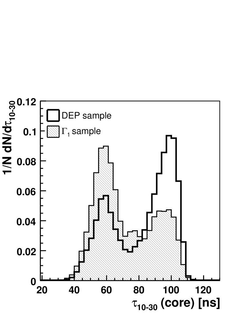
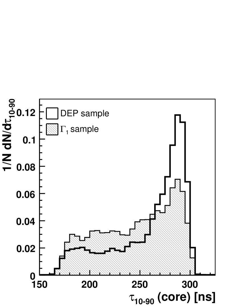
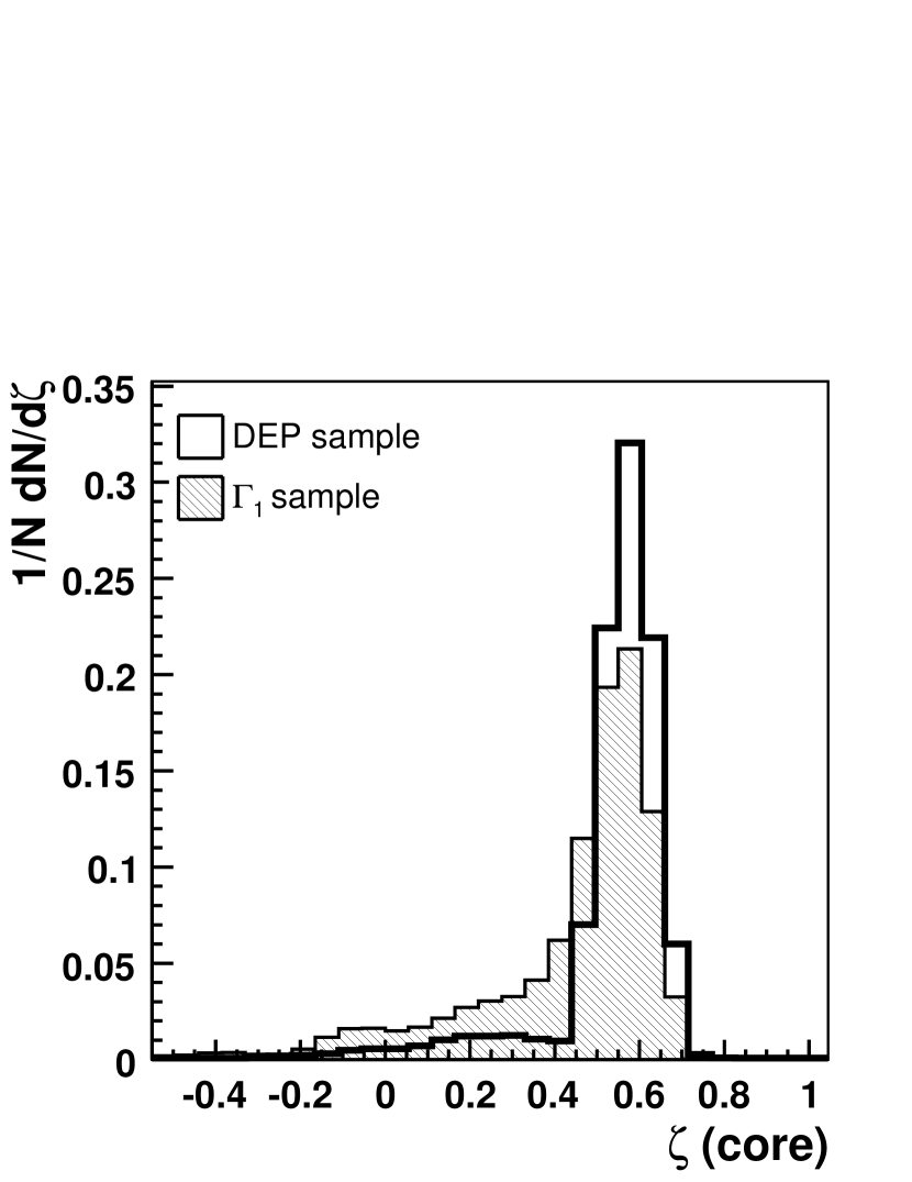
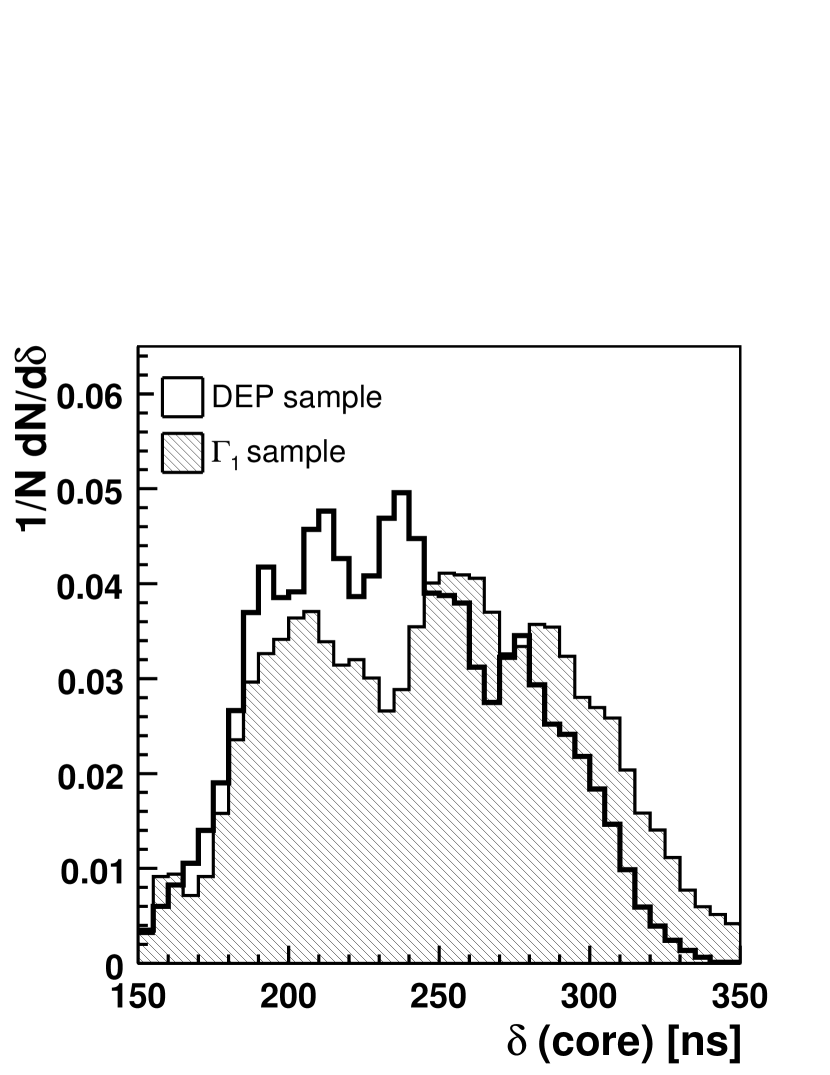
Four quantities are calculated for each pulse shape. These quantities provided separation power in previous studies [8, 9]. Interpolation algorithms were applied to the pulse shapes to obtain continuous distributions. Figure 3 shows an ideal pulse and the quantities calculated are indicated. All quantities are given subscripts $C$ and $S$ for the core and segment pulse shapes, respectively.

• Risetime $\tau_{10-30}$, defined as the difference between the times the integrated charge amplitude has reached 10% and 30% of its maximal amplitude;

• risetime $\tau_{10-90}$, defined as the difference between the times the integrated charge amplitude has reached 10% and 90% of its maximal amplitude;

• left-right asymmetry $\zeta$, defined as the asymmetry of the area below the left and the right half of the current pulse, $A_{l}$ and $A_{r}$, measured from the maximum, $\zeta=\frac{A_{l}-A_{r}}{A_{l}+A_{r}}$;

• current pulse width $\delta$, defined as the full width at half maximum of the current pulse.

Figure 3: Ideal pulse shape: the integrated charge (thick line) and the current (thin line). Indicated are the quantities $\tau_{10-30}$, $\tau_{10-90}$, $\delta$, $A_{l}$ and $A_{r}$ (see text).

The variables are histogrammed for both training samples and their integrals are normalized to unity. As an example, Figure 4 shows the normalized distributions of the four quantities calculated from the core pulse shape in the two segment data samples. The average risetime of pulses in the $DEP$ sample is larger than that of pulses in the $\Gamma_{1}$ sample . The relative frequencies are used to define discriminants, given that the event is electron-like ($DEP$ sample) or photon-like ($\Gamma_{1}$ sample). The respective overall discriminants, $p_{e^{-}}$ and $p_{\gamma}$, are calculated by multiplying the individual discriminants:

$$p_{e^{-}}^{k} = p(\tau_{\mathrm{10-30},k}|e^{-})\cdot p(\tau_{\mathrm{10-90},k}|e^{-})\cdot p(\zeta_{k}|e^{-})\cdot p(\delta_{k}|e^{-})\ ,$$ (1)

$$p_{\gamma}^{k} = p(\tau_{\mathrm{10-30},k}|\gamma)\cdot p(\tau_{\mathrm{10-90},k}|\gamma)\cdot p(\zeta_{k}|\gamma)\cdot p(\delta_{k}|\gamma)\ ,$$ (2)

with $k=C$ or $S$ for the core and segment pulses, respectively. Note that no correlations among these quantities are taken into account.

Likelihood discriminants (LHD) are constructed from $p_{e^{-}}$ and $p_{\gamma}$ for each individual event:

$$D^{C} = \frac{p_{e^{-}}^{C}}{p_{e^{-}}^{C}+p_{\gamma}^{C}}\ ,$$ (3)

$$D^{C+S} = \frac{p_{e^{-}}^{C}\cdot p_{e^{-}}^{S}}{p_{e^{-}}^{C}\cdot p_{e^{-}}^{S}+p_{\gamma}^{C}\cdot p_{\gamma}^{S}}\ ,$$ (4)

where $D^{C}$ uses information from the core electrode only and $D^{C+S}$ uses information from the core and segment electrodes. $D$ varies between 0 and 1 by construction. $D$ peaks at 1 for electron-like events; for photon-like events $D$ peaks at 0. Events are identified as electron-like for $D>\overline{D}$ and as photon-like for $D<\overline{D}$, where $\overline{D}$ is a chosen parameter.

Figure 4: Quantities calculated from the core pulseshapes in the $DEP$ (open histogram) and $\Gamma_{1}$ (hatched histogram) segment data samples. Top left: risetime $\tau_{10-30}$, top right: risetime $\tau_{10-90}$, bottom left: left-right asymmetry $\zeta$, bottom right: current pulse width $\delta$.

4.2 Library method

The training $DEP$ samples are interpreted as libraries of electron-like reference pulses. An average $\chi^{2}$ with respect to all reference pulses is calculated for each pulse shape in the test samples. For the $k$th reference pulse and the $l$th pulse shape under study the average $\chi^{2}$ is defined as

$$\chi_{k,l}^{2}=\frac{1}{N}\sum_{i=1}^{N}\frac{(x_{k,i}-x_{l,i})^{2}}{\sigma^{2}}\ ,$$ (5)

where $N$ is the number of bins of the pulse shapes and $x_{k,i}$ and $x_{l,i}$ are the pulse heights in bin $i$ of the $k$th reference pulse and the $l$th pulse under study. $\sigma^{2}$ is defined as

$$\sigma^{2}=\sigma_{\mathrm{k}}^{2}+\sigma_{\mathrm{l}}^{2},$$ (6)

where $\sigma_{\mathrm{k}}$ and $\sigma_{\mathrm{l}}$ are the noise amplitudes of the reference pulse shape and the pulse shape under study. The noise amplitude is the RMS of the baseline measured during the one $\mu$s before the onset of the pulse.

The minimum $\chi^{2}$ is selected with respect to the reference pulses and denoted $\chi^{2}_{\mathrm{min}}=\chi^{2}_{k_{\mathrm{min}},l}$ for each pulse shape in the test sample. Ideally, the minimum $\chi^{2}$ for electron-like events should be smaller than that of photon-like events. Events are identified as electron-like for $\chi^{2}_{\mathrm{min}}<\overline{\chi^{2}}$ and as photon-like for $\chi^{2}_{\mathrm{min}}>\overline{\chi^{2}}$, where $\overline{\chi^{2}}$ is a chosen parameter.

4.3 Neural network method

Artificial neural networks (ANNs) are used to separate electron-like from photon-like events. Input neurons are fed with samples of the normalized pulse shape, starting from the time when the amplitude has reached 10%. 40 consecutive samples per pulse shape are used. The ANN consists of 40 input neurons, 40 hidden neurons and one output neuron for the core data samples. An additional 40 input neurons are used optionally for the segment data samples.

The ANNs are trained by feeding them with pulse shapes from the two training samples and simultaneously providing the information which of the samples each pulse belongs to (0: $DEP$ sample, 1: $\Gamma_{1}$ sample). The ANNs adjust the internal neurons iteratively using the Broyden, Fletcher, Goldfarb, Shanno (BFGS) learning method [14]. Each ANN is trained in about $1000$ iterations. The output quantity, $NN$, is on average larger for photon-like events than for electron-like events. Events are identified as electron-like for $NN<\overline{NN}$ and as photon-like for $NN>\overline{NN}$, where $\overline{NN}$ is a chosen parameter.

5 Results

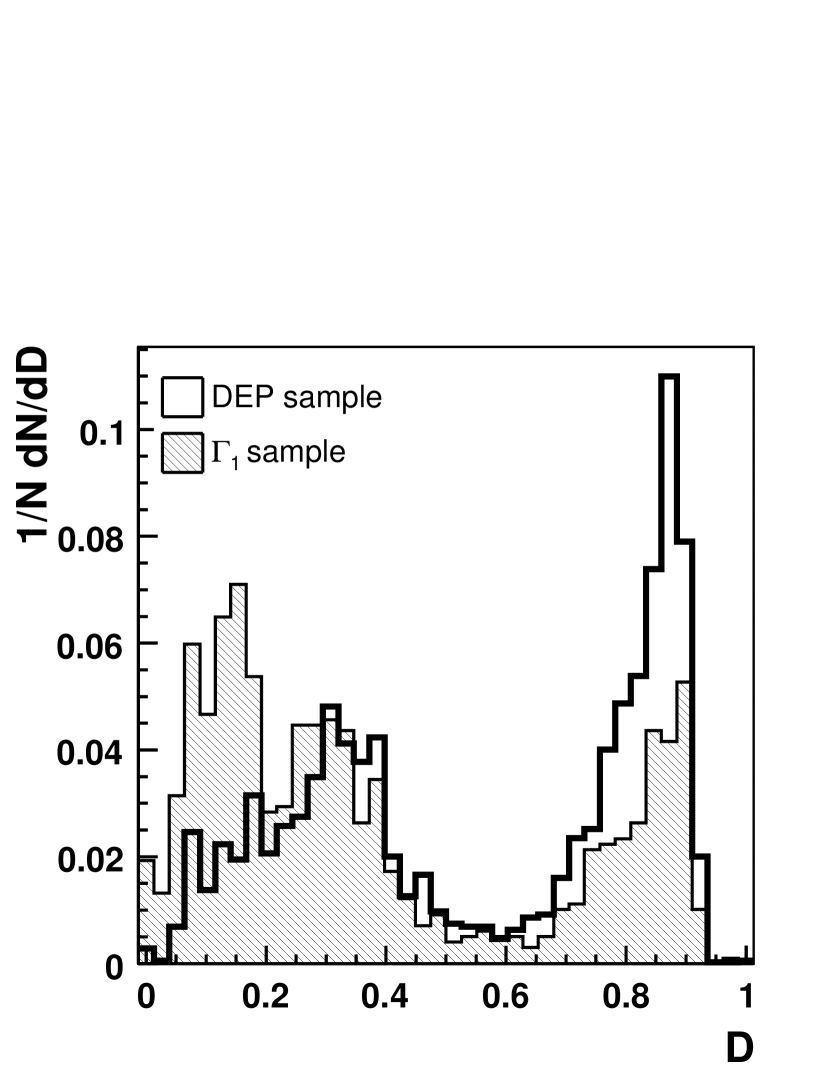
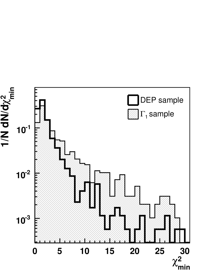
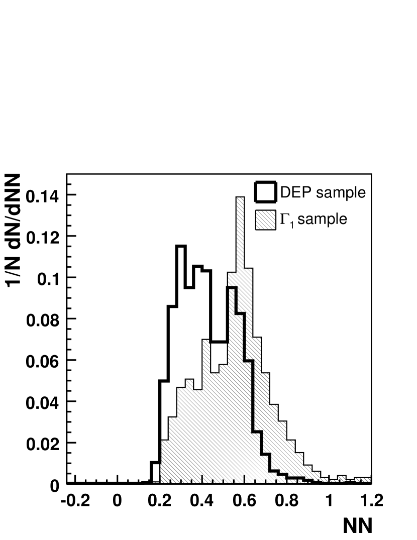
The three analysis methods are applied to the data samples defined in Section 2.2. The likelihood discriminant and neural network analysis are performed on the segment data samples (a) with information from the core electrode only and (b) with information from the core and the segment $S$ electrode. As an example, Figure 5 shows the output distributions for the two segment training data samples $DEP$ and $\Gamma_{1}$ for the likelihood method (left), the library method (middle) and the neural network (right). The segment pulse shapes have not been taken into account for these examples.

Figure 5: Output distributions for the two segment training data samples $DEP$ (open histograms) and $\Gamma_{1}$ (hatched histograms) for the likelihood method (left), the library method (middle) and the neural network (right). The segment pulse shapes were not taken into account in these examples.

The results of the analysis are interpreted in the following. First, it is shown that the electron-like and photon-like event samples can be distinguished. In a second step, the results are interpreted to distinguish between single-site and multi-site events. The estimate of the power of such a distinction requires the knowledge of the fraction of single-site and multi-site events in the data samples. That information is taken from the Monte Carlo simulation presented in Section 3 based on the parameter $R_{90}$.

5.1 Distinction between electron-like and photon-like event samples

The power to distinguish between electron-like and photon-like event samples is estimated. The events in the $DEP$ sample are assumed to give the same output in the analyses as events from neutrinoless double beta-decay. The cut values are chosen to keep 90% of the events in the $DEP$ training samples for the three analysis methods and thus a high detection efficiency. The fraction of events in each test data sample identified as electron-like are summarized in Table 3. The uncertainties are estimated from the deviation from 90% of the fraction of events identified as electron-like in the $DEP$ test data samples and found to be about 2%. Note that no deviation is found in case of the library method since the $DEP$ training data sample is used as a reference library.

Table 3: Fraction of events in the test data samples identified as electron-like for the three analyses. The uncertainties are estimated to be about 2%.

Data samples	$DEP$	$\Gamma_{1}$	$\Gamma_{2}$	$ROI$
	($1593$ keV)	($1620$ keV)	($2615$ keV)	(2039 keV)
Likelihood method
Core samples	89.3%	76.5%	75.4%	83.4%
Segm. samples, core only	89.3%	67.1%	64.1%	84.8%
Segm. samples, core & segm.	88.0%	66.7%	61.1%	83.4%
Library method
Core samples	90.0%	86.9%	85.8%	86.7%
Segm. samples, core only	90.0%	68.4%	56.4%	83.1%
Neural network method
Core samples	90.4%	65.8%	63.2%	79.9%
Segm. samples, core only	89.3%	54.1%	44.3%	80.8%
Segm. samples, core & segm.	89.3%	56.1%	49.9%	79.6%

The fraction of events identified as electron-like is significantly lower than 90% in the $\Gamma_{1}$, $\Gamma_{2}$ and $ROI$ samples. The fraction in the $\Gamma_{1}$ sample is found to be larger than that in the $\Gamma_{2}$ sample with each method. This is expected, as the mean free path of photons increases with the photon energy.

The fraction of events identified as electron-like in the $\Gamma_{1}$ and $\Gamma_{2}$ segment data samples (using the core pulse shape only) is found to be lower than that in the core data samples with all three methods. The additional usage of the segment pulse shape in the analyses reduces the fraction by maximally 3%; in case of the neural network it even increases the fraction by maximally 5%. This demonstrates that the additional information is highly correlated with the existing information and only marginally contributes to the analysis.

The neural network shows the best performance. This is expected, since the ANN uses the largest fraction of information and also takes correlations between input variables into account.

5.2 Selection of single-site events and discrimination against multi-site events

As demonstrated in Table 2, neither the $DEP$ nor the $\Gamma_{1}$, $\Gamma_{2}$ and $ROI$ samples are solely composed of single-site or multi-site events. The probability to correctly identify single-site and multi-site events as such, $\epsilon$ and $\eta$, can be deduced from the fraction of single-site and multi-site events in each sample (estimated from Monte Carlo) and the output of the analyses, $D$, $\chi^{2}_{\mathrm{min}}$, $NN$:

$$\epsilon = \frac{N_{id}^{SSE}/N_{true}^{MSE}-M_{id}^{SSE}/M_{true}^{MSE}}{N_{true}^{SSE}/N_{true}^{MSE}-M_{true}^{SSE}/M_{true}^{MSE}}\ ,$$ (7)

$$\eta = \frac{N_{id}^{MSE}/N_{true}^{SSE}-M_{id}^{MSE}/M_{true}^{SSE}}{N_{true}^{MSE}/N_{true}^{SSE}-M_{true}^{MSE}/M_{true}^{SSE}}\ ,$$ (8)

where $N_{id}^{SSE}$ and $N_{id}^{MSE}$ are the number of events in the $DEP$ sample identified as single-site and multi-site events, respectively. The numbers depend on the cut value chosen for each analysis. $N_{true}^{SSE}$ and $N_{true}^{MSE}$ are the true number of single-site and multi-site events in the same sample and are estimated from the Monte Carlo simulation discussed in Section 3. $M_{id}^{SSE}$ and $M_{id}^{MSE}$ are the number of events in the $\Gamma_{1}$ sample identified as single-site and multi-site events, respectively. $M_{true}^{SSE}$ and $M_{true}^{MSE}$ are the true number of single-site and multi-site events in the same sample. The probabilities $\epsilon$ and $\eta$ are assumed to be the same for all samples. This assumption is reasonable for the $DEP$ and $\Gamma_{1}$ samples as the average energies are very close.

The cut values for the three analysis methods are chosen to maximize the figure of merit, the identification efficiency $\sqrt{\epsilon\cdot\eta}$. Note, that these cut values differ from those used in Section 5.1. The probabilities obtained from the data samples using Equations 7 and 8 are listed in Table 4.

Table 4: Probabilities $\epsilon$ and $\eta$ obtained for all three analysis methods. The errors are introduced by the choice of $\overline{R}$ determining the fraction of single-site and multi-site events.

Analysis	$\epsilon$	$\eta$	$\sqrt{\epsilon\cdot\eta}$
Likelihood method
Core samples	($74.8^{+1.8}_{-0.3}$)%	($\phantom{0}84.7^{+\phantom{0}3.4}_{-\phantom{0}2.4}$)%	($79.6^{+1.4}_{-0.2}$)%
Segm. samples, core only	($84.3^{+1.8}_{-0.2}$)%	($\phantom{0}97.7^{+10.4}_{-\phantom{0}5.9}$)%	($90.8^{+4.8}_{-1.9}$)%
Segm. samples, core & segm.	($83.9^{+1.7}_{-0.1}$)%	($\phantom{0}94.0^{+\phantom{0}9.9}_{-\phantom{0}5.6}$)%	($88.8^{+4.6}_{-1.8}$)%
Library method
Core samples	($68.7^{+\phantom{0}0.8}_{-\phantom{0}0.1}$)%	($56.1^{+\phantom{0}1.4}_{-\phantom{0}1.0}$)%	($62.1^{+0.7}_{-0.2}$)%
Segm. samples, core only	($90.9^{+\phantom{0}0.1}_{-13.4}$)%	($80.4^{+10.1}_{-\phantom{0}9.1}$)%	($85.6^{+4.8}_{-1.7}$)%
Neural network method
Core samples	($85.6^{+2.4}_{-0.4}$)%	($\phantom{0}91.0^{+\phantom{0}4.3}_{-\phantom{0}0.3}$)%	($\phantom{0}88.3^{+1.9}_{-0.3}$)%
Segm. samples, core only	($96.4^{+2.5}_{-0.2}$)%	($121.6^{+15.0}_{-\phantom{0}8.5}$)%	($108.3^{+6.6}_{-2.5}$)%
Segm. samples, core & segm.	($90.6^{+2.3}_{-0.2}$)%	($115.4^{+13.4}_{-\phantom{0}7.7}$)%	($102.3^{+5.9}_{-2.2}$)%

The likelihood and library methods work better on events with only one segment hit. The additional usage of the segment pulse shape in the likelihood method does not improve the analysis results.

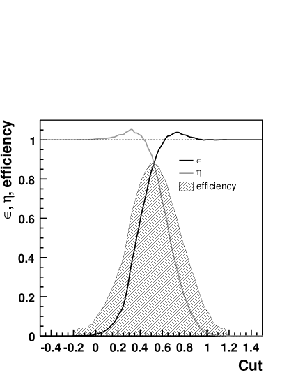
The analysis of the neural network output yields probabilities larger than one for the segment data samples. The calculation of $\epsilon$ and $\eta$ depends on the real fraction of single-site and multi-site events and is therefore model dependent. The current model assumes the fraction of single-site and multi-site events to be completely reflected by the parameter $R_{90}$. The validity of the assumed model is limited and the extraction of the probabilities $\epsilon$ and $\eta$ carries systematic uncertainties. The results should be taken with care. The efficiencies do not exceed unity for the chosen cut parameter for the core data samples. Figure 6 shows $\epsilon$ and $\eta$ together with the identification efficiency as a function of the neural network cut parameter for the core data samples.

Figure 6: Probabilities to correctly identify single-site, $\epsilon$, and multi-site events, $\eta$, and the efficiency, $\sqrt{\epsilon\cdot\eta}$, for the neural network analysis of the core data samples. Probabilities above one are caused by uncertainties in the extraction process.

5.3 Application to the ²²⁸Th data set

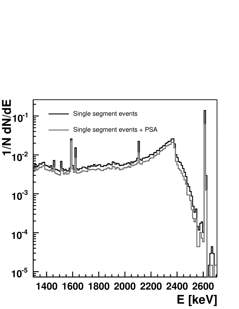
Figure 7 (left) shows the energy spectrum resulting from a ²²⁸Th source in the region from 1.3 MeV to 2.7 MeV as seen by the core electrode. The black line corresponds to all events with only segment $S$ hit, the gray line represents events with only segment $S$ hit and pulse shape analysis, using the ANN, applied. Only the pulse shape of the core was used and the cut parameter was chosen to keep 90% of the events in the $DEP$ training data sample.

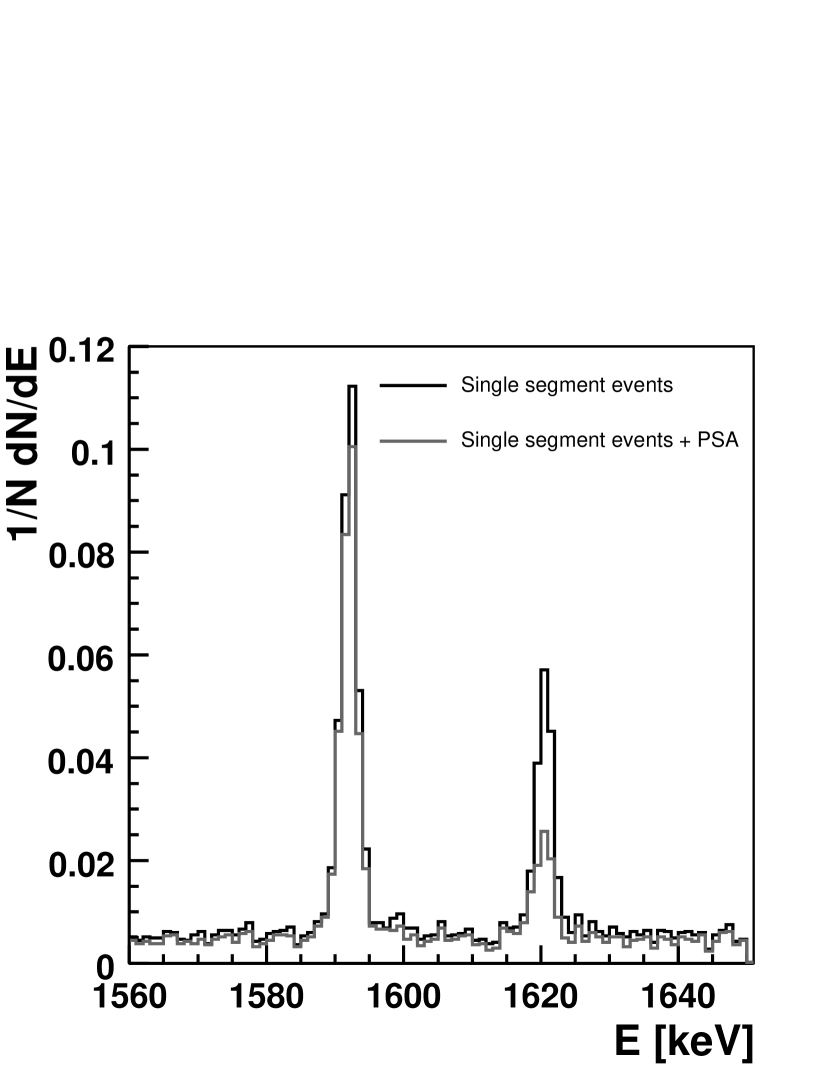
The gray spectrum is suppressed with respect to the black spectrum. The suppression ranges up to a factor of about two at the photon peaks. The suppression is weak in the double escape peak. Figure 7 (right) shows a close-up of the spectrum in the region from 1560 keV to 1650 keV. The application of the pulse shape analysis removes photon induced events (1620 keV photon line from the decay of ²¹²Bi) but keeps most of the electron induced events (double escape peak of the $2\ 615$ keV ²⁰⁸Tl photon at $1593$ keV). Pulse shape analysis is thus suitable to confirm the signal process.

Figure 7: Spectrum of a ²²⁸Th source as seen by the core electrode. The black line corresponds to all events with only segment $S$ hit, the gray line represents events with only segment $S$ hit and pulse shape analysis, using the ANN, applied. Only the pulse shape of the core was used and the cut parameter was chosen to keep 90% of the $DEP$ events. Left: Spectrum from 1.3 MeV to 2.7 MeV. Right: Close-up of the region from 1560 keV to 1650 keV. For a discussion see text.

6 Conclusions and outlook

Three methods using pulse shapes were introduced to distinguish electrons from multiply scattered photons. They were applied on data collected with a GERDA prototype detector. Single-site dominated samples were distinguished from multi-site dominated samples. The probability to correctly identify single-site and multi-site events was estimated based on Monte Carlo calculations.

All three methods were trained with double escape events and events from a nearby photon peak. The former events are expected to be similar to the expected $0\nu\beta\beta$-events.

The methods are based on information from the core electrode and may include information from the segment electrode or not. The power to identify photon induced events does not increase with the straightforward inclusion of the pulse shape of the segment.

The performance of the three methods is slightly worse than what was reported in [9]. A reason for this is the purity of the samples. Also, the spatial distribution of energy deposited inside the detector is not homogeneous in the $DEP$ sample. Methods to select cleaner and more homogeneous training samples are currently being tested.

The artificial neural network shows a better performance than both the likelihood discriminant and the library method. Photon peaks remaining after a single segment cut are suppressed by a factor of about two at energies around 1.5 MeV. At the same time 90% of the events in the single-site dominated sample are kept. This demonstrates that the association of a particular peak with the signal process can be substantiated by this kind of analysis.

The calculation of the efficiency to correctly identify single-site and multi-site events is limited by the assumed model based on the $R_{90}$ parameter. Further studies are required; in particular, a simulation of the development of pulse shapes is important and is currently under development. Studies using additional information from neighboring segments to distinguish single-site from multi-site events are also planned. In addition, an improved experimental setup is planned.

The rejection of events in the $1620$ keV peak using segment anti-coincidences as presented in [10] is about a factor of two better than the sole application of pulse shape analysis as presented in this paper. Nevertheless, the application of pulse shape analysis after a single segment cut can further reject events in this peak by an additional factor of about two.

7 Acknowledgements

The authors would like to thank A. Bettini, P. Grabmayr, L. Pandola and B. Schwingenheuer for their helpful comments and suggestions. The authors would also like to thank the GERDA and Majorana Monte Carlo groups for their fruitful collaboration and cooperation on the MaGe project.

References

- [1] S. Schönert et al. [GERDA Collaboration], Nucl. Phys. Proc. Suppl. 145 (2005) 242.
- [2] J. Simpson, J. Phys. G 31 (2005) S1801.
- [3] K. Vetter et al., Nucl. Instrum. Meth. A 452 (2000) 105.
- [4] J. Hellmig and H. V. Klapdor-Kleingrothaus, Nucl. Instrum. Meth. A 455 (2000) 638.
- [5] B. Majorovits and H. V. Klapdor-Kleingrothaus, Eur. Phys. J. A 6 (1999) 463 [arXiv:hep-ex/9911001].
- [6] D. Gonzalez et al., Nucl. Instrum. Meth. A 515 (2003) 634 [arXiv:hep-ex/0302018].
- [7] I. Abt et al. [GERDA Collaboration], Nucl. Instr. and Meth. A 570/3 (2007) 479.
- [8] C. E. Aalseth, Ph.D. Thesis, South Carolina U., UMI-30-06000.
- [9] S. R. Elliott, V. M. Gehman, K. Kazkaz, D. M. Mei and A. R. Young, Nucl. Instrum. Meth. A 558 (2006) 504, [arXiv:nucl-ex/0509026].
- [10] I. Abt et al., arXiv:nucl-ex/0701005.
- [11] I. Abt et al., arXiv:nucl-ex/0701004.
- [12] S. Agostinelli et al. [GEANT4 Collaboration], Nucl. Instrum. Meth. A 506 (2003) 250.
- [13] M. Bauer et al., Journal of Physics, Conf. Series. 39 (2006) 362.
-
[14]
C. G. Broyden, Journal of the Institute for Mathematics and Applications, 6, (1970) 222;
R. Fletcher, Computer Journal 13 (1970) 317;
D. Goldfarb, Mathematics of Computation 24 (1970) 23;
D. F. Shanno, Mathematics of Computation 24 (1970) 647;
See also summary in: D. F. Shanno, J. of Optimization Theory and Applications, 46, (1985) 87.