How tight is the Lieb-Oxford bound?

Abstract

Density-functional theory requires ever better exchange-correlation (xc) functionals for the ever more precise description of many-body effects on electronic structure. Universal constraints on the xc energy are important ingredients in the construction of improved functionals. Here we investigate one such universal property of xc functionals: the Lieb-Oxford lower bound on the exchange-correlation energy, $E_{xc}[n]\geq-C\int d^{3}r\,n^{4/3}$, where $C\leq C_{LO}=1.68$. To this end, we perform a survey of available exact or near-exact data on xc energies of atoms, ions, molecules, solids, and some model Hamiltonians (the electron liquid, Hooke’s atom and the Hubbard model). All physically realistic density distributions investigated are consistent with the tighter limit $C\leq 1$. For large classes of systems one can obtain class-specific (but not fully universal) similar bounds. The Lieb-Oxford bound with $C_{LO}=1.68$ is a key ingredient in the construction of modern xc functionals, and a substantial change in the prefactor $C$ will have consequences for the performance of these functionals.

I Introduction

Any numerical calculation of the electronic structure of matter that uses density-functional theory (DFT) employs an approximate exchange-correlation (xc) functional.kohnrmp ; dftbook ; parryang Further progress in DFT thus depends crucially on the development of ever better density functionals. A most important ingredient in this quest for better functionals is the small, but increasing, list of exact properties of and constraints on the universal xc functional.dftbook ; parryang ; perdewreview

In particular, this functional, $E_{xc}$, is known to satisfy the following inequalitiesperdewreview ; lp93

$$0\geq E_{xc}[n]\geq B[n]\geq-C\int d^{3}r\,n^{4/3},$$ (1)

where $C$ is a universal constant, $B[n]=\lim_{\gamma\to 0}\gamma^{-1}E_{xc}[n_{\gamma}]$, and $n_{\gamma}$ is the scaled density $n_{\gamma}({\bf r})=\gamma^{3}n(\gamma{\bf r})$. While the first inequality, providing an upper bound on $E_{xc}[n]$, is an immediate consequence of the variational principle, the second and third, providing lower bounds, are more complex. The second inequality, the Levy-Perdew bound,lp93 is based on scaling arguments. It contains $E_{xc}$ on the left and on the right, and thus provides a consistency test for any given approximation to $E_{xc}[n]$.

The third inequality is a remarkable result due to Lieb and Oxford,lopaper , who established the form of the bound and obtained the value $C_{LO}=1.68$ as an upper limitfootnote1 of the prefactor $C$. The present work is mostly concerned with this Lieb-Oxford bound, although a numerical comparison with the Levy-Perdew bound will also be given. In terms of the local-density approximation (LDA) to the exchange energy,

$$E_{x}^{LDA}[n]=-\frac{3}{4}\left(\frac{3}{\pi}\right)^{1/3}\int d^{3}r\,n^{4/3},$$ (2)

the LO bound can also be written asperdewreview ; lp93

$$E_{xc}[n]\geq\lambda_{LO}E^{LDA}_{x}[n],$$ (3)

where $\lambda_{LO}=1.354C_{LO}=2.275$. The analysis below is couched in terms of $\lambda$.

The Lieb-Oxford lower bound on the $xc$ energy is one of not many exactly known properties of the universal $xc$ functional. Similarly to other such properties, is has been used as a constraint in the construction of approximations to this functional.perdewreview It is satisfied, e.g., by the LDA,pw92 the PBE generalized-gradient approximationpbe (GGA) and the TPSS meta-GGA.tpss On the other hand, earlier GGAspw86 and semiempirical functionals containing fitting parametersb88 ; lyp are not guaranteed to satisfy the bound for all possible densities.

Note that Eq. (3) is a bound in the mathematical sense, i.e., $E_{xc}[n]$ can never be more negative than $\lambda_{LO}E^{LDA}_{x}[n]$. It is, however, not clear from the inequality itself if $\lambda_{LO}$ is the smallest possible value of the prefactor, i.e., if the bound can be tightened or not. Indeed, Chan and Handyhandylo have revisited the original calculation of Lieb and Oxford, and obtained the slightly tighter bound $\lambda_{CH}=2.2149$ (or $C_{CH}=1.6358$).

Independently of the question whether the bound can be tightened mathematically, it is not clear if nature actually makes use of the entire range of values of $E_{xc}$ allowed by the bound, and neither how distant specific classes of actual physical systems are from the mathematical maximum. To put these issues in clearer focus, note that for any actual density $n({\bf r})$ one can, in principle, evaluate the density functionals $E_{xc}$ and $E_{x}^{LDA}$ on this density, and calculate the ratio

$$\frac{E_{xc}[n]}{E_{x}^{LDA}[n]}=:\lambda[n],$$ (4)

which measures the weight of LDA exchange relative to the full exchange-correlation energy. The resulting value of $\lambda[n]$ must be smaller than or equal to $\lambda_{LO}=2.275$, for any $n$, but it is not a priori clear by how much, and neither what the variations of $\lambda$ over different classes of systems are.

Such information is not easy to obtain, since the definition (4) requires knowledge of the exact $xc$ energy in the numerator and of the exact density $n({\bf r})$ in the numerator and the denominator. This knowledge is, in general, not available. There are, however, certain classes of systems for which near-exact $xc$ energies and densities are available, e.g., from quantum Monte Carlo (QMC) or configuration interaction (CI) calculations. In this work we present a survey of avaliable such data for large and distinct classes of systems, and confront the results with the Lieb-Oxford bound.

Section II deals with real atoms, Sec. III with Hooke’s atom, Sec. IV with ions, Sec. V with a few molecules and Sec. VI with the homogeneous electron liquid. Sec. VII synthesizes the empirical analysis of Secs. II to VI in the form of two conjectures. Readers who do not want to go through the details of the analysis of different types of systems can go right to the conclusions, where all essential results are summarized.

Four appendices deal with issues that are loosely related to our main argument, or with by-products of our analysis that may be interesting in their own right. Appendix A motivates and presents a simple analytical fit to the atomic data analyzed in Sec. II. Appendix B contains a comparison of the Lieb-Oxford bound with the Levy-Perdew bound, appendix C classifies common (and some less common) parametrizations of the electron-liquid correlation energy with respect to the Lieb-Oxford bound, and appendix D discusses systems that violate the Lieb-Oxford bound.

II Lieb-Oxford bound in atoms

Table 1: Exchange-correlation energy, LDA exchange energy, and their ratio $\lambda$ for light atoms. First three rows (He, Be and Ne): Near-exact numerical $xc$ and $x$ energies from QMC data, evaluated on exact densities.umrigar ; burke Rows 4 to 20: Precise numerical $xc$ energies obtainedgoshparr from CI calculations and inversion of the KS equation by the ZMP procedure,zmp and exchange-only LDA energies obtained self-consistently on LDA-PW92 densities. For He, Be, and Ne these data are very similar to those obtained from QMC, illustrating that the resulting values of $\lambda$ are robust, and not contaminated with inaccuracies due to approximate densities.footnote2 All values are in atomic (Hartree) units.

	$-E_{xc}$	$-E_{x}^{LDA}$	$\lambda$
He	1.067	0.8830	1.208
Be	2.770	2.321	1.193
Ne	12.48	11.02	1.132
He	1.068	0.8617	1.239
Li	1.827	1.514	1.207
Be	2.772	2.290	1.210
B	3.870	3.247	1.192
C	5.210	4.430	1.176
N	6.780	5.857	1.158
O	8.430	7.300	1.155
F	10.320	8.999	1.147
Ne	12.490	10.967	1.139
Na	14.440	12.729	1.134
Mg	16.430	14.563	1.128
Al	18.530	16.486	1.124
Si	20.790	18.544	1.121
P	23.150	20.743	1.116
S	25.620	22.950	1.116
Cl	28.190	25.305	1.114
Ar	31.270	27.812	1.124

In order to calculate $\lambda[n]$ we need the exact LDA exchange energy, $E_{x}^{LDA}$, and the exact exchange-correlation energy $E_{xc}$, both on the exact density. For a few closed-shell atoms, near-exact $E_{xc}$ values and densities have been obtained by Umrigar and collaborators from QMC calculations.umrigar Of course, near-exact is not the same as mathematically exact, but the margin of error of these QMC data is much smaller than the effects we are after in this work.

The first three rows of Table 1 compare the near-exact $xc$ energies for He, Be and Ne (from Ref. umrigar, , as quoted in Ref. burke, ), the exact LDA exchange energies (obtained by evaluating the LDA functional for exchange on exact QMC densitiesumrigar ) and the resulting ratio $\lambda[n]=E_{xc}/E_{x}^{LDA}$. Two trends immediately leap to the eye: (i) the values of $\lambda$ are much smaller than the theoretical upper limit $\lambda_{LO}=2.275$, and (ii) $\lambda(Z)$ decreases as a function of atomic number $Z$.

To explore these emerging trends for a larger data set, the comparison is extended in the other rows of Table 1 to other atoms. For these atoms apparently no QMC results for $E_{xc}$ and the densities are available. The exchange-correlation energies reported in rows 4-20 were extracted from Ref. goshparr, , where they were obtained by numerical inversion of the Kohn-Sham (KS) equation on CI densities, following the Zhao-Morrison-Parr (ZMP) procedure.zmp The values for $E_{x}^{LDA}$ in rows 4-20 were calculated from the exact LDA exchange functional and evaluated at self-consistent LDA(PW92) densities.footnote2 For He, Be and Ne, the resulting values of $\lambda$ can be compared to those obtained from QMC. Cleary, both sets of data differ slightly, but this difference is a small fraction of the difference between the observed $\lambda$ values and the theoretical upper bound $\lambda_{LO}$. Additionally, we have employed approximate xc energies obtained from the B88-LYP GGA functional,b88 ; lyp which is highly precise for atoms (and, unlike similarly precise nonempirical functionals, such as PBE GGA and TPSS meta-GGA, does not make use of the Lieb-Oxford bound in its construction).

Figure 1 illustrates the simple and systematic trend of $\lambda$ as a function of $Z$, showing that the Lieb-Oxford bound with the originally proposed value $\lambda_{LO}=2.275$ is tightest for small $Z$, but actually rather generous for all atoms, typical values of $\lambda$ being about $50\%$ smaller. Note also that the QMC data, which are expected to be more precise than the CI-ZMP data, systematically predict still smaller values of $\lambda$. For the Ar atom ($Z=18$), and perhaps also the Be atom ($Z=4$), we suspect that the ZMP procedure has resulted in a less precise correlation energy than for the other atoms, because the correlation energy predicted for these atoms by the B88-LYP functional is much closer to the extrapolation of the QMC and other CI-ZMP data than their CI-ZMP values.

A simple fit to the B88-LYP data is

$$\lambda(Z)=0.993+\frac{0.313}{Z^{1/3}},$$ (5)

which is represented by the continuous line in Fig. 1. A physical motivation for the form of this fit is given in Appendix A.

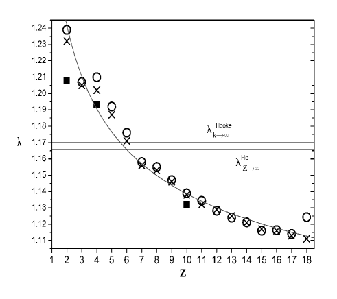
Figure 1: Value of the energy ratio $\lambda$, defined in Eq. (4) as a function of atomic number $Z$ for light atoms. Full squares: near-exact QMC data. Open circles: CI-ZMP data. Crosses: supplementary approximate data obtained from the B88-LYP functional. The upper limit $\lambda_{LO}$ is not shown in the figure, because on this scale it is too far from the actual values of $\lambda$. The two horizontal lines are estimates of $\lambda$ for Hooke’s atom and for the $Z\to\infty$ limit of Helium-like ions, discussed in Sec. III and Sec. IV. The continuous line represents the analytical expression (5), which is further discussed in Appendix A.

From Table 1 and Fig. 1 we conclude that for atoms $\lambda$ follows a simple and systematic trend as a function of $Z$, and always remains far from the upper limit $\lambda_{LO}=2.275$, approaching approximately half of this value as $Z\to 1$ and extrapolating to 1 as $Z\to\infty$. These conclusions are robust with respect to the various different ways of obtaining the densities and energies.footnote2 Additional comparisons with the Levy-Perdew bound [second inequality of Eq. (1)] are made in Appendix B.

III Lieb-Oxford bound in Hooke’s atom

Table 2: Exact exchange-correlation and LDA exchange energies of Hooke’s atom, evaluated on the exact densities, for different values of the spring constant $k$. Data for $k=0.25$ and $k=3.6\times 10^{-6}$ (row one and two) are from Ref. FiliUmTaut, . Alternative data for $k=0.25$ (row three) are from Ref. kais, , and the $k\to\infty$ limit has been extracted in the way described in the main text, from data in Ref. laufer, .

k	$E_{xc}$	$E_{x}^{LDA}$	$\lambda$
$3.6\times 10^{-6}$	-0.0259	-0.0174	1.49
0.25	-0.5536	-0.4410	1.255
0.25	-0.555	-0.4410	1.26
$k\rightarrow\infty$			1.17

Hooke’s atom is a model system in which two electrons interact via Coulomb’s law but are bound to a harmonic potential instead of a $1/r$ potential. It is frequently used in discussing approximate $xc$ functionals and other aspects of DFT, and many exact and numerical results for it are known.kestner ; laufer ; gill ; kais ; ivanov ; taut ; trickey

The Hamiltonian of Hooke’s atom is

$$\hat{H}_{\rm Hooke}(k)=-\frac{\hbar^{2}}{2m}(\nabla_{1}^{2}+\nabla_{2}^{2})+{1\over 2}k(r_{1}^{2}+r_{2}^{2})+\frac{e^{2}}{|{\bf r}_{1}-{\bf r}_{2}|}.$$ (6)

It describes two interacting electrons confined in space by a harmonic potential of strength $k$. Since the two electrons in this atom interact by the same Coulomb interaction $1/r_{12}$ as in real atoms, this system has the same $xc$ functional. The replacement of the nuclear potential by a harmonic confinement, on the other hand, greatly simplifies the solution of the eigenvalue problem posed by Eq. (6) This fact has motivated much work on this simple, yet nontrivial, model.kestner ; laufer ; gill ; kais ; ivanov ; taut ; trickey

For the present purposes we are interested in the ratio $\lambda[n]$, which we rewrite as

$$\lambda[n]=\frac{E_{x}[n]}{E_{x}^{LDA}[n]}+\frac{E_{c}[n]}{E_{x}^{LDA}[n]}.$$ (7)

Laufer and Kriegerlaufer have shown that for $k\to\infty$ the LDA exchange energy evaluated on the exact density recovers $85.5\%$ of the exact exchange energy of Hooke’s atom. Hence, for large $k$ (high curvature),

$$\frac{E_{x}^{LDA}}{E_{x}}=0.855.$$ (8)

As $k\to\infty$, the correlation energy of Hooke’s atom rapidly drops to zero, relative to the exchange energy. Hence, we can neglect the second term in Eq. (7) and estimate $\lambda^{Hooke}$ from the inverse of Eq. (8), which yields

$$\lambda^{Hooke}_{k\to\infty}=1.17,$$ (9)

The value $\lambda_{k\to\infty}^{Hooke}$ is shown as a horizontal line in Fig. 1.

Exact data at some finite values of $k$, including correlation, have been presented in Refs. kais, and FiliUmTaut, . These data are collected in Table 2. The two independent calculations for $k=0.25$ are in excellent agreement, and the tendency as a function of $k$ is consistent with our estimate of the $k\to\infty$ limit. Clearly, $\lambda$ for Hooke’s atom is very close to its value for real atoms, and far below the limiting value $\lambda_{LO}$.

IV Lieb-Oxford bound in ions from the Helium isoelectronic series

Near-exact numerical data for some representatives of the Helium isoelectronic series have been obtained from Hylleraas wave functions by Umrigar and Gonze,umrgonze and are displayed in Table 3. Laufer and Kriegerlaufer also consider the large $Z$ limit of the Helium isoelectronic series, for which they find $E_{x}^{LDA}/E_{x}=0.8577$. From this we obtain, by the same reasoning used for Hooke’s atom,

$$\lambda^{He}_{Z\to\infty}\approx 1.166.$$ (10)

The value $\lambda^{He}_{Z\to\infty}$ is shown as a horizontal line in Fig. 1, and also included in Table 3.

The trend of the data in Table 3 as a function of $Z$ is indeed consistent with $\lambda^{He}_{Z\to\infty}\approx 1.166$. Interestingly, the value of $\lambda$ for the He isoelectronic series is very similar to that of Hooke’s atom, in particular in the limit of very strongly confining external potentials ($Z\to\infty$ and $k\to\infty$, respectively). For all values of $Z$, including negative and positive ions, the resulting values of $\lambda$ are much smaller than $\lambda_{LO}$.

Table 3: Near-exact exchange-correlation energies and LDA exchange energies of ions, evaluated on the exact densities, from Ref. umrgonze, , and the resulting value of $\lambda$. The $Z\to\infty$ limit is that of Eq. (10). All energies are in Hartree units.

Z	$E_{xc}$	$E_{x}^{LDA}$	$\lambda$
1 (H-)	-0.422893	-0.337	1.25
4 (Be2+)	-2.320902	-1.957	1.186
10(Ne8+)	-6.073176	-5.173	1.174
80(Hg78+)	-49.824467	-42.699	1.1669
$Z\to\infty$			1.166

V Lieb-Oxford bound in molecules

Exchange-correlation energies for the silicon dimer and a few small hydrocarbons have been obtained by Variational Monte Carlo (VMC) techniques by Hsing et al.hsing These data, together with the resulting values of $\lambda$, are recorded in Table 4.

Table 4: VMC exchange-correlation energies and LDA exchange energies of a few small molecules,hsing and the resulting values of $\lambda$. Last row: DMC data for bulk Si, from Ref. cancio, .

molecule	$E_{xc}$	$E_{x}^{LDA}$	$\lambda$
C2H2	-3.840	-3.428	1.120
C2H4	-4.606	-4.110	1.121
C2H6	-5.367	-4.760	1.128
Si2	-2.028	-1.762	1.151
Si(bulk)	-33.23	-27.66	1.201

The resulting values of $\lambda$ are quite similar to those obtained for atoms. Interestingly, $\lambda$ of the hydrocarbons is smaller than that of the C atom, whereas $\lambda$ of the silicon dimer is a bit larger than that of the Si atom. Also, $\lambda$ for the hydrocarbons slowly grows as a function of the number of H atoms. If there is any trend as a function of electron number, it is very weak, as is demonstrated by the bulk limit, for which included in the Table the DMC value for bulk Si, from Ref. cancio, .

Unfortunately, this data set may be too small to draw any reliable inferences from such trends. What is beyond doubt, however, is that the molecular data predict $\lambda$ values that are roughly as far away from the limit $\lambda_{LO}$ as previously found for atoms and ions.

VI Lieb-Oxford bound in the electron liquid

The calculations of the previous sections show that for localized atomic, ionic and molecular densities the Lieb-Oxford bound is rather generous. The strength of the original Lieb-Oxford argument, however, rests in the fact that is holds for arbitrary densities, and not just for certain subsets. In order to extend the investigation to a completely different class of densities we thus now turn to spatially uniform systems. A priori there is no reason why one would expect similar values of $\lambda[n]$ to the ones found for localized density distributions, although the value for bulk Si, mentioned at the end of the previous section, strongly suggests so.

The homogeneous electron liquid is, of course, of paramount importance for DFT, as the reference system on which the construction of the LDA and many GGAs and meta-GGAs are based. It is also of interest in its own right as a model for the conduction band of simple metals and as a many-body system in which effects of the particle-particle interaction can be studied without the simultaneous presence of complications due to inhomogeneity in the single-body potential.quantliq

The per-particle exchange energy of the homogeneous electron liquid is

$$e_{x}(r_{s})=-\frac{3}{4\pi}\left(\frac{9\pi}{4}\right)^{1/3}\frac{1}{r_{s}}=:-\frac{D_{0}}{r_{s}},$$ (11)

where $r_{s}$ is the usual electron-liquid parameter related to the charge density $n$ via $r_{s}=(4\pi n/3)^{-1/3}$. Below we adopt the value $D_{0}=0.4581653$, but note that the constants in the various parametrizations considered below are not normally known to this number of significant digits. For the electron liquid, and only for the electron liquid, the LDA is by construction exact, and Eq. (4) becomes

$$\lambda(r_{s})=\frac{e_{x}(r_{s})+e_{c}(r_{s})}{e_{x}(r_{s})}=1+\frac{e_{c}(r_{s})}{e_{x}(r_{s})}.$$ (12)

The per-particle correlation energy of the electron liquid is not known in closed form, but the PW92 parametrization,pw92 ; primer

$$e_{c}(r_{s})=-2c_{0}(1+\alpha_{1}r_{s})\times$$

$$\ln\left[1+\frac{1}{2c_{0}(\beta_{1}r_{s}^{1/2}+\beta_{2}r_{s}+\beta_{3}r_{s}^{3/2}+\beta_{4}r_{s}^{2})}\right]$$ (13)

is the best available fit to the Green’s function Monte Carlo data of Ref. ceperley, . In Eq. (13) $c_{0}=0.031091$, $\beta_{1}=7.5956$, $\beta_{2}=3.5875$, $\beta_{3}=1.6382$, $\beta_{4}=0.49294$ and $\alpha_{1}=0.21370$ are determined such as to reproduce the exactly known properties and the QMC data for $e_{c}(r_{s})$.pw92 ; primer

The unique combination of facts that the LDA becomes exact for the electron liquid and that $e_{c}$ is known to very high precision, allows us to study $\lambda$ as a continuous function of the density parameter $r_{s}$, instead of at isolated densities, as in the previous sections.

The high-density limit is, rigorously, $\lambda(r_{s}\to 0)=1$, because $\lim_{r_{s}\to 0}e_{c}(r_{s})/e_{x}(r_{s})=0$. To determine the low-density limit, recall the leading term of the large-$r_{s}$ expansion of the correlation energy,pw92

$$e_{c}(r_{s}\to\infty)=-\frac{d_{0}}{r_{s}}+\ldots,$$ (14)

where, according to best estimates pw92 , $d_{0}=0.43776$. This gives the electron-liquid limit for $\lambda$,

$$\lambda(r_{s}\to\infty)=1+\frac{-d_{0}/r_{s}}{-D_{0}/r_{s}}=1.9555.$$ (15)

This limit is only of formal relevance, as at $r_{s}\approx 65\pm 10$ the electron liquid becomes unstable with respect to the Wigner crystal,ballone and the homogeneous phase ceases to be the ground state. Thus, the largest physically possible value of the uniform electron liquid is $\lambda(r_{s}\approx 65)=1.65$. (This value changes only very little, if the older and presumably less accurate estimateceperley $r_{s}=100\pm 20$ for the liquid-to-crystal transition is used instead.)

The quantity $d_{0}$ can also be evaluated by employing in Eq. (12) available parametrizations of the electron-liquid correlation energy. From the PW92 parametrization, as specified above, one finds, for example,

$$\lambda^{PW92}(r_{s}\to\infty)=1+\frac{\alpha_{1}}{\beta_{4}}\frac{4\pi}{3}\left(\frac{4}{9\pi}\right)^{1/3}=1.9462.$$ (16)

A classification of common (and some less common) parametrizations of the electron-liquid correlation energy with respect to the Lieb-Oxford bound is presented in Appendix C.

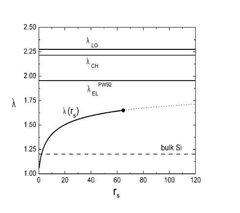
Figure 2: Value of the ratio $\lambda$, defined in Eq. (4), as a function of the density parameter $r_{s}$ of the homogeneous electron liquid, using the PW92 parametrization (13) for the correlation energy. The four horizontal lines correspond, from top to bottom, to the Lieb-Oxfordlopaper value $\lambda_{LO}$, the Chan-Handyhandylo value $\lambda_{CH}$, the low-density limit $\lambda_{r_{s}\to\infty}^{PW92}$, and the value for bulk $Si$, from Table 4. Note that actual metals are located at the very left margin of the plot, which we have extended to unphysically large $r_{s}$ values only to display the large remaining distance to $\lambda_{LO}$. The filled circle indicates the $r_{s}$ value where the transition to the Wigner crystal is expected to occur,ballone and the uniform electron liquid ceases to be the ground state.

We note that the best estimate of $d_{0}$ still yields a value of $\lambda(r_{s}\to\infty)$ that is substantially smaller than the value $\lambda_{LO}$. Since the value $\lambda(r_{s}\to\infty)$ is itself an upper limit of $\lambda(r_{s})$ at all densities of the electron liquid, this implies that in the entire range from $r_{s}=0$ to $1/r_{s}=0$ the Lieb-Oxford bound can be substantially tightened.

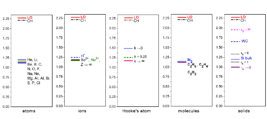
Figure 3: Graphical summary of all investigated systems. Each panel shows, on the same scale, the Lieb-Oxford bound and its refinement by Chan and Handy, together with actual values of $\lambda$ obtained from QMC or CI calculations, or exactly. The first panel shows that the entire periodic table fits in a small stretch of $\lambda$ values bounded from above by that of the $He$ atom. Ions, small molecules, Hooke’s atom, and solids – represented by bulk Si and the electron liquid – occupy almost the same region of $\lambda$ space. Values above $\lambda=1.35$ are found only for unphysical limits of model Hamiltonians ($r_{s}\to\infty$ of the electron liquid, or $k\to 0$ of Hooke’s atom).

This is illustrated in figure 2, which shows a plot of $\lambda(r_{s})$ resulting from the PW92 parametrization over a wide density interval. Clearly, $\lambda(r_{s})$ interpolates smoothly between the known limits, and remains far from its theoretical upper limit $\lambda_{LO}$ for any density. Figure 2 and the value $\lambda({r_{s}\to\infty})=1.9555$ show that for any possible density of the electron liquid the Lieb-Oxford bound falls way above the actual value of $\lambda$. For metallic densities, $r_{s}\approx(2\ldots 6)$, $\lambda$ is even smaller, not passing $1.333$.

The $\lambda$ value of bulk Si, $\lambda=1.201$, included in Table 4, falls near the center of the $\lambda$ interval obtained for the electron liquid in the metallic density range, although bulk Si is not a metal. This again indicates that the shape of the density distribution is fairly unimportant for the value of $\lambda$, which never seems to come even near the maximum $\lambda_{LO}=2.275$.

VII Conclusions

The two quantities, $\lambda[n]$ and $\lambda_{LO}$, considered in this paper have different meanings. $\lambda[n]$, as defined in Eq. (4), measures the (inverse) weight of LDA exchange in the full exchange-correlation energy of an actual physical system, or a model of a physical system. We found here that across very different types of systems $\lambda[n]$ does vary, but not very strongly. $\lambda_{LO}$, as defined in Eq. (3), is a mathematical upper limit to $\lambda[n]$, which is the same for all nonrelativistic three-dimensional systems with Coulomb interactions.

The analysis of these two quantities, performed in the preceding sections, can be summarized as follows: The Lieb-Oxford bound provides a lower bound on the $xc$ energy of any (nonrelativistic three-dimensional Coulomb) system, but nature does not necessarily make use of the entire range of permitted values, up to $\lambda_{LO}=2.275$. Neutral atoms have $\lambda$ near $1$ and approach $1$ more closely as the atomic number $Z$ is increased. In this limit LDA exchange thus captures a larger part of the full $xc$ energy. Positive and negative ions, Hooke’s atom, small molecules and bulk Si all have $\lambda$ values that are close to those of isolated atoms, and far from $\lambda_{LO}$. The electron liquid at metallic densities has $\lambda$ close to $1.3$, approaching $1$ and $1.65$ in the extreme high and low-density limits, respectively.

Figure 3 contains a graphical summary of our analysis. Fine details are not visible on the scale of the figure, but the overall impression is very clear, and strongly suggests that the LO bound is too generous. A tendency that systems with a more dilute and spread-out density distribution produce larger $\lambda$ values is clearly visible for Hooke’s atom and the electron liquid. For atoms and ions, we find that lighter systems produce larger $\lambda$ values. For all investigated systems, $\lambda$ is much smaller than $\lambda_{LO}=2.275$. Situations leading to the, relatively, largest $\lambda$ values can be classified as follows:

(i) The largest values of $\lambda$ we found in this investigation arise in unphysical low-density limits of model Hamiltonians (the $k\to 0$ limit of Hooke’s atom, or the $r_{s}\to\infty$ limit of the electron liquid). The largest value we have found including such limits is $\lambda_{max}=1.9555$, for the unattainable low-density limit of the electron liquid.

(ii) If we exclude physically unrealizable limits of a parameter approaching infinity or zero, the largest value we have found for physically possible parameters is $\lambda_{max}=1.65$, for the very low-density uniform electron liquid, right at its transition to the Wigner crystal.

(iii) The largest value we have found for any actual physical system (atoms, ions, molecules, and solids, but excluding Hooke’s atom and the electron liquid, which are idealized models) is $\lambda_{max}=1.25$, for the H^- ion.

This sequence of observations suggests two conjectures.

Strong conjecture: Tightening the bound for all densities. The Lieb-Oxford bound can be substantially tightened, in the mathematical sense. Independent support for this conjecture comes from recent numerical work of Chan and Handy,handylo who indeed found that $\lambda_{LO}$ can be replaced by the slightly smaller value $\lambda_{CH}=2.2149$. The present investigation suggests, however, that a much larger reduction may be achievable.

It is, of course, conceivable that for certain special densities $\lambda[n]$ comes arbitrarily close to $\lambda_{LO}$ (or $\lambda_{CH}$), but if this is not the case for systems as different as uniform electron liquids and isolated atoms and ions, and moreover, if the distance from the actual $\lambda$ in these systems to $\lambda_{LO}$ is a large fraction of $\lambda_{LO}$ itself, it becomes a very real possibility that $\lambda_{LO}$ is not the tightest possible limit. Still, if it should turn out to be possible to construct (perhaps pathological) density distributions that require keeping the upper limit at $\lambda=\lambda_{LO}$ (or $\lambda_{CH}$), this would still be compatible with the following weaker conjecture.

Weak conjecture: Tightening the bound for physical densities. For physical densities (arising from realistic Hamiltonians, excluding unphysical limits) the Lieb-Oxford bound can be substantially tightened. In fact, our collection of data on different systems suggests a limit of $\lambda_{conjec}\approx 1.35$, instead of $\lambda_{LO}=2.275$. Interestingly, and somewhat suggestively, this empirically found value of $\lambda$ makes the prefactor $C$ in $E_{xc}[n]\geq-C\int d^{3}r\,n^{4/3}$ equal to unity.

Many existing density functionals, such as the PBE GGA pbe and the TPSS meta-GGA tpss employ the Lieb-Oxford bound, with $\lambda_{LO}=2.275$, as a constraint in their construction. It should be most interesting to explore if a change of $\lambda$ to a somewhat lower value, either universally or for classes of systems, has an impact on the performance of these functionals in applications in electronic-structure calculations.

Acknowledgments This work was supported by FAPESP and CNPq. Useful conversations with Irene D’Amico and H. J. P. Freire are gratefully acknowledged.

Appendix A Fit to the atomic data

The systematic trend displayed by the atomic data in Fig. 1 suggests that their behaviour follows a simple law as a function of $Z$. A reasonable form for this law can be guessed as follows: The correct value of $\lambda(Z\to\infty)$ is probably exactly one, because asymptotically exchange dominates correlation, and LDA exchange becomes exact.pcsb For finite $Z$, we recall that in generalized Thomas-Fermi theoryspruch all energy contributions are expanded powers of $Z^{1/3}$, so that the energy ratio $\lambda$ should also involve such powers. Since $\lambda(Z)$ decreases with increasing $Z$, the simplest expression consistent with these expectations is

$$\lambda(Z)=A_{1}+\frac{A_{2}}{Z^{1/3}},$$ (17)

where $A_{2}$ is a prefactor that cannot be determined by such generic considerations, and we allow $A_{1}$ to deviate slightly from unity, because the available data points are not exact.

A simple fit of this expression to the data in Fig. 1 predicts $A_{1}=1.03$ and $A_{2}=0.231$ if only the three QMC data points are considered, $A_{1}=0.986$ and $A_{2}=0.331$ for the CI-ZMP data (except Ar, which, as explained above, may not be properly represented by the CI-ZMP data), and $A_{1}=0.993$ and $A_{2}=0.313$ for the approximate B88-LYP data, up to $Ar$. Reasuringly, the fitted values of $A_{1}$ are close to the theoretical expectation $A_{1}=1$. The third of these fits is shown as continuous curve in Fig. 1.

This simple fit already accounts well for the data in Fig. 1, suggesting that the proposed $Z^{-1/3}$ behaviour is quite realistic. Better fits could, of course, be obtained by allowing more terms in the fitting function. However, our aim here is not to obtain the best possible fit to the data points but to illustrate that for atoms the prefactor $\lambda$ has a simple and systematic trend as a function of $Z$.

Appendix B Levy-Perdew bound in atoms

Table 5: Comparison of the Levy-Perdew bound and the Lieb-Oxford bound. Values of $B$ are taken from Ref. lp93, , where they are obtained from a modified PW91 functional, evaluated at Hartree-Fock densities. The values for $\lambda$ of He and Ne are QMC data from Table 1. For Ar and Kr, Ref. lp93, also provides values for $B$, but for Kr there do not seem to exist QMC or CI-ZMP data, and for Ar the CI-ZMP value is so far off the curve describing the other atoms (see Fig. 1) that we do not trust it. Hence, we evaluated $\lambda$ for Ar and Kr selfconsistently from the B88-LYP functional, which is highly precise for atoms. To illustrate the error that arises from using an approximate functional, we have also included, in row 3, the value of $\lambda$ predicted by the B88-LYP functional for Ne.

	$\lambda$	$B/E_{x}^{LDA}$
He	1.208	1.900
Ne	1.132	1.920
Ne	1.138
Ar	1.111	1.926
Kr	1.079	1.931

For the He, Ne, Ar and Kr atoms we can compare the Lieb-Oxford to the Levy-Perdew bound [second inequality of Eq. (1)]. Our analysis is based on the data in Table 1 of Ref. lp93, , which reports values of the quantity $B[n]=\lim_{\gamma\to 0}\gamma^{-1}E_{xc}[n_{\gamma}]$ for one of the best available GGAs (which at the time of writing of Ref. lp93, was a slightly modified PW91pw91 ), evaluated on tabulated Hartree-Fock densities. To the extent that the PW91 functional and the tabulated Hartree-Fock densities can be trusted as approximations to the exact ones, the quantity $B^{PW91}[n^{HF}]$ should, according to Eq. (1), provide a tighter bound on $E_{xc}$ than the Lieb-Oxford inequality, as indeed it was found to do.lp93

The corresponding values of the ratio $B^{PW91}[n^{HF}]/E_{x}^{LDA}[n^{HF}]$ should thus be smaller than $\lambda_{LO}$ but still larger than the actual ratio $\lambda$, defined in our Eq. (4), thus leading to the chain of inequalities

$$\frac{E_{xc}}{E_{x}^{LDA}}=\lambda\leq\frac{B}{E_{x}^{LDA}}\leq\lambda_{LO}.$$ (18)

The data in Table 5 show that this expectation is bourne out, and that even the Levy-Perdew bound is still considerably above the actual (near exact) value of $\lambda$. Interestingly, the tendencies of $\lambda$ and of $B/E_{x}^{LDA}$ as functions of $Z$ are opposite, the former decreasing and the latter increasing.

Appendix C Electron-gas correlation energy

We recall from Sec. VI that the electron liquid displays the largest values of $\lambda$ in the low-density limit, $r_{s}\to\infty$, where

$$\lambda=1+\frac{e_{c}}{e_{x}}\to 1+\frac{d_{0}}{\frac{3}{4\pi}\left(\frac{9\pi}{4}\right)^{1/3}}=1.9555.$$ (19)

Many interpolations and parametrizations of $e_{c}(r_{s})$ have been proposed over the years. In Table 6 we list the values of $d_{0}$ and $\lambda(r_{s}\to\infty)$ predicted by Wigner’s original interpolation formula (W),wigner the modification of Wigner’s expression by Brual and Rothstein (BR);BrualR the parametrizations of Gunnarsson and Lundqvist (GL)GunnarsonL and von Barth and Hedin (vBH),vBH which are based on perturbation theory; those of Vosko, Wilk and Nusair (VWN),VWN Perdew and Zunger (PZ81),PZ81 and Perdew and Wang (PW92),pw92 based on Monte Carlo data; a simple electrostatic estimate presented in Ref. primer, , and the recent proposal by Endo et al. (EHTY),ehty which was specifically designed for the $r_{s}\to 0$ limit.

Table 6: Coefficient $d_{0}$ and ratio $\lambda$ for common, and some less common, parametrizations of the electron-liquid correlation energy.

Funcional	$d_{0}$	$\lambda(r_{s}\to\infty)$
W	0.44000	1.9604
BR	0.02890	1.0631
GL	0.28472	1.6214
vBH	0.56700	2.2375
VWN	0.41433	1.9043
PZ81	0.42681	1.9316
PW92	0.43352	1.9462
EHTY	1.1189	$\infty$
elstat.est.	0.90000	2.9644
near-exact	0.43776	1.9555

The entries in Table 6 fall in three classes. First, the electrostatic estimate and the EHTY parametrization violate the Lieb-Oxford bound even in its most generous universal form, employing $\lambda_{LO}$. This is not a surprise, considering the crudeness of the electrostatic estimate and the fact that the EHTY parametrization was designed to work well in the $r_{s}\to 0$ limit, not the $r_{s}\to\infty$ limit. Second, the von Barth-Hedin parametrization and Wigner’s interpolation formula obey the Lieb-Oxford bound in its universal form, but violate the stricter electron-liquid limit, which a proper LDA must also obey. Third, all other functionals are consistent also with this stricter limit. We do not recommend the use of any xc functional from the first or second class. The BR functional, which was fitted to data on the He atomBrualR is a special case, as it predicts a value of $d_{0}$ that obeys all bounds, but is way off the best available value. Hence, we do not recommend the use of this expression for extended systems.

Appendix D Systems violating the Lieb-Oxford bound

Elsewhere in this paper we have repeatedly refered to the Lieb-Oxford bound as universal. This use of the concept of universality is the same commonly employed in DFT: a universal quantity (such as the Hohenberg-Kohn functional $F_{HK}$) or property (such as the Lieb-Oxford bound) is one that is the same for all systems that share common kinetic-energy and interaction-energy operators. In particular, such quantities or relations are independent of the external potentials. Since the Lieb-Oxford bound is universal in this sense, we could confront it, above, with data on a wide variety of different systems.

The kinetic-energy operator changes, e.g, in relativistic quantum mechanics. Even in nonrelativistic quantum mechanics it changes if the dimensionality is reduced. We stress that the Lieb-Oxford bound was derived for nonrelativistic three-dimensional systems,lopaper and it is not clear if similar results hold in two or one dimensions, or relativistically. If similar bounds can be shown to hold, we expect that the prefactor $\lambda_{LO}$ (or $C_{LO}$) will be different.

The interaction-energy operator changes, e.g., when DFT is applied to model Hamiltonians.baldalett ; confined ; hemoprb ; magyar An interesting example is the Hubbard model, where the interaction is local (acting only between electrons at the same site) and spin-selective (acting only between electrons of opposite spins).

For fermions, the wave function of the Hubbard model is properly antisymmetrized, but this has no consequences for the energy, i.e., the exchange energy is rigorously zero. The local-density approximation for the Hubbard model, constructed in Ref. baldalett, and applied, e.g., in Refs. mottlett, ; superlattice, ; coldatoms, , respects this property. Hence, the Lieb-Oxford bound in its Coulomb-interaction form

$$E_{xc}[n]\geq\lambda_{LO}E^{LDA}_{x}[n]$$ (20)

cannot hold for the Hubbard model, because the right-hand side is rigorously zero, whereas the left-hand side is known to be nonzero and negative. Similar conclusions hold for other model Hamiltonians whose interaction is not of Coulomb form.

References

- (1) W. Kohn, Rev. Mod. Phys. 71, 1253 (1999).
- (2) R. M. Dreizler and E. K. U. Gross, Density Functional Theory (Springer, Berlin, 1990).
- (3) R. G. Parr and W. Yang, Density-Functional Theory of Atoms and Molecules (Oxford University Press, Oxford, 1989).
- (4) J. P. Perdew, A. Ruzsinszky, J. Tao, V. N. Staroverov, G. E. Scuseria and G. I. Csonka, J. Chem. Phys. 123, 062201 (2005).
- (5) M. Levy and J. P. Perdew, Phys. Rev. A 48, 11638 (1993).
- (6) E. H. Lieb and S. Oxford, Int. J. Quantum Chem. 19, 427 (1981).
- (7) A lower bound on is also known,lopaper but not immediately useful for the construction of approximate functionals: to obtain a true lower bound on the (negative) functional one requires an upper bound for the (positive) quantity . We therefore focus in this paper on this upper bound, , which is the value used as input in the construction of nonempirical functionals.
- (8) J. P. Perdew and Y. Wang, Phys. Rev. B 45, 13244 (1992).
- (9) J. P. Perdew, K. Burke and M. Ernzerhof, Phys. Rev. Lett. 77, 3865 (1996).
- (10) J. Tao, J. P. Perdew, V. N. Staroverov and G. E. Scuseria, Phys. Rev. Lett. 91, 146401 (2003); J. Chem. Phys. 119, 12129 (2003); J. Chem. Phys. 120, 6898 (2004); Phys. Rev. B 69, 075102 (2004).
- (11) J. P. Perdew and Y. Wang, Phys. Rev. B 33, 8800 (1986). J. P. Perdew, Phys. Rev. B 33, 8822 (1986).
- (12) A. D. Becke, Phys. Rev. A 38, 3098 (1988).
- (13) C. Lee, W. Yang and R. G. Parr, Phys. Rev. B 37, 785 (1988).
- (14) G. K.-L. Chan and N. C. Handy, Phys. Rev. A 59, 3075 (1999).
- (15) C. J. Umrigar and X. Gonze, in High Performance Computing and its Application to the Physical Sciences, Proceedings of the Mardi Gras 1993 Conference, eds. D. A. Browne et al. (World Scientific, Singapore, 1993). C. Filippi, X. Gonze and C. J. Umrigar, in Recent Developments and Applications of Modern Density Functional Theory, ed. J. Seminario (Elsevier, Amsterdam, 1996).
- (16) F. G. Cruz, K.-C. Lam and K. Burke, J. Phys. Chem. A 102, 4911 (1998).
- (17) R. G. Parr and S. K. Ghosh, Phys. Rev. A 51, 3564 (1995).
- (18) Q. Zhao, R. C. Morrison and R. G. Parr, Phys. Rev. A 50, 2138 (1994).
- (19) To make sure that our conclusions are stable with respect to changes in the employed parametrizations and numerical procedures, the ratio for neutral atoms was also evaluated in a variety of other ways. These include (i) obtaining the exact energies not from QMC or ZMP-CI, but by subtracting the result of a self-consistent Hartree calculation from total energies obtained by full CI,froese (ii) using also for He, Be and Ne approximate energies and densities, obtained from the B88-LYPb88 ; lyp functional, instead of the exact ones, (iii) employing the PZ81 and (iv) the VWN parametrizations in the self-consistent LDA calculation of the exchange energies and densities, instead of PW92, (v) employing no parametrization of at all, i.e., obtaining the exchange energy on exchange-only densities, and (vi) using VMC and DMC correlation energies from Ref. drummond, instead of those from CI. (Note that the correlation energies of Refs. froese, and drummond, are defined with respect to Hartree-Fock exchange, not Kohn-Sham exchange, and thus slightly different from Kohn-Sham correlation energies.) All these changes in the procedure lead only to changes in the final results that are much smaller than the difference between the resulting values of and the Lieb-Oxford limiting value .
- (20) N. R. Kestner and O. Sinanoglu, Phys. Rev. 128, 2687 (1962).
- (21) P. M. Laufer and J. B. Krieger, Phys. Rev. A 33, 1480 (1986).
- (22) D. P. O’Neill and P. M. W. Gill, Phys. Rev. A 68, 022505 (2003).
- (23) S. Kais, D. R. Herschbach, N. C. Handy, C. W. Murray and G. J. Laming, J. Chem. Phys. 99, 417 (1993).
- (24) S. Ivanov, K. Burke and M. Levy, J. Chem. Phys. 110, 10262 (1999).
- (25) M. Taut, Phys. Rev. A 48, 3561 (1993).
- (26) W. Zhu and S. B. Trickey, Phys. Rev. A 72, 022501 (2005).
- (27) C. Filippi, C. J. Umrigar and M. Taut, J. Chem. Phys. 100, 1290 (1994).
- (28) C. J. Umrigar and X. Gonze, Phys. Rev. A 50, 3827 (1994).
- (29) C. R. Hsing, M. Y. Chou and T. K. Lee, Phys. Rev. A 74 032507 (2006).
- (30) A. C. Cancio, M. Y. Chou and R. Q. Wood, Phys. Rev. B 64 115112 (2001).
- (31) G. F. Giuliani and G. Vignale, Quantum Theory of the Electron Liquid (Cambridge University Press, 2005).
- (32) J. P. Perdew and S. Kurth, in A Primer in Density Functional Theory, eds. C. Fiolhais, F. Nogueira and M. Marques (Springer Lecture Notes in Physics Vol. 620, 2003). An earlier version appeared in Density Functionals: Theory and Applications, ed. D. Joulbert (Springer Lecture Notes in Physics Vol. 500, 1998).
- (33) D. M. Ceperley and B. J. Alder, Phys. Rev. Lett. 45, 566 (1980).
- (34) G. Ortiz, M. Harris and P. Ballone, Phys. Rev. Lett. 82, 5317 (1999).
- (35) J. P. Perdew, L. A. Constantin, E. Sagvolden and K. Burke, Phys. Rev. Lett. 97, 223002 (2006).
- (36) L. Spruch, Rev. Mod. Phys. 63, 151 (1991).
- (37) J. P. Perdew, J. A. Chevary, S. H. Vosko, K. A. Jackson, M. R. Pederson, D. J. Singh and C. Fiolhais, Phys. Rev. B 46, 6671 (1992).
- (38) E. Wigner, Trans. Faraday Soc. 34, 678 (1938).
- (39) G. Brual, Jr. and S. M. Rothstein, J. Chem. Phys. 69, 1177 (1978).
- (40) O. Gunnarsson and B. I. Lundqvist, Phys. Rev. B 13, 4274 (1976).
- (41) U. von Barth and L. Hedin, J. Phys. C 5, 1629 (1972).
- (42) S. H. Vosko, L. Wilk and M. Nusair, Can. J. Phys. 58, 1200 (1980).
- (43) J. P. Perdew and A. Zunger, Phys. Rev. B 23, 5048 (1981).
- (44) T. Endo, M. Horiuchi, Y. Takada and H. Yasuhara, Phys. Rev. B 59 7367 (1999).
- (45) N. A. Lima, M. F. Silva, L. N. Oliveira and K. Capelle, Phys. Rev. Lett. 90, 146402 (2003).
- (46) K. Capelle, M. Borgh, K. Karkkainen and S.M. Reimann submitted (2007), cond-mat/0702246.
- (47) V. L. Libero and K. Capelle, Phys. Rev. B 68, 024423 (2003). P. E. G. Assis, V. L. Libero and K. Capelle, Phys. Rev. B 71, 052402 (2005).
- (48) R. J. Magyar and K. Burke, Phys. Rev. A 70, 032508 (2004).
- (49) N. A. Lima, L. N. Oliveira and K. Capelle, Europhys. Lett. 60, 601 (2002).
- (50) M. F. Silva, N. A. Lima, A. L. Malvezzi and K. Capelle, Phys. Rev. B 71, 125130 (2005).
- (51) G. Xianlong, M. Polini, M. P. Tosi, V. L. Campo, Jr., K. Capelle and M. Rigol, Phys. Rev. B 73, 165120 (2006).
- (52) E. R. Davidson, S. A. Hagstrom, S. J. Chakravorty, V. M. Umar, and C. Froese Fischer, Phys. Rev. A 44, 7071 (1991). S. J. Chakravorty, S. R. Gwaltney, E. R. Davidson, F. A. Parpia and C. Froese Fischer, Phys. Rev. A 47, 3649 (1993).
- (53) A. Ma, N. D. Drummond, M. D. Towler and R. J. Needs, Phys. Rev. E 71, 066704 (2005).