Prospects for Stochastic Background Searches Using Virgo and LSC Interferometers

Abstract

We consider the question of cross-correlation measurements using Virgo and the LSC Interferometers (LIGO Livingston, LIGO Hanford, and GEO600) to search for a stochastic gravitational-wave background. We find that inclusion of Virgo into the network will substantially improve the sensitivity to correlations above 200 Hz if all detectors are operating at their design sensitivity. This is illustrated using a simulated isotropic stochastic background signal, generated with an astrophysically-motivated spectral shape, injected into 24 hours of simulated noise for the LIGO and Virgo interferometers.

1 Introduction

There are four kilometre-scale interferometric gravitational-wave (GW) detectors currently in operation: the 4 km and 2 km interferometers (IFOs) at the LIGO Hanford Observatory (LHO) (known respectively as H1 and H2), the 4 km IFO at the LIGO Livingston Observatory (LLO) (known as L1), and the 3 km Virgo IFO (known as V1). The LLO and LHO IFOs are currently conducting operations at their design sensitivity, and operate together with the 600 m GEO600 IFO (known as G1) under the auspices of the LIGO Scientific Collaboration (LSC). Virgo’s first full science run commences in May 2007.

One of the signals targeted by ground-based GW IFOs is a stochastic GW background (SGWB), which can be either of cosmological or astrophysical origin, in the latter case being produced by a superposition of unresolved sources. The standard technique to search for a SGWB looks for correlations in the outputs of multiple detectors. We describe in this paper how the inclusion of correlation measurements involving Virgo could improve the sensitivity of the current LLO-LHO network.

2 All-sky sensitivity at design

2.1 Observing Geometry

The effect of a SGWB is to generate correlations in the outputs of a pair of GW detectors, which can be described for an isotropic background in the Fourier domain by

$$\langle\widetilde{h}_{1}^{*}(f)\,\widetilde{h}_{2}(f^{\prime})\rangle=\frac{1}{2}\delta(f-f^{\prime})\,\gamma_{12}(f)\,S_{\hbox{\scriptsize\rm gw}}(f)\ .$$ (1)

	HL	HV	LV	GH	GL	GV
$\gamma_{12}(0)$	-0.89	-0.02	-0.25	0.42	-0.32	-0.08
$(2\pi T_{12})^{-1}$ (Hz)	15.9	5.8	6.0	6.3	6.3	49.8
$\gamma_{12}^{\hbox{\scriptsize\rm env}}$ (Hz)	-1.7	5.0	-5.9	3.0	4.3	-17.2

Table 1: Limiting behaviour of overlap reduction functions of detector pairs. H refers to either of the IFOs at the LHO site, L to LLO, V to Virgo, and G to GEO600. At $f=0$, the ORF is determined by the alignment of the detectors. The reduced inverse light travel time $(2\pi T_{12})^{-1}$ gives a characteristic frequency for the onset of “high-frequency” behaviour, which includes a sinc function of the ratio of $f$ to that frequency. However, the limiting form in (4) also includes a geometric projection factor, leading to an overall envelope $\gamma^{\hbox{\scriptsize\rm env}}_{12}$ which is shown in the third row. In particular, while the light-travel time $T_{HL}$ is less than $T_{HV}$ or $T_{LV}$, the projection factor more than makes up for this, which makes the mean amplitudes of $\gamma_{\hbox{\scriptsize\rm HV}}(f)$ and $\gamma_{\hbox{\scriptsize\rm LV}}(f)$ at high frequencies larger than that for $\gamma_{\hbox{\scriptsize\rm HL}}(f)$.

The raw correlation depends on the (one-sided) power spectral density $S_{\hbox{\scriptsize\rm gw}}(f)$ the SGWB would generate in an IFO with perpendicular arms, as well as the observing geometry. The geometrical dependence manifests itself via the overlap reduction function (ORF)[1], which can be written as[2]

$$\gamma_{12}(f)={d_{1ab}}\,{d_{2}^{cd}}\,\frac{5}{4\pi}\iint d^{2}\Omega_{\hat{n}}\,P^{\hbox{\scriptsize\rm TT}\hat{n}}{}^{ab}_{cd}\,e^{i2\pi f\hat{n}\cdot(\vec{r}_{2}-\vec{r}_{1})/c}$$ (2)

where each IFO’s geometry is described by a response tensor constructed from unit vectors $\hat{x}$ and $\hat{y}$ down the two arms

$$d^{ab}=\frac{1}{2}(\hat{x}^{a}\hat{x}^{b}-\hat{y}^{a}\hat{y}^{b})\ ,$$ (3)

$\vec{r}_{1,2}$ is the respective interferometer’s location and $P^{\hbox{\scriptsize\rm TT}\hat{n}}{}^{ab}_{cd}$ is a projector onto traceless symmetric tensors transverse to the unit vector $\hat{n}$. At zero frequency, the ORF is determined entirely by detector orientation. The LHO and LLO sites are aligned as nearly as possible given their separation on the globe, so that $\gamma_{HL}(0)=-0.89$. In contrast, the Virgo and GEO600 sites are poorly oriented with respect to one another, so $\gamma_{GV}(0)=-0.08$. However, the frequency-dependence of the ORFs means that the situation is quite different at frequencies above 40 Hz, where the IFOs are sensitive. In particular, the amplitude of $\gamma_{GV}(f)$ does not drop appreciably for $f$ below about $350\mathrm{\,Hz}$. For the other pairs, the behaviour is determined by the high-frequency limiting form of the ORF,

$$\gamma_{12}(f)\longrightarrow 5{d_{1ab}}\,P^{\hbox{\scriptsize\rm TT}\hat{s}_{12}}{}^{ab}_{cd}\,{d_{2}^{cd}}\,\mathop{\rm sinc}\nolimits(2\pi fT_{12})=\frac{\gamma^{\hbox{\scriptsize\rm env}}_{12}}{f}\sin(2\pi fT_{12})$$ (4)

where $T_{12}$ is the light travel time between the detector sites and $\hat{s}_{12}$ is a unit vector pointing from one site to the other. While trans-Atlantic light travel times like $T_{\hbox{\scriptsize\rm HV}}$ and $T_{\hbox{\scriptsize\rm LV}}$ are greater than $T_{\hbox{\scriptsize\rm HL}}$, leading to more oscillations in the ORF, the overall envelope $\gamma_{12}^{\hbox{\scriptsize\rm env}}=(5{d_{1ab}}P^{\hbox{\scriptsize\rm TT}\hat{s}_{12}}{}^{ab}_{cd}{d_{2}^{cd}})/(2\pi T_{12})$ includes geometric projection factors, which more than make up for this discrepancy, as summarised in Table 1. The result is that in the full overlap reduction function (Fig. 1) the typical amplitudes $\left|\gamma_{\hbox{\scriptsize\rm HV}}(f)\right|$ and $\left|\gamma_{\hbox{\scriptsize\rm LV}}(f)\right|$ are larger than the typical $\left|\gamma_{\hbox{\scriptsize\rm HL}}(f)\right|$ for $f\gtrsim 200\mathrm{\,Hz}$.

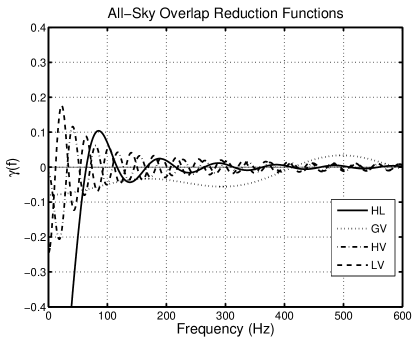
Figure 1: The overlap reduction functions for pairs of detector sites. Note that the ORF for the two LIGO sites goes off the scale of this plot at 40 Hz, which is the “seismic wall” below which LIGO data are too noisy to be of any use. The proximity and alignment of LLO and LHO makes HL the most favourable pair of detector sites for observations below 150 Hz or so. However, the proximity of the Virgo and GEO600 sites means the GV ORF is substantial out to higher frequencies, overcoming the low-frequency suppression due to their poor alignment. On the other hand, as shown in Table 1 the HV and LV ORFs, while they oscillate rapidly with increasing frequency, do not decay as precipitously as the HL ORF, making them more favourable than HL (but less than GV) for $f\gtrsim 200\mathrm{\,Hz}$.

2.2 Definition of Sensitivity

The strength of an isotropic stochastic background can be written in terms of the one-sided power spectral density $S_{\hbox{\scriptsize\rm gw}}(f)$ it would generate in an IFO with perpendicular arms.

The standard cross-correlation method seeks to measure the amplitude $S_{R}=S_{\hbox{\scriptsize\rm gw}}(f)/\mathcal{S}(f)$ of a background whose $S_{\hbox{\scriptsize\rm gw}}(f)$ is assumed to have a specified shape $\mathcal{S}(f)$. Given coïncident data between times $t_{1}$ and $t_{2}$ from detectors with one-sided noise power spectral densities (PSDs) $P_{1,2}(f)$, we can make an optimally-filtered cross-correlation statistic

$$Y=\int_{t_{1}}^{t_{2}}\int_{t_{1}}^{t_{2}}s_{1}(t)\,Q(t-t^{\prime})\,s_{2}(t)\,dt\,dt^{\prime}$$ (5)

with the optimal filter defined by its Fourier transform

$$\widetilde{Q}(f)=\mathcal{N}\frac{\gamma_{12}(f)\mathcal{S}(f)}{P_{1}(f)P_{2}(f)}$$ (6)

and $\mathcal{N}$ chosen so that $\langle Y\rangle=S_{R}$. If the geometric mean of the noise PSDs is large compared to $S_{\hbox{\scriptsize\rm gw}}(f)$, the expected variance of the statistic will be

$$\sigma^{2}=\frac{1}{2T}\left(\int_{0}^{\infty}\frac{\left[\gamma_{12}(f)\,\mathcal{S}(f)\right]^{2}}{P_{1}(f)\,P_{2}(f)}\right)^{-1}$$ (7)

where $T=t_{2}-t_{1}$ is the duration of the data analysed. The squared signal-to-noise ratio of the standard cross-correlation statistic will thus be

$$\mathrm{SNR}^{2}:=\frac{\langle Y\rangle^{2}}{\sigma^{2}}=2T\,S_{R}^{2}\int_{0}^{\infty}[\mathcal{S}(f)]^{2}\mathcal{I}_{12}(f)\ df\ ,$$ (8)

where we have defined a “sensitivity integrand” which illustrates the contribution to the sensitivity of different frequencies:

$$\mathcal{I}_{12}(f)=\frac{[\gamma_{12}(f)]^{2}}{P_{1}(f)\,P_{2}(f)}$$ (9)

We plot $\mathcal{I}(f)$ for several pairs of detectors in Figure 2, using the design sensitivities in[3, 4, 5].

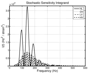
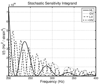
Figure 2: Sensitivity integrands $\mathcal{I}(f)$ for pairs of detector sites, where pairs like HL include e.g., the combined sensitivity of H1-L1 and H2-L1. To get an overall sensitivity, these need to be multiplied by the square of the shape of the SGWB spectrum $S_{\hbox{\scriptsize\rm gw}}(f)$. The HL pair is the most sensitive for flat and low-frequency spectra, but as shown in the closeup at the right, above 200 Hz, pairs involving Virgo are more sensitive when all detectors are operating at their design sensitivities. The GH and GL pairs are not shown, since the GEO600 noise spectrum [5] means that only the GV pair contributes significantly to the overall sensitivity at these frequencies.

As shown in [6], the optimal method for combining correlation measurements from different detector pairs is the same as that for combining measurements from different times: average the point estimates $Y$ with a relative weighting of $\sigma^{-2}$, and the resulting variance will be the inverse of the sum of the $\sigma^{-2}$ values. This produces a sensitivity integrand which is the sum of the integrands for individual pairs:

$$\mathcal{I}(f)=\sum_{\hbox{\scriptsize\rm pair}}\mathcal{I}_{\hbox{\scriptsize\rm pair}}(f)\ .$$ (10)

An immediate application of this is to define sensitivity integrands that combine pairs involving H1 and H2, e.g., $\mathcal{I}_{\hbox{\scriptsize\rm HL}}=\mathcal{I}_{\hbox{\scriptsize\rm H1,L1}}+\mathcal{I}_{\hbox{\scriptsize\rm H2,L1}}$. This is the same as using the spectrum of an optimally combined H pseudo-detector as described in [7].

Figure 3 shows the combined sensitivity for four networks of detectors operating at design sensitivity: the existing H-L network, an H-L-G network in which GEO600 is also operating at design sensitivity, and H-L-V and H-L-V-G networks which also include a design-sensitivity Virgo. The H1-H2 pair is not included in these networks, because the presence of correlated environmental noise necessitates special treatment of this pair [8].

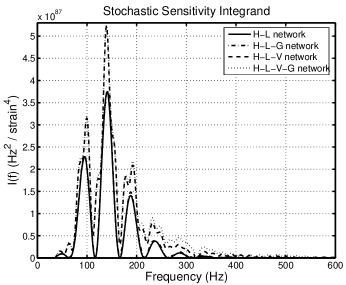
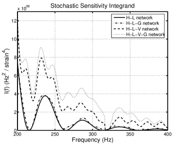
Figure 3: Combined sensitivity integrands for networks of detectors. In each case a network including “H” includes correlations between both H1 and H2 and the detectors at other sites. As the closeup on the right shows, addition of the LV, HV and GV pairs to the HL network increases sensitivity to backgrounds with significant power above 200 Hz.

Since the power in the faintest detectable “white” stochastic background is proportional to the square root of the area under the sensitivity integrand, we see that the addition of Virgo to the LHO-LLO network would be most useful in improving sensitivity to a narrow-band background peaked above 200 Hz, or to one whose spectrum rises with increasing frequency. As an illustration, Table 2 shows for several detector networks the faintest detectable background with constant $S_{\hbox{\scriptsize\rm gw}}(f)$ in a 100 Hz band, assuming one year of observation time and an SNR threshold of 3.29, associated with 5% false alarm and false dismissal rates.

Table 2: Smallest detectable band-limited background using each of the detector networks defined in Fig. 3. In each case, this is the strain power spectrum, in units of $10^{-48}\mathrm{\,Hz}^{-1}$, that could be detected with 5% false alarm and 5% false dismissal rates, using one year of coïncident data at design sensitivity.

Band	H-L	H-L-G	H-L-V	H-L-V-G
200–300 Hz	5.79	5.43	3.44	3.04
300–400 Hz	18.57	15.37	7.92	5.88

3 Simulations

To test cross-correlation analyses of LIGO and Virgo data, we injected a simulated SGWB signal into simulated LIGO and Virgo noise. The simulated noise data were the 24 hours of H1, H2, L1, and V1 data, all at nominal design sensitivity, initially generated for simulated searches for GW bursts and inspiralling compact object binaries [9, 10], known as “project 1b”. We chose a spectral shape designed to highlight the performance of the LV and HV pairs at $f\gtrsim 200\mathrm{\,Hz}$, but which corresponds to a model of an astrophysical SGWB. The spectrum we used is associated with the superposition of the tri-axial emission from the extra-galactic population of spinning magnetars with type I superconducting interior, as described in model B of [11], but updated using the star formation history of [12].

In Figure 4 we show the spectrum and the associated sensitivity integrand in the corresponding detectors. Since this spectrum rises with increasing frequency up to about 400 Hz, it is useful for illustrating the utility of a network involving Virgo to search for a broad-band astrophysical source.

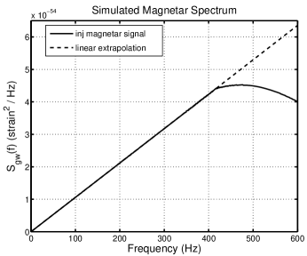
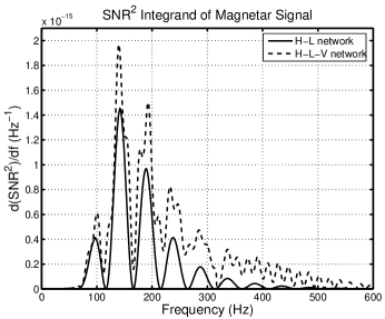
Figure 4: The magnetar spectrum used to generate simulated signals, and the associated integrand for squared signal-to-noise-ratio. Note that since $S_{\hbox{\scriptsize\rm gw}}(f)$ increases approximately linearly with frequency up to about 400 Hz, this spectrum, while broad-band, tends to favour the higher frequencies where LIGO-Virgo detector pairs are more sensitive. Beyond 400 Hz, the spectrum is no longer linear, but we show the SNR that would result from attempting to detect it with a $\mathcal{S}(f)\propto f$ filter; the corrections are negligible below about 500 Hz, and still small throughout the frequency range displayed. Note that integrating the area under the H-L-V curve on the right still gives an SNR below $10^{-6}$ from 24 hours of data, so we scale up the injected strain signal by a factor of several thousand in the simulations described in Section 4.

Since the model signal would be too weak to detect with first-generation interferometers, we scale up the signal strength, injecting a signal with the same spectral shape, but a much larger amplitude, in our simulations.

3.1 Simulation algorithm

The problem of simulation of the signal in a pair of detectors due to an isotropic and Gaussian SGWB has been considered previously in e.g., [6, 13, 14]. For this work we generalise that to a network of $N$ GW detectors. We need to satisfy (1) for each pair of detectors; treating $\{h_{A}(f)\}$ as the elements of a column vector $\mathbf{\widetilde{h}}(f)$ and $\{\gamma_{AB}(f)\}$ as the elements of a real, symmetric matrix $\boldsymbol{\gamma}(f)$, we can write this as a matrix equation

$$\langle\mathbf{\widetilde{h}}(f)\,\mathbf{\widetilde{h}}(f^{\prime})^{\dagger}\rangle=\frac{1}{2}S_{\hbox{\scriptsize\rm gw}}(f)\boldsymbol{\gamma}(f)\delta(f-f^{\prime})$$ (11)

If we can define a matrix $\boldsymbol{\beta}(f)$ which factors $\boldsymbol{\gamma}(f)$:

$$\boldsymbol{\gamma}(f)=\boldsymbol{\beta}(f)\boldsymbol{\beta}(f)^{\dagger}\ ,$$ (12)

then we can generate $N$ independent white noise data streams $\{\widetilde{\eta}_{A}(f)\}$ which satisfy

$$\langle\boldsymbol{\widetilde{\eta}}(f)\,\boldsymbol{\widetilde{\eta}}(f^{\prime})^{\dagger}\rangle=\boldsymbol{1}\delta(f-f^{\prime})$$ (13)

and then convert them into the desired coloured correlated data streams via

$$\mathbf{\widetilde{h}}(f)=\sqrt{\frac{S_{\hbox{\scriptsize\rm gw}}(f)}{2}}\boldsymbol{\beta}(f)\boldsymbol{\widetilde{\eta}}(f)$$ (14)

For a given $\boldsymbol{\gamma}(f)$, there are different choices of $\boldsymbol{\widetilde{\eta}}(f)$ which achieve the factorisation (12).

Since (11) is a covariance matrix, it is positive semi-definite, from which it follows (since $S_{\hbox{\scriptsize\rm gw}}(f)>0$) that $\boldsymbol{\gamma}(f)$ is positive semidefinite as well. $\boldsymbol{\gamma}(f)$ could have one or more zero eigenvalues in the presence of linear dependence between detector outputs. A practical example of this is two detectors sharing the same geometry and location, such as H1 and H2, are included in the network. We avoid this problem by generating a simulated signal for H1 and injecting it into both H1 and H2.

In the generic case where $\boldsymbol{\gamma}(f)$ is positive definite, we can make the straightforward choice of the Cholesky decomposition[15], in which $\boldsymbol{\beta}(f)$ is a lower diagonal matrix. In the case $N=2$, this reduces to the form used in e.g.,[6]. For $N=3$, if the diagonal elements of $\boldsymbol{\gamma}(f)$ are unity, the explicit form is

$$\boldsymbol{\beta}(f)=\left(\begin{array}[]{ccc}1&0&0\\ \gamma_{12}&\sqrt{1-\gamma_{12}^{2}}&0\\ \gamma_{13}&\frac{\gamma_{23}-\gamma_{12}\gamma_{13}}{\sqrt{1-\gamma_{12}^{2}}}&\sqrt{\frac{1+2\gamma_{12}\gamma_{13}\gamma_{23}-\gamma_{12}^{2}-\gamma_{13}^{2}-\gamma_{23}^{2}}{1-\gamma_{12}^{2}}}\end{array}\right)$$ (15)

However in practice we can simply use a fast iterative algorithm for the Cholesky decomposition.

Other factorisation strategies which treat the different detectors more symmetrically (e.g., defining $\boldsymbol{\beta}(f)=\boldsymbol{\Lambda}(f)^{1/2}\mathbf{U}(f)$ where $\boldsymbol{\Lambda}(f)$ is the diagonal matrix of eigenvalues of $\boldsymbol{\gamma}(f)$ and $\mathbf{U}(f)$ is the matrix constructed from the corresponding eigenvectors) may be more demanding in terms of computational power, but more numerically stable when correlations between the detectors are large and off-diagonal elements of $\boldsymbol{\gamma}(f)$ are comparable to unity. In particular, this strategy can deal directly with the case when $\boldsymbol{\gamma}(f)$ has one or more zero eigenvalues.

3.2 Filtering strategy

The continuous frequency-domain idealisation (14) needs to be applied with care to finite stretches of real detector data. In the time domain, the multiplication (14) amounts to a convolution

$$\mathbf{h}(t)=\int_{-\infty}^{\infty}\mathbf{K}(t-t^{\prime})\,\boldsymbol{\eta}(t^{\prime})\,dt^{\prime}$$ (16)

with a kernel which is the inverse Fourier transform of

$$\mathbf{\widetilde{K}}(f)=\sqrt{\frac{S_{\hbox{\scriptsize\rm gw}}(f)}{2}}\boldsymbol{\beta}(f)\ .$$ (17)

If the time-domain kernel $\mathbf{K}(\tau)$ is negligible outside the interval $-\tau_{-}<\tau<\tau_{+}$, we can use the standard overlap-and-add strategy to generate a continuous stream of time-series data, as illustrated in Figure 5:

Figure 5: The overlap-and-add algorithm.

1. Generate a sequence of “buffers” of white noise data for each of the $N$ detectors, each of length $T$.

2. Convolve each buffer with the kernel $\mathbf{K}(\tau)$ to obtain a time series of length $\tau_{-}+T+\tau_{+}$, with an associated start time $\tau_{-}$ before the start and end time $\tau_{+}$ after the end of the original buffer. (This is most naturally done in the frequency domain, zero-padding the white noise by $\tau_{-}$ at the beginning and $\tau_{+}$ at the end, then Fourier transforming and multiplying by $\mathbf{\widetilde{K}}(f)$ before inverse-Fourier-transforming.)

3. Add together the processed data buffers, overlapping by $\tau_{+}$ on one end and $\tau_{-}$ on the next, producing correlated coloured time-series data of duration $T$ times the number of buffers, plus transients of $\tau_{-}$ at the beginning and $\tau_{+}$ at the end, which are discarded.

This strategy was implemented in code based on Virgo’s “Noise Analysis Package” (nap) [16].

4 Analysis of simulated data

The continuous signals described in Section 3 were injected into the “project 1b” simulated noise and the resulting time series analysed using the matapps stochastic analysis code developed by the LSC. [17]. In particular, the cross-correlation (5) was performed in the frequency domain without any need to resample the time-series data, using a variation of the method described in [18] and applied in [14]. Several simulation runs were performed in which same set of simulated signals were injected into the four data streams, scaled up by a different factor for each run. The results of two of those simulations are shown here. In Figure 6 we plot the individual point estimates and error bars in each of the five detector pairs (every combination except for H1-H2). The amplitude measure $S_{R}$ quoted is the one-sided strain PSD at 200 Hz.

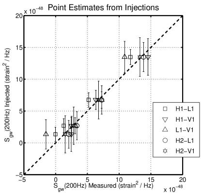
Figure 6: The individual point estimates and one-sigma error bars with signals injected at two different levels. The strength of the injection is shown on the vertical axis, as a strain power at 200 Hz, while the estimate of this quantity from each detector pair is on the horizontal axis. The error bars are drawn vertically for ease of reading, and because they are frequentist error bars as quoted. Note that the signals are seen at comparable strength in all five pairs of detectors.

The optimal filter used assumed the shape $\mathcal{S}(f)\propto f$, although the injected signals only had that form below about 400 Hz. The analysis was done over a frequency band 50–500 Hz to avoid difficulties arising from this mismatch, as illustrated in Figure 4.

The optimal combination of these results is shown in Table 3, both for the full network and for the network consisting only of the two LHO-LLO pairs. Our error bars are reduced by 15% via the inclusion of the LIGO-Virgo pairs. Note that although this source has more power at the intermediate frequencies favoured by the LIGO-Virgo pairs, it is still broad-band. A narrow-banded source with most of its power above 200 Hz would favour LIGO-Virgo pairs to an even greater extent.

$S_{\hbox{\scriptsize\rm gw}}(200\mathrm{\,Hz})$ ($10^{-48}\mathrm{\,Hz}^{-1}$)
Injected	H-L Result	H-L-V Result
$1.35$	$0.39\pm 0.98$	$0.43\pm 0.82$
$2.70$	$1.69\pm 0.99$	$2.31\pm 0.67$
$6.74$	$5.63\pm 1.02$	$6.29\pm 0.69$
$13.49$	$12.22\pm 1.06$	$12.35\pm 0.88$

Table 3: The values of $S_{\hbox{\scriptsize\rm gw}}(200\mathrm{\,Hz})$ calculated from the simulated project 1b data, with associated one-sigma error bars, for the H-L network consisting of the H1-L1 and H2-L1 pairs, and for the H-L-V network consisting of those plus the H1-V1, H2-V1, and L1-V1 pairs. We see that including Virgo in the network reduces our error bars for this broad-band astrophysical spectrum by 15%.

5 Conclusions and Outlook

We have demonstrated how the inclusion of LIGO-Virgo and possibly GEO600-Virgo detector pairs can enhance the sensitivity of the global GW detector network to an isotropic background of gravitational waves, particularly at frequencies above 200 Hz. As a practical illustration, we have adapted and applied pipelines for generating correlated simulated signals in the LSC and Virgo detectors, and for analysing coïncident data via the standard cross-correlation technique. The specific astrophysical model we used (which was chosen because its frequency spectrum was peaked at frequencies where LIGO-Virgo pairs at design will be more sensitive than LLO-LHO pairs) had to have its amplitude increased to be detectable by any pair of first-generation IFOs. Nonetheless, the exercise illustrates how multiple detector pairs can be used to discover an “unexpected” background.

Virgo is not yet at its nominal design sensitivity, but has improved its sensitivity markedly over the past year, and its first full science run starts in May 2007, to be analysed in conjunction with the end of LIGO’s S5 run.

References

References

- [1] Flanagan É É 1993 Phys. Rev.D48 2389; astro-ph/9305029
- [2] Whelan J T 2006 Class. Quantum Grav.23 1181; gr-qc/0509109
- [3] A. Lazzarini and R. Weiss, technical document LIGO-E950018-02-E (1996). Digital format from http://www.ligo.caltech.edu/jzweizig/distribution/LSC_Data/
- [4] M Punturo, Virgo note VIR-NOT-PER-1390-51, Issue 10 (2004). Digital format from http://www.virgo.infn.it/senscurve/
- [5] GEO-600 Theoretical Noise Budget, version 4.0 with 250 Hz signal detuning, available from http://www.geo600.uni-hannover.de/geocurves/
- [6] Allen B and Romano J D 1999 Phys. Rev.D59 102001; gr-qc/9710117.
- [7] Lazzarini A et al 2004 Phys. Rev.D70 062001; gr-qc/0403093
- [8] Fotopoulos N V for the LIGO Scientific Collaboration 2006 Class. Quantum Grav.23 S693
- [9] Beauville F et al (LIGO-Virgo Working Group), submitted to Phys. Rev.D; gr-qc/0701026
- [10] Beauville F et al (LIGO-Virgo Working Group), submitted to Phys. Rev.D; gr-qc/0701027
- [11] Regimbau T. and de Freitas Pacheco J. A. 2006 A&A 447 1
- [12] Hopkins A.M. and Beacom J. 2006 ApJ in press; e-print: astro-ph/0601463
- [13] Bose S et al, Class. Quantum Grav.20 S677 (2003)
- [14] Abbott B et al (LIGO Scientific Collaboration), submitted to Phys. Rev.D; gr-qc/0703068
- [15] Golub G H and Van Loan C F 1989 Matrix Computations (Johns Hopkins Univ Press, Baltimore)
- [16] http://wwwcascina.virgo.infn.it/DataAnalysis/Noise/nap_index.html
- [17] http://www.lsc-group.phys.uwm.edu/daswg/projects/matapps.html
- [18] Whelan J T et al 2005 Class. Quantum Grav.22 S1087; gr-qc/0506025