On Loops in the Hyperbolic Locus
of the Complex Hénon Map
and Their Monodromies

Abstract.

We prove John Hubbard’s conjecture on the topological complexity of the hyperbolic horseshoe locus of the complex Hénon map. Indeed, we show that there exist several non-trivial loops in the locus which generate infinitely many mutually different monodromies. Our main tool is a rigorous computational algorithm for verifying the uniform hyperbolicity of chain recurrent sets. In addition, we show that the dynamics of the real Hénon map is completely determined by the monodromy of a certain loop, providing the parameter of the map is contained in the hyperbolic horseshoe locus of the complex Hénon map.

1. Introduction

One of the motivations of this work is to give an answer to the conjecture of John Hubbard on the topology of hyperbolic horseshoe locus of the complex Hénon map

$$H_{a,c}:\mathbb{C}^{2}\to\mathbb{C}^{2}:\begin{pmatrix}x\\ y\end{pmatrix}\mapsto\begin{pmatrix}x^{2}+c-ay\\ x\end{pmatrix}.$$

Here $a$ and $c$ are complex parameters.

We describe the conjecture following a formulation given by Bedford and Smillie [5].

Let us define

$$K_{a,c}^{\mathbb{C}}:=\{p\in\mathbb{C}^{2}:\{H_{a,c}^{n}(p)\}_{n\in\mathbb{Z}}\text{ is bounded}\},\quad K_{a,c}^{\mathbb{R}}:=K_{a,c}^{\mathbb{C}}\cap\mathbb{R}^{2}.$$

The set $K_{a,c}^{\mathbb{C}}$ is compact and invariant with respect to $H_{a,c}$. When the parameters $a$ and $c$ are both real, the real plane $\mathbb{R}^{2}\subset\mathbb{C}^{2}$ is invariant and hence so is $K_{a,c}^{\mathbb{R}}$. In this case, we regard $H_{a,c}$ also as a dynamical system defined on $\mathbb{R}^{2}$ and call it the real Hénon map.

Our primary interest is on the parameter space, especially the set of parameters such that the complex and real Hénon maps become a uniformly hyperbolic horseshoe. More precisely, we study the following sets:

$$\mathcal{H}^{\mathbb{C}}:=\{(a,c)\in\mathbb{C}^{2}:H_{a,c}|{K_{a,c}^{\mathbb{C}}}\text{ is a hyperbolic full horseshoe}\},$$

$$\mathcal{H}^{\mathbb{R}}:=\{(a,c)\in\mathbb{R}^{2}:H_{a,c}|{K_{a,c}^{\mathbb{R}}}\text{ is a hyperbolic full horseshoe}\}.$$

By a hyperbolic full horseshoe, we mean an uniformly hyperbolic invariant set which is topologically conjugate to the full shift map $\sigma$ defined on $\Sigma_{2}=\{0,1\}^{\mathbb{Z}}$, the space of bi-infinite sequences of two symbols.

A classical result of Devaney and Nitecki [12] claims that if $(a,c)$ is in

$$\mathrm{DN}:=\{(a,c)\in\mathbb{R}^{2}:c<-(5+2\sqrt{5})\,(|a|+1)^{2}/4,\,a\neq 0\}$$

then $K_{a,c}^{\mathbb{R}}$ is a hyperbolic full horseshoe. Thus $\mathrm{DN}\subset\mathcal{H}^{\mathbb{R}}$ holds. They also showed that the set

$$\mathrm{EMP}:=\{(a,c)\in\mathbb{R}^{2}:c>(|a|+1)^{2}/4\}$$

consists of parameter values such that $K_{a,c}^{\mathbb{R}}=\emptyset$. Later, Hubbard and Oberste-Vorth investigated the Hénon map form the point of view of complex dynamics and improved the hyperbolicity criterion by showing that

$$\mathrm{HOV}:=\{(a,c)\in\mathbb{C}^{2}:|c|>2(|a|+1)^{2},\,a\neq 0\}$$

is included in $\mathcal{H}^{\mathbb{C}}$. Remark that $\mathrm{EMP}\cap\mathrm{HOV}$ is non-empty. In this parameter region, although $K_{a,c}^{\mathbb{C}}$ is a full horseshoe, it does not intersect with $\mathbb{R}^{2}$.

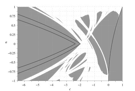
Figure 1. The shaded regions consist of hyperbolic (not necessarily full horseshoe) parameters of the real Hénon map.

Figure 1 illustrates a subset of parameter values on which the chain recurrent set of the real Hénon map is uniformly hyperbolic (not necessarily a full horseshoe) [1]. Three solid lines are parts of the boundaries of $\mathrm{DN}$, $\mathrm{HOV}$ and $\mathrm{EMP}$, from left to right. On the biggest island to the left, the chain recurrent set coincides with $K_{a,c}^{\mathbb{R}}$ and is conjugate to the full shift. Hence the island is contained in $\mathcal{H}^{\mathbb{R}}$.

We then consider the relation between $\mathcal{H}^{\mathbb{R}}$ and $\mathcal{H}^{\mathbb{C}}$. By the result of Bedford, Lyubich and Smillie [3, Theorem 10.1], we have $\mathcal{H}^{\mathbb{R}}\subset\mathcal{H}^{\mathbb{C}}\cap\mathbb{R}^{2}$. It is then natural to ask what happens in the rest of $\mathcal{H}^{\mathbb{C}}\cap\mathbb{R}^{2}$.

To be specific, we divide $\mathcal{H}^{\mathbb{C}}\cap\mathbb{R}^{2}$ into three mutually disjoint sets.

Definition 1 (Bedford and Smillie [5]).

We call $(a,c)\in\mathcal{H}^{\mathbb{C}}\cap\mathbb{R}^{2}$ is of type-1 if $(a,c)\in\mathcal{H}^{\mathbb{R}}$, and of type-2 if $K_{a,c}^{\mathbb{R}}=\emptyset$. Otherwise, it is of type-3.

Since $\mathrm{DN}\subset\mathcal{H}^{\mathbb{R}}$, the set of type-1 parameter values is non-empty. The set of type-2 parameter values is also non-empty since it contains $\mathrm{EMP}\cap\mathrm{HOV}$. However, the existence of a type-3 parameter value was open.

Conjecture 1 (Hubbard).

There exists a parameter value of type-3.

As we will see later, this conjecture turned to be true.

Besides the existence, Hubbard also conjectured that there are infinitely many classes of type-3 parameter values corresponding to mutually different real dynamics. This stronger conjecture is, to be precise, given in terms of the monodromy representation of the fundamental group of the hyperbolic horseshoe locus as follows.

Denote by $\mathcal{H}^{\mathbb{C}}_{0}$ the component of $\mathcal{H}^{\mathbb{C}}$ that contains $\mathrm{HOV}$. Let us fix a basepoint $(a_{0},c_{0})\in\mathrm{DN}$ and a topological conjugacy $h_{0}:K_{a_{0},c_{0}}^{\mathbb{C}}\to\Sigma_{2}$.

Given a loop $\gamma:[0,1]\to\mathcal{H}^{\mathbb{C}}_{0}$ based at $(a_{0},c_{0})$, we construct a continuous family of conjugacies $h_{t}^{\gamma}:K_{\gamma(t)}^{\mathbb{C}}\to\Sigma_{2}$ along $\gamma$ such that $h_{0}^{\gamma}=h_{0}$ (see §4 for the details). This is possible because $K_{a,c}^{\mathbb{C}}$ is uniformly hyperbolic along $\gamma$. When no confusion may result we suppress $\gamma$ and write $h_{t}^{\gamma}$ as $h_{t}$. Finally we set $\rho(\gamma):=h_{1}\circ(h_{0})^{-1}$. It is easy to see that $\rho$ defines a group homomorphism

$$\rho:\pi_{1}(\mathcal{H}^{\mathbb{C}}_{0},(a_{0},c_{0}))\to\operatorname{Aut}(\Sigma_{2})$$

where $\operatorname{Aut}(\Sigma_{2})$ is the group of the automorphisms of $\Sigma_{2}$. Recall that an $automorphism$ of $\Sigma_{2}$ is a homeomorphism of $\Sigma_{2}$ which commutes with the shift [18]. We call $\rho$ the monodromy homomorphism and denote its image by $\Gamma$.

For example, let $\gamma_{\emptyset}$ be a loop in $\mathcal{H}^{\mathbb{C}}_{0}$ based at $(a_{0},c_{0})$ and homotopic to the generator of $\pi_{1}(\mathrm{HOV})$. It is then shown [5] that $\rho(\gamma_{\emptyset})$ is an involution which interchanges the symbols $0$ and $1$. Namely, $(\rho(\gamma_{\emptyset})(s))_{i}=1-s_{i}$ for all $s=(s_{i})\in\{0,1\}^{\mathbb{Z}}$.

The monodromy homomorphism was originally defined for polynomial maps of one complex variable. In this case, since the map does not have the inverse, the target space of the monodromy homomorphism is the automorphism group of one-sided shift space of $d$-symbols, where $d$ is the degree of the polynomial. When $d=2$, this group is isomorphic to $\mathbb{Z}_{2}$ and the monodromy homomorphism is shown to be surjective since it maps the generator of $\pi_{1}(\mathbb{C}\setminus\{\text{the Mandelbrot set}\})$ to $1\in\mathbb{Z}_{2}$. The monodromy homomorphism is also surjective even when $d>2$, although the proof is much harder than the case $d=2$ because the automorphism group becomes much more complicated [6].

Hubbard conjectured that the surjectivity also holds in the case of the complex Hénon map.

Conjecture 2 (Hubbard).

The monodromy homomorphism $\rho$ is surjective, that is, $\Gamma=\operatorname{Aut}(\Sigma_{2})$.

The structure of $\operatorname{Aut}(\Sigma_{2})$ is quite complicated [7]: it contains every finite group; furthermore, it contains the direct sum of any countable collection of finite groups; and it also contains the direct sum of countably many copies of $\mathbb{Z}$. Therefore, the conjecture implies, provided it is true, that the topological structure of $\mathcal{H}^{\mathbb{C}}$ is very rich, in contrast to the one-dimensional case where the fundamental group of $\mathbb{C}\setminus\{\text{the Mandelbrot set}\}$ is simply $\mathbb{Z}$.

Let us state the main results of the paper now.

First, we claim that Conjecture 1 is true.

Theorem 1.

There exist parameter values of type-3. In fact, if $(a,c)$ is in one of the following sets:

$$I_{p}:=\{1\}\times[-5.46875,-5.3125], I_{q}:=\{0.25\}\times[-2.296875,-2.21875],$$

$$I_{r}:=\{-1\}\times[-5.671875,-4.4375], I_{s}:=\{-0.375\}\times[-2.15625,-1.8125]$$

then $(a,c)$ is of type 3.

As far as Conjecture 2 is concerned, we obtain the following result.

Theorem 2.

The order of the group $\Gamma$ is infinite. In particular, it contains an element of infinite order.

Apart form the theoretical interest, the monodromy theory of complex Hénon map can contribute to the understanding of the real Hénon map.

Let $(a,c)\in\mathcal{H}^{\mathbb{C}}\cap\mathbb{R}^{2}$. If $(a,c)$ is of type-1 or 2, then by definition $K^{\mathbb{R}}_{a,c}$ is a full horseshoe, or the empty set. Suppose $(a,c)$ is of type-3. We then ask what $K^{\mathbb{R}}_{a,c}$ can be. By definition, $K^{\mathbb{R}}_{a,c}$ is a proper subset of $K_{a,c}^{\mathbb{C}}\cong\Sigma_{2}$. The uniform hyperbolicity implies the existence of a Markov partition for $K^{\mathbb{R}}_{a,c}$, and therefore, $K^{\mathbb{R}}_{a,c}$ must be topologically conjugate to some subshift of finite type. The following theorem reveals that $K^{\mathbb{R}}_{a,c}$ is actually a subshift of $\Sigma_{2}$ which is realized as the fixed point set of the monodromy of a loop passing through $(a,c)$.

Theorem 3.

For any $(a,c)\in\mathcal{H}_{0}^{\mathbb{C}}\cap\mathbb{R}^{2}$, there exists a loop $\gamma:[0,1]\to\mathcal{H}_{0}^{\mathbb{C}}$ with $\gamma(1/2)=(a,c)$ such that $H_{a,c}:K_{a,c}^{\mathbb{R}}\to K_{a,c}^{\mathbb{R}}$ is topologically conjugate to

$$\sigma|_{\operatorname{Fix}(\rho(\gamma))}:\operatorname{Fix}(\rho(\gamma))\to\operatorname{Fix}(\rho(\gamma)).$$

In fact, it suffice to set $\gamma:=\bar{\alpha}^{-1}\cdot\alpha$, where $\alpha$ is an arbitrary path in $\mathcal{H}_{0}^{\mathbb{C}}$ that starts at a point in $\mathrm{DN}$ and ends at $(a,c)$. Here $\bar{\alpha}$ denotes the complex conjugate of $\alpha$. The conjugacy is given by the restriction of $h_{1/2}$ to $K^{\mathbb{R}}_{a,c}$. Namely, the following diagram commutes.

$$\begin{CD}K^{\mathbb{R}}_{a,c}@>{H_{a,c}}>{}>K^{\mathbb{R}}_{a,c}\\ @V{h_{1/2}}V{\cong}V@V{\cong}V{h_{1/2}}V\\ \operatorname{Fix}(\rho(\gamma))@>{\sigma}>{}>\operatorname{Fix}(\rho(\gamma)).\end{CD}$$

As an application of Theorem 3, we obtain the following.

Theorem 4.

Let $(a,c)\in I_{p}$. The real Hénon map $H_{a,c}:K_{a,c}^{\mathbb{R}}\to K_{a,c}^{\mathbb{R}}$ is topologically conjugate to the subshift of $\Sigma_{2}$ with two forbidden blocks $0010100$ and $0011100$. Similarly, $K_{a,c}^{\mathbb{R}}$ is conjugate to the subshift of $\Sigma_{2}$ defined the following forbidden blocks: $10100$ and $11100$ for $(a,c)\in I_{q}$; $10010$ and $10110$ for $(a,c)\in I_{r}$; $0010$ and $0110$ for $(a,c)\in I_{s}$.

Notice that $I_{p}$ contains $(a,c)=(1,-5.4)$, the parameter studied by Davis, MacKay and Sannami [10]. The subshift for $(a,c)\in I_{p}$ given in Theorem 4 is equivalent to that observed by them. Thus, we can say that their observation is now rigorously verified. We also remark that this theorem is closely related to the so-called “pruning front” theory [9, 10]. Theorem 3 implies that “primary pruned regions”, or, “missing blocks” of $K_{a,c}^{\mathbb{R}}$ is nothing else but the region where the exchange of symbols occurs along $\gamma$.

The structure of the paper is as follows. We prove the theorems in Section 2, leaving computational algorithms to Section 3 and 4. In Section 3, we summarize the algorithm for proving uniform hyperbolicity developed by the author [1]. Section 4 is devoted to an algorithm for computing the monodromy homomorphism. In the appendix, we discuss a method for rigorously counting the number of periodic points, which gives rise to an alternative proof of Theorem 1. Programs for computer assisted proofs are available at the author’s pweb page (http://www.math.kyoto-u.ac.jp/~arai/).

The author is grateful, first of all, to John Hubbard, the originator of the problem. He also would like to thank E. Bedford, P. Cvitanović, S. Hruska, H. Kokubu, A. Sannami, J. Smillie, and S. Ushiki for many valuable suggestions.

2. Proofs

We first prove Theorem 3. The key is the symmetry of the Hénon map with respect to the complex conjugation [5]. By the symmetry we mean the equation

$$\phi\circ H_{a,c}=H_{\bar{a},\bar{c}}\circ\phi$$

where $\phi$ is the complex conjugation that maps $z=(x,y)$ to $\bar{z}=(\bar{x},\bar{y})$.

Proof of Theorem 3.

Take an arbitrary point $z\in K^{\mathbb{C}}_{a,c}$ and let

$$s_{z}:=h_{1/2}(z)\in\Sigma_{2}.$$

We will show that $\rho(\gamma)(s_{z})=s_{z}$ if and only if $z\in\mathbb{R}^{2}$. By abuse of notation, we denote the continuation of $z$ along $\gamma$ by

$$z(\gamma,t):=(h_{t})^{-1}(s_{z})\in\mathbb{C}^{2}.$$

Note that $z(\gamma,1/2)=z$. By the continuity of hyperbolic invariant sets, the map $t\mapsto(\gamma(t),z(\gamma,t))$ defines a continuous loop in $\mathbb{C}^{2}\times\mathbb{C}^{2}$.

Let $\bar{\gamma}:=\phi\circ\gamma$. The symmetry $\phi\circ H_{a,c}=H_{\bar{a},\bar{c}}\circ\phi$ implies that the complex conjugate of the continuation of $z$ along $\gamma$ is just the continuation of $\bar{z}=\phi(z)$ along $\bar{\gamma}$. That is, we have

$$\overline{z(\gamma,t)}=\bar{z}(\bar{\gamma},t).$$

By the construction, we have $\bar{\gamma}=\gamma^{-1}$ and hence $z(\bar{\gamma},t)=z(\gamma,1-t)$. Therefore,

$$\rho(\gamma)(s_{z})=h_{1}((h_{0})^{-1}(s_{z}))=h_{1}(z(\gamma,0))=h_{1}(\overline{z(\gamma,0)})$$

$$=h_{1}(\bar{z}(\bar{\gamma},0))=h_{1}(\bar{z}(\gamma,1))=h_{1}((h_{1})^{-1}(s_{\bar{z}})) =s_{\bar{z}}.$$

The third equality holds because $K_{\gamma(0)}^{\mathbb{C}}\subset\mathbb{R}^{2}$ and hence $z(\gamma,0)=\overline{z(\gamma,0)}$. Since the map $h_{1/2}$ is a bijection between $K_{a,c}^{\mathbb{C}}$ and $\Sigma_{2}$, it follows that $\rho(\gamma)(s_{z})=s_{z}$ if and only if $z=\bar{z}$. This proves the theorem. ∎

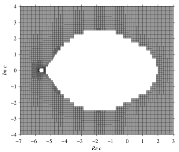
Figure 2. The shaded region is contained in $\mathcal{H}^{\mathbb{C}}\cap\{a=1\}$.

Figure 3. The shaded region is contained in $\mathcal{H}^{\mathbb{C}}\cap\{a=0.25\}$.

Figure 4. The shaded region is contained in $\mathcal{H}^{\mathbb{C}}\cap\{a=-1\}$.

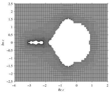
Figure 5. The shaded region is contained in $\mathcal{H}^{\mathbb{C}}\cap\{a=-0.375\}$.

Now we discuss Theorem 1. We begin by defining $I_{p}$, $I_{q}$, $I_{r}$ and $I_{s}$. Let

$$L_{p} :=\{1\}\times\{\mathbb{C}\setminus\text{white regions in Figure~{}\ref{FIG:ap}}\},$$

$$L_{q} :=\{0.25\}\times\{\mathbb{C}\setminus\text{white regions in Figure~{}\ref{FIG:a+025}}\},$$

$$L_{r} :=\{-1\}\times\{\mathbb{C}\setminus\text{white regions in Figure~{}\ref{FIG:ar}}\},$$

$$L_{s} :=\{-0.375\}\times\{\mathbb{C}\setminus\text{white regions in Figure~{}\ref{FIG:a-0375}}\}$$

and $L:=L_{p}\cup L_{q}\cup L_{r}\cup L_{s}$. To be precise, these regions are defined by a finite number of closed rectangles. The complete list of these rectangles is available at the author’s web page. The set $L_{p}\cap\mathbb{R}^{2}$ have three components: two unbounded intervals, and one bounded interval. We define $I_{p}$ to be this bounded one. Similarly, $I_{q}$, $I_{r}$ and $I_{s}$ are defined to be the bounded intervals contained in $L_{q}\cap\mathbb{R}^{2}$, $L_{q}\cap\mathbb{R}^{2}$ and $L_{s}\cap\mathbb{R}^{2}$, respectively.

Lemma 5.

If $(a,c)\in L$ then $H_{a,c}$ is uniformly hyperbolic on its chain recurrent set $\mathcal{R}(H_{a,c})$.

The proof of this lemma is computer assisted. We leave it to §3.

Recall that the hyperbolicity of the chain recurrent set implies the $\mathcal{R}$-structural stability [22, Corollary 8.24]. Therefore, it follows from Lemma 5 that no bifurcation occurs in $\mathcal{R}(H_{a,c})$ as long as $(a,c)\in L$. Thus $\mathcal{R}(H_{a,c})$ is a hyperbolic full horseshoe for all $(a,c)\in L$.

Lemma 5 is not sufficient to conclude the hyperbolicity of $K_{a,c}^{\mathbb{C}}$ because $\mathcal{R}(H_{a,c})$ and $K_{a,c}^{\mathbb{C}}$ do not necessarily coincide. However, we can show that these sets are equal in the horseshoe locus, as follows.

Corollary 6.

If $(a,c)\in L$ then $H_{a,c}|K_{a,c}^{\mathbb{C}}$ is a hyperbolic full horseshoe, that is, $L\subset\mathcal{H}^{\mathbb{C}}$.

Proof of Corollary 6.

Let

$$K_{a,c}^{+}:= \{p\in\mathbb{C}^{2}:\{H_{a,c}^{n}(p)\}_{n\geq 0}\text{ is bounded}\},$$

$$K_{a,c}^{-}:= \{p\in\mathbb{C}^{2}:\{H_{a,c}^{n}(p)\}_{n\leq 0}\text{ is bounded}\}$$

and $J_{a,c}^{\pm}:=\partial K_{a,c}^{\pm}$. Define $J_{a,c}=J_{a,c}^{+}\cap J_{a,c}^{-}$. Then $K_{a,c}^{\mathbb{C}}=K_{a,c}^{+}\cap K_{a,c}^{-}$ and we have $J_{a,c}\subset\mathcal{R}(H_{a,c})\subset K_{a,c}^{\mathbb{C}}$ [20, Proposition 9.2.6, Theorem 9.2.7]. Suppose $(a,c)\in L$. Since $\mathcal{R}(H_{a,c})$ is a full horseshoe, all periodic points of $H_{a,c}$ is contained in $\mathcal{R}(H_{a,c})$ and therefore they are of saddle type. Thus there exists no attracting periodic orbit. Furthermore, $J_{a,c}$ is uniformly hyperbolic because it is a closed sub-invariant set of $\mathcal{R}(H_{a,c})$. It follows that $\operatorname{int}K^{+}=\emptyset$ [4, Theorem 5.9]. Since $|a|\leq 1$, we also have $\operatorname{int}K^{-}=\emptyset$ [4, Lemma 5.5]. As a consequence, $J_{a,c}^{+}=K_{a,c}^{+}$ and $J_{a,c}^{-}=K_{a,c}^{-}$, and hence $J_{a,c}=\mathcal{R}(H_{a,c})=K_{a,c}^{\mathbb{C}}$. Therefore, Lemma 5 implies this corollary. ∎

From Corollary 6 it follows that $I_{p}$, $I_{q}$, $I_{s}$ and $I_{r}$ are contained in $\mathcal{H}_{0}^{\mathbb{C}}\cap\mathbb{R}^{2}$. To complete the proof of Theorem 1, we need to show that these intervals are of type-3.

A simple and direct way for proving this is to show that the number of periodic points contained in $K_{a,c}^{\mathbb{R}}$ is non-zero and different from that of a full horseshoe. Rigorous interval arithmetic and the Conley index theory can be applied for this purpose. We discuss this method in the appendix.

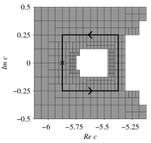
Figure 6. The loop $\beta_{p}:[0,1]\to L_{p}$ based at $(a,c)=(1,-5.875)$.

Another way is to make use of Theorem 3. Since we have already shown that $L\subset\mathcal{H}_{0}^{\mathbb{C}}$, we can consider the monodromy of loops in $L$, from which we derive the information of $K_{a,c}^{\mathbb{R}}$.

Let $\beta_{p}:[0,1]\to L_{p}$ be a loop that turns around the smaller white island of Figure 2 as illustrated in Figure 6. We require that $\beta_{p}(1/2)\in I_{p}$, and that $\beta_{p}$ be symmetric with respect to the complex conjugation, that is, $\bar{\beta}_{p}=\beta_{p}^{-1}$. Then we define a loop $\gamma_{p}:[0,1]\to L_{p}\cup\mathrm{HOV}$ based at $(1,-10)\in\mathrm{DN}$ by setting

$$\gamma_{p}:=\bar{\alpha}^{-1}\cdot\beta_{p}\cdot\alpha$$

where $\alpha:[0,1]\to\mathrm{HOV}\cup L_{p}$ is a path from $(1,-10)$ to the basepoint of $\beta_{p}$. Choose the parametrization of $\gamma_{p}$ so that $\gamma_{p}(1/2)\in I_{p}$ and $\bar{\gamma}_{p}=\gamma_{p}^{-1}$ hold. Similarly we define loops $\gamma_{q}$, $\gamma_{r}$ and $\gamma_{s}$ based at $(1,-10)$ turning around the smaller islands in $L_{q}$, $L_{r}$ and $L_{s}$, respectively.

Proposition 7.

The automorphism $\rho(\gamma_{p})$ interchanges the words $0010100$ and $0011100$ contained in $s=(s_{i})_{i\in\mathbb{Z}}\in\Sigma_{2}$. Namely,

$$(\rho(\gamma_{p})(s))_{i}=\begin{cases}0&\text{if }s_{i-3}\cdots s_{i}\cdots s_{i+3}=0011100\\ 1&\text{if }s_{i-3}\cdots s_{i}\cdots s_{i+3}=0010100\\ s_{i}&\text{otherwise.}\end{cases}$$

Similarly, $\rho(\gamma_{q})$ interchanges $10100$ and $11100$, $\rho(\gamma_{r})$ interchanges $10010$ and $10110$, and $\rho(\gamma_{s})$ interchanges $0010$ and $0110$.

The proof of Proposition 7 is also computer assisted. An algorithm for this will be discussed in §4.

Now we are prepared to prove Theorem 1.

Proof of Theorem 1.

Since $\operatorname{Fix}(\rho(\gamma_{p}))$ is a non-empty proper subset of $\Sigma_{2}$, Theorem 3 implies that $\gamma_{p}(1/2)\in I_{p}$ is of type-3. By considering loops homotopic to $\gamma_{p}$, we can show that all $(a,c)\in I_{p}$ are also of type-3. Proofs for other intervals are the same. ∎

Theorem 2 immediately follows from the following proposition.

Proposition 8.

The order of $\psi=\rho(\gamma_{\emptyset})\cdot\rho(\gamma_{s})$ is infinite.

The proof below is due to G. A. Hedlund [14, Theorem 20.1].

Proof.

For non-negative integer $p$, we define elements of $\Sigma_{2}$ named $x^{(2p)}$ and $x^{(2p+1)}$ by

$$x^{(2p)}=\cdots 01010101{\mathbf{0110110}}(10)^{p} .11111\cdots,$$

$$x^{(2p+1)}=\cdots 01010101{\mathbf{0110110}}(10)^{p}1 .00000\cdots.$$

We then look at the orbit of $x=x^{(0)}$ under the map $\psi$. A simple calculation shows that

$$x=\,\cdots 01010101{\mathbf{0110110}}.11111\cdots =x^{(0)},$$

$$\psi(x)=\,\cdots 1010101{\mathbf{0110110}}1.00000\cdots =x^{(1)},$$

$$\psi^{2}(x)=\,\cdots 010101{\mathbf{0110110}}10.11111\cdots =x^{(2)},$$

$$\psi^{3}(x)=\,\cdots 10101{\mathbf{0110110}}101.00000\cdots =x^{(3)}.$$

By induction, it follows that $\psi^{n}(x^{(0)})=x^{(n)}$. Since $x^{(n)}\neq x^{(m)}$ if $n\neq m$, this implies that the order of $\psi$ is infinite. ∎

Theorem 4 is a direct consequence of Theorem 3 and Proposition 7.

3. Hyperbolicity

We recall an algorithm for proving the uniform hyperbolicity of chain recurrent sets developed by the author [1]. We also refer the reader to the work of Suzanne Lynch Hruska [15, 16] for another algorithm.

Let $f$ be a diffeomorphism on a manifold $M$ and $\Lambda$ a compact invariant set of $f$. We denote by $T\Lambda$ the restriction of the tangent bundle $TM$ to $\Lambda$.

Definition 2.

We say that $f$ is uniformly hyperbolic on $\Lambda$, or $\Lambda$ is a uniformly hyperbolic invariant set if $T\Lambda$ splits into a direct sum $T\Lambda=E^{s}\oplus E^{u}$ of two $Tf$-invariant subbundles and there exist constants $c>0$ and $0<\lambda<1$ such that $\|Tf^{n}|_{E^{s}}\|<c\lambda^{n}$ and $\|Tf^{-n}|_{E^{u}}\|<c\lambda^{n}$ hold for all $n\geq 0$. Here $\|\cdot\|$ denotes a metric on $M$.

Proving the uniform hyperbolicity of $f$ according to this usual definition is, in general, quite difficult. Because we must control two parameters $c$ and $\lambda$ at the same time, and further, we also need to constant a metric on $M$ adapted to the hyperbolic splitting.

To avoid this difficulty, we introduce a weaker notion of hyperbolicity called “quasi-hyperbolicity”. We consider $Tf:T\Lambda\to T\Lambda$, the restriction of $Tf$ to $T\Lambda$, as a dynamical system. An orbit of $Tf$ is said to be trivial if it is contained in the image of the zero section.

Definition 3.

We say that $f$ is quasi-hyperbolic on $\Lambda$ if $Tf:T\Lambda\to T\Lambda$ has no non-trivial bounded orbit.

It is easy to see that hyperbolicity implies quasi-hyperbolicity. The converse is not true in general. However, when $f|_{\Lambda}$ is chain recurrent, these two notions are equivalent.

Theorem 9 ([8, 21]).

Assume that $f|_{\Lambda}$ is chain recurrent, that is, $\mathcal{R}(f|_{\Lambda})=\Lambda$. Then $f$ is uniformly hyperbolic on $\Lambda$ if and only if $f$ is quasi-hyperbolic on it.

The definition of quasi-hyperbolicity can be rephrased in terms of isolating neighborhoods as follows. Recall that a compact set $N$ is an isolating neighborhood with respect to $f$ if the maximal invariant set

$$\operatorname{Inv}(N,f):=\{x\in N\mid f^{n}(x)\in N\text{ for all }n\in\mathbb{Z}\}$$

is contained in $\operatorname{int}N$, the interior of $N$. An invariant set $S$ of $f$ is said to be isolated if there is an isolating neighborhood $N$ such that $\operatorname{Inv}(N,f)=S$.

Note that the linearity of $Tf$ in fibers of $TM$ implies that if there exists a non-trivial bounded orbit of $Tf:T\Lambda\to T\Lambda$, then any neighborhood of the image of the zero-section must contain a non-trivial bounded orbit. Therefore, the definition of quasi-hyperbolicity is equivalent to saying that the image of the zero section of $T\Lambda$ is an isolated invariant set with respect to $Tf:T\Lambda\to T\Lambda$. To confirm that $\Lambda$ is quasi-hyperbolic, in fact, it suffice to find an isolating neighborhood containing the image of the zero section.

Proposition 10 ([1], Proposition 2.5).

Assume that $N\subset T\Lambda$ is an isolating neighborhood with respect to $Tf:T\Lambda\to T\Lambda$ and $N$ contains the image of the zero-section of $T\Lambda$. Then $\Lambda$ is quasi-hyperbolic.

Next, we check that the hypothesis of Theorem 9 is satisfied in the case of the complex Hénon map. Let us define

$$R(a,c):=\frac{1}{2}(1+|a|+\sqrt{(1+|a|)^{2}+4c}),$$

$$S(a,c):=\{(x,y)\in\mathbb{C}^{2}:|x|\leq R(a,c),|y|\leq R(a,c)\}.$$

Then the following holds as in the case of the real Hénon map [1, Lemma 4.1].

Lemma 11.

The chain recurrent set $\mathcal{R}(H_{a,c})$ is contained in $S(a,c)$. Furthermore, $H_{a,c}$ restricted to $\mathcal{R}(H_{a,c})$ is chain recurrent.

To prove Lemma 5, therefore, it suffice to show that $\mathcal{R}(H_{a,c})$ is quasi-hyperbolic for $(a,c)\in L$. By Proposition 10, all we have to do is to find an isolating neighbourhood that contains the image of the zero-section of $T\mathcal{R}(H_{a,c})$. More precisely, it is enough to find $N\subset TM$ such that

$$\mathcal{R}(H_{a,c})\subset N\quad\text{and}\quad\operatorname{Inv}(N,TH_{a,c})\subset\operatorname{int}N$$

hold. Here we identify $\mathcal{R}(H_{a,c})$ and its image by the zero-section of $TM$. Since there are algorithms [1, Proposition 3.3] that efficiently compute rigorous outer approximations of $\mathcal{R}(H_{a,c})$ and $\operatorname{Inv}(N,TH_{a,c})$, these conditions can be checked on computers.

Now we fix the parameter $a$ to $+1$ (or $0,25$, $-0.375$, $-1$) and regard $\{H_{1,c}\}$ as a parametrized family with the parameter $c\in\mathbb{C}$. In the parameter plane, we define

$$C:=\{c\in\mathbb{C}:|\operatorname{Im\,}c|\leq 8\text{ and }|\operatorname{Re\,}c|\leq 8\}.$$

If $c\not\in C$ then $(1,c)\in\mathrm{HOV}$, and thus we do not need to check the hyperbolicity for such $c$. Furthermore, our computation can be restricted to the case when $\operatorname{Im\,}c\geq 0$ because $H_{1,c}$ and $H_{1,\bar{c}}$ are conjugate via $\phi$ and hence the hyperbolicity of these two maps are equivalent.

Finally, we perform Algorithm 3.6 of [1] for the family $\{H_{1,c}\}$ with the initial parameter set $C\cap\{\operatorname{Im\,}c\geq 0\}$. The algorithm inductively subdivide the initial parameter set and outputs a list of parameter cubes on which the quasi-hyperbolicity is verified. This proves the quasi-hyperbolicity of $\mathcal{R}(H_{1,c})$ for $(1,c)\in L_{p}$. The quasi-hyperbolicity for $L_{q}$, $L_{r}$ and $L_{s}$ is also obtained by applications of the same algorithm.

Performed on a 2.5GHz PowerPC G5 CPU, the computation takes $1496.5$ hours, $1348.6$ hours, $1496.1$ hours and $1288.7$ hours for $L_{p}$, $L_{q}$, $L_{r}$ and $L_{s}$, respectively.

4. Monodromy

In this section, we develop an algorithm for computing the monodromy homomorphism $\rho$.

Let $\gamma:[0,1]\to\mathcal{H}^{\mathbb{C}}_{0}$ be a loop based at $\gamma(0)=\gamma(1)=(a_{0},c_{0})\in\mathrm{DN}$. Since $\rho(\gamma)$ is defined in terms of conjugacies $h_{t}=h_{t}^{\gamma}:K_{\gamma(t)}^{\mathbb{C}}\to\Sigma_{2}$ along $\gamma$, we first discuss how to compute them.

Figure 7. At $t=0$: the initial partition $N_{0}^{0}$ and $N_{0}^{1}$.

Figure 8. At $t=1$: the partition $N_{1}^{0}$ and $N_{1}^{1}$, obtained by continuing $N_{0}^{0}$ and $N_{0}^{1}$along $\gamma_{q}$.

Let us recall the definition of $h_{t}$. Define

$$K_{0}^{0}:=\{(x,y)\in K_{\gamma(0)}^{\mathbb{C}}:\operatorname{Re\,}y\leq 0\},\quad K_{0}^{1}:=\{(x,y)\in K_{\gamma(0)}^{\mathbb{C}}:\operatorname{Re\,}y\geq 0\}.$$

By the argument of Devaney and Nitecki [12], we have $K_{0}^{0}\cap K_{0}^{1}=\emptyset$ and the partition $K_{\gamma(0)}^{\mathbb{R}}=K_{0}^{0}\cup K_{0}^{1}$ induces a topological conjugacy $h_{0}$. The continuation of this partition along $\gamma$ is defined by

$$K_{t}^{0}:=\{z\in K_{\gamma(t)}^{\mathbb{C}}:\text{ the continuation of }z\text{ along }\gamma\text{ at }t=0\text{ is in }K_{0}^{0}\},$$

$$K_{t}^{1}:=\{z\in K_{\gamma(t)}^{\mathbb{C}}:\text{ the continuation of }z\text{ along }\gamma\text{ at }t=0\text{ is in }K_{0}^{1}\}.$$

The conjugacy $h_{t}$ is, by definition, the symbolic coding with respect to this partition. Namely,

$$(h_{t}(z))_{i}:=\begin{cases}0&\text{if}\quad H_{\gamma(t)}^{i}(z)\in K_{t}^{0}\\ 1&\text{if}\quad H_{\gamma(t)}^{i}(z)\in K_{t}^{1}.\end{cases}$$

To determine this conjugacy, however, we do not need to compute $K_{t}^{0}$ and $K_{t}^{1}$ exactly. It suffice to have rigorous outer approximations of them. That is, if $N_{t}^{0}$ and $N_{t}^{1}$ are disjoint subsets of $\mathbb{C}^{2}$ such that $K_{t}^{0}\subset N_{t}^{0}$ and $K_{t}^{1}\subset N_{t}^{1}$ hold for all $t\in[0,1]$, then $k_{t}:K_{\gamma(t)}^{\mathbb{C}}\to\Sigma_{2}$ defined by

$$(k_{t}(z))_{i}:=\begin{cases}0&\text{if}\quad H_{\gamma(t)}^{i}(z)\in N_{t}^{0}\\ 1&\text{if}\quad H_{\gamma(t)}^{i}(z)\in N_{t}^{1}\end{cases}$$

is identical to $h_{t}$.

Here is an algorithm to construct such $N_{t}^{0}$ and $N_{t}^{1}$.

1. Subdivide the interval $[0,1]$ into $n$ closed intervals $I_{1},I_{2},\ldots,I_{n}$ of equal length.

2. Using interval arithmetic, we compute a cubical set $\mathcal{N}_{k}$ for each $1\leq k\leq n$ such that $K^{\mathbb{C}}_{a,c}\subset\mathcal{N}_{k}$ rigorously holds for all $(a,c)\in\gamma(I_{k})$. Define $N_{t}:=\mathcal{N}_{k}$ for $t\in I_{k}$.

3. Consider the set

   $$N:=\bigcup_{t\in[0,1]}\{t\}\times N_{t}\subset[0,1]\times\mathbb{C}^{2}.$$

   Let $N^{0}$ and $N^{1}$ be the unions of the components of $N$ which intersect with $\{0\}\times\{\operatorname{Re\,}y\leq 0\}$ and $\{0\}\times\{\operatorname{Re\,}y\geq 0\}$, respectively. If $N^{0}\cap N^{1}=\emptyset$, define $N_{t}^{0}=N_{t}\cap N^{0}$ and $N_{t}^{1}=N_{t}\cap N^{1}$ then stop. If this is not the case, we refine the subdivision of $[0,1]$ and the grid size of $\mathbb{C}^{2}$, and then go back to step 1.

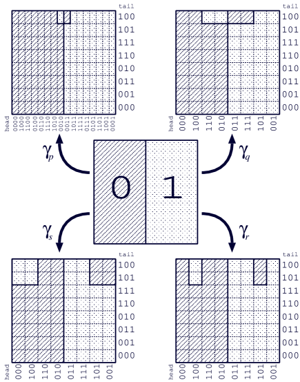
Figure 9. The change of the partition along $\gamma_{p},\gamma_{q},\gamma_{r}$ and $\gamma_{s}$.

Applying the algorithm above to the loop $\gamma_{q}$, we obtain Figure 7 and 8. The interval $[0,1]$ is decomposed into $n=2^{8}$ sub-intervals, and the size of the grid for $\mathbb{C}^{2}$ is $2^{-8}$ in each direction. The lightly and darkly shaded regions in Figure 7 are $N_{0}^{0}$ and $N_{0}^{1}$. Similarly, Figure 8 illustrates $N_{1}^{0}$ and $N_{1}^{1}$. Notice that two partitions differ only in four blocks on the left hand side: two blocks of each of $N_{0}^{0}$ and $N_{0}^{1}$ are interchanged. Using rigorous interval arithmetic, these blocks are identified as blocks corresponding to the symbol sequences $10.100$ and $11.100$ where the dot separates the head and the tail of a sequence. By the head of $s=(s_{i})_{i\in\mathbb{Z}}$ we mean the sequence $\{\dots s_{-3}s_{-2}s_{-1}s_{0}\}$ and by the tail $\{s_{1}s_{2}s_{3}\dots\}$.

We execute the same computation also for loops $\gamma_{p}$, $\gamma_{r}$ and $\gamma_{s}$. This yields Figure 9, which shows a schematic picture of the change along these loops. Notice that “head” and “tail” labels in the figure indicates the symbol coding according to the initial partition $N_{0}^{0}$ and $N_{0}^{1}$, illustrated in the central square.

Now, we can compute the image of $\gamma=\gamma_{p}$ (or $\gamma_{q}$, $\gamma_{r}$, $\gamma_{s}$) by $\rho$ as follows: Choose a symbol sequence $s=(s_{i})_{i\in\mathbb{Z}}\in\Sigma_{2}$. Then $z:=h_{0}(s)$ is located in the central square of Figure 9. By definition, $\rho(\gamma_{p})(s)$ is the symbolic coding of the same point $z$, but with respect to the partition on the top left corner of Figure 9. Since two partitions differ only on blocks $0010.100$ and $0011.100$, it follows that $(\rho(\gamma(s)))_{i}\neq s_{i}$ if and only if $H_{\gamma(0)}^{i}(z)$ is contained in these bocks. Namely,

$$(\rho(\gamma(s)))_{i}=\begin{cases}0&\text{ if }s_{i-3}s_{i-2}s_{i-1}s_{i}s_{i+1}s_{i+2}s_{i+3}=0011100\\ 1&\text{ if }s_{i-3}s_{i-2}s_{i-1}s_{i}s_{i+1}s_{i+2}s_{i+3}=0010100\\ s_{i}&otherwise.\end{cases}$$

Similarly we can compute $\rho(\gamma_{q})$, $\rho(\gamma_{r})$ and $\rho(\gamma_{s})$. This proves Proposition 7.

Counting Periodic Orbits

In this appendix, we prove Theorem 1 directly from Corollary 6, without any monodromy argument. Instead of using Theorem 3, we show that the number of periodic points in $K_{a,c}^{\mathbb{R}}$ is different from that of a full horseshoe. Specifically, we claim that the number of points in $\operatorname{Fix}(H_{a,c}^{n})\cap\mathbb{R}^{2}$ is exactly as in Figure 10.

	$\quad\mathrm{DN}\quad$	$L_{p}\cap\mathbb{R}^{2}$	$L_{q}\cap\mathbb{R}^{2}$	$L_{r}\cap\mathbb{R}^{2}$	$L_{s}\cap\mathbb{R}^{2}$	$\ \mathrm{EMP}\$
$n=3$	8	8	8	2	2	0
$n=4$	16	16	16	16	8	0
$n=5$	32	22	22	22	12	0
$n=6$	64	52	40	52	28	0
$n=7$	128	114	72	72	44	0

Figure 10. The number of points in $\operatorname{Fix}(H_{a,c}^{n})\cap\mathbb{R}^{2}$.

We use the Conley index theory to prove the claim. The reader not familiar with the Conley index may consult [17, 19].

Assume $(a,c)$ is in one of $I_{p}$, $I_{q}$, $I_{r}$ or $I_{s}$. We remark that the uniform hyperbolicity of $K_{a,c}^{\mathbb{R}}$ implies that the number of real periodic points is constant on these intervals.

First we compute a lower bound for the number of periodic points. We begin with finding periodic points numerically. Since periodic points are of saddle type and hence are numerically unstable, we apply the subdivision algorithm [11] to find them. For each periodic orbit found numerically, we then construct a cubical index pair [17]. The existence of a periodic point in this index pair is then proved by the following Conley index version of Lefschetz fixed point theorem.

Theorem 12 ([17, Theorem 10.102]).

Let $(P_{1},P_{0})$ be an index pair for $f$ and $f_{P*}$ the homology index map induced by $f$. If $\sum_{k}(-1)^{k}\operatorname{tr\,}f^{n}_{P*k}\neq 0$ then $\operatorname{Inv}(\operatorname{cl\,}(P_{1}\setminus P_{0}),f)$ contains a fixed point of $f^{n}$.

This theorem assures that there exists at least one periodic orbit in each index pair, and therefore we obtain a lower bound for the number of points in $\operatorname{Fix}(H_{a,c}^{n})\cap\mathbb{R}^{2}$.

To compute an upper bound, we have two methods.

One is to prove the uniqueness of the periodic orbit in each index pair. As long as the size of the grid used in the subdivision algorithm was fine enough, we can expect that each index pair isolates exactly one periodic orbit of period $n$. Since periodic points are hyperbolic, uniqueness can be achieved by a Hartman-Grobman type theorem [2, Proposition 4.1].

The other one is to use the fact that the number of fixed points of $H_{a,c}^{n}:\mathbb{C}^{2}\to\mathbb{C}^{2}$ is independent of the parameter, in fact it is $2^{n}$, counted with multiplicity [13, Theorem 3.1]. In our case, the uniform hyperbolicity implies that the multiplicity is always $1$ and hence there are exactly $2^{n}$ distinct points in $\operatorname{Fix}(H_{a,c}^{n})$. Therefore, if we find $k$ distinct fixed points of $H_{a,c}^{n}$ outside $\mathbb{R}^{2}$, then the cardinality of $\operatorname{Fix}(H_{a,c}^{n})\cap\mathbb{R}^{2}$ must be less than or equal to $2^{n}-k$. Again, we can apply Theorem 12 to establish the existence of fixed points in $\mathbb{C}^{2}\setminus\mathbb{R}^{2}$. This gives an upper bound.

For all cases shown in Figure 10, the lower and upper bounds obtained by methods above coincide. Thus our claim follows.

References

- [1] Z. Arai, On Hyperbolic Plateaus of the Hénon map, to appear in Experimental Mathematics.
- [2] Z. Arai and K. Mischaikow, Rigorous computations of homoclinic tangencies, SIAM Journal on Applied Dynamical Systems 5 (2006), 280–292.
- [3] E. Bedford, M. Lyubich and J. Smillie, Polynomial diffeomorphisms of . IV: The measure of maximal entropy and laminar currents, Invent. math. 112 (1993), 77–125.
- [4] E. Bedford and J. Smillie, Polynomial diffeomorphisms of : currents, equilibrium measure and hyperbolicity, Invent. math. 103 (1991), 69–99.
- [5] E. Bedford and J. Smillie, The Hénon family: The complex horseshoe locus and real parameter values, Contemp. Math. 396 (2006), 21–36.
- [6] P. Blanchard, R. L. Devaney and L. Keen, The dynamics of complex polynomials and automorphisms of the shift, Invent. Math. 104 (1991), 545–580.
- [7] M. Boyle, D. Lind and D. Rudolph, The automorphism group of a shift of finite type, T͡rans. Amer. Math. Soc. 306 (1988), 71–114.
- [8] R. C. Churchill, J. Franke and J. Selgrade, A geometric criterion for hyperbolicity of flows, Proc. Amer. Math. Soc. 62 (1977), 137–143.
- [9] P. Cvitanović, Periodic orbits as the skeleton of classical and quantum chaos, Physica D 51 (1991), 138–151.
- [10] M. J. Davis, R. S. MacKay and A. Sannami, Markov shifts in the Hénon family, Physica D 52 (1991), 171–178.
- [11] M. Dellnitz and O. Junge, Set oriented numerical methods for dynamical systems, Handbook of dynamical systems II, North-Holland, 2002, 221–264.
- [12] R. Devaney and Z. Nitecki, Shift automorphisms in the Hénon mapping, Commun. Math. Phys. 67 (1979), 137–146.
- [13] S. Friedland and J. Milnor, Dynamical properties of plane polynomial automorphisms, Ergodic Theory Dynam. Systems 9 (1989), 67–99.
- [14] G. A. Hedlund, Endomorphisms and automorphisms of the shift dynamical system, Mathematical Systems Theory 3 (1969), 320–375.
- [15] S. L. Hruska, A numerical method for constructing the hyperbolic structure of complex H’enon mappings, Found. Comput. Math. 6 (2006), 427–455.
- [16] S. L. Hruska, Rigorous numerical models for the dynamics of complex H’enon mappings on their chain recurrent sets, Discrete Contin. Dyn. Syst. 15 (2006), 529–558.
- [17] T. Kaczynski, K. Mischaikow and M. Mrozek, Computational Homology, Applied Mathematical Sciences, 157, Springer-Verlag, 2004.
- [18] B. P. Kitchens, Symbolic Dynamics, Springer-Verlag, 1998.
- [19] K. Mischaikow and M. Mrozek, The Conley index theory, Handbook of Dynamical Systems II, North-Holland, 2002, 393–460.
- [20] S. Morosawa, Y. Nishimura, M. Taniguchi and T. Ueda, Holomorphic Dynamics, Cambridge University Press, 2000.
- [21] R. J. Sacker and G. R. Sell, Existence of dichotomies and invariant splitting for linear differential systems I, J. Differential Equations 27 (1974) 429–458.
- [22] M. Shub, Global stability of dynamical systems, Springer-Verlarg, New York, 1987.