Spin dephasing due to a random Berry phase

Abstract

We investigate relaxation and dephasing of an electron spin confined in a semiconductor quantum dot and subject to spin-orbit coupling. Even in vanishing magnetic field, $\bm{B}=0$, slow noise coupling to the electron’s orbital degree of freedom leads to dephasing of the spin due to a random, in general non-Abelian Berry phase acquired by the spin. For illustration we first present a simple quasiclassical description, then consider a model with 2 orbital states only, and finally present a perturbative quantum treatment appropriate for an electron in a realistic (roughly parabolic, not too strongly confining) quantum dot. We further compare the effect of different sources of noise. While at large magnetic fields phonons dominate the relaxation processes, at low fields electron-hole excitations and possibly $1/f$ noise may dominate.

, , , and

1 Introduction

The demonstrations of coherent single-electron spin control and measurement [1, 2, 3] in semiconductor quantum dots have opened exciting perspectives for solid state quantum information processing with spin qubits [4]. More recent work [5, 6, 7, 8] has revealed further potential of spin coherence, which greatly extends the possibilities of next-generation spintronic devices. The key behind these emerging technologies is the long spin coherence time in semiconductor materials. Spins, unlike orbital electron degrees of freedom, do not couple directly to the various sources of electric noise present in typical solid-state environments.

Most of the traditional techniques for addressing and manipulating spins in semiconductors have revolved around some form of electron spin resonance (ESR), be it through external magnetic fields [3] or effective internal ac fields based on the spin-orbit interaction. Indeed, spin-orbit interaction has been proposed theoretically as a way of coherently controlling the spin of confined electrons purely by electrical means [9, 10, 11, 12, 13], and important experimental progress has been made in this direction [14, 15]. By the same token, it has long been understood [16, 17] that spin-orbit interaction is one of the main mechanisms by which electron spins decay and lose coherence in semiconductor heterostructures [18, 19, 20, 21].

As we will discuss in this paper, in the particular case of an electron confined in a quantum dot, a time-dependent (fluctuating or controlled) electric field introduces via the spin-orbit coupling a non-Abelian geometric phase (a generalization of Berry phases) into the spin evolution. This connection between spin-orbit interaction and geometric phases has been noted previously in the context of perturbative analysis of the spin decay of trapped electrons [22]. A similar connection had been discussed for free electrons in the presence of disorder scattering [23].

The geometric character of spin evolution under electric fields has striking consequences both for spin-orbit mediated spin relaxation and decoherence as well as for coherent spin manipulation strategies. Geometric spin evolution under controlled gating is potentially robust, since it is not affected by gate timing errors and certain control voltage inaccuracies. In the case of spin decay, the non-Abelian character of the spin precession under a noisy electric environment results in a saturation of spin relaxation rates at low magnetic fields [16] through a fourth order (in the spin-bath coupling) process previously overlooked in the literature [19, 24, 25]. This spin decay mechanism, which can be called geometric dephasing, requires two independent noise sources coupled to two non-commuting components of the electron spin, whereby the non-Abelian properties of the SU(2) group become relevant. To second order in the spin-bath coupling we also note that a different source of fluctuations other that piezoelectric phonons, namely electron-hole excitations in the metallic environment (ohmic fluctuations), dominate the spin relaxation at low magnetic fields. The reason is the higher density of ohmic fluctuations at low energies as compared to phonons.

The present paper is organized as follows. In Sec. 2 we will present qualitatively the main concepts and consequences of the geometric character of the electrically induced spin precession in leading order in the ratio between dot size to spin-orbit length, $x_{0}/l_{\mathrm{so}}$. In Sec. 3 we consider a model system based on only two orbital states of an electron with spin. This model helps to understand the geometrical evolution of the spin. In Sec. 4 we will perturbatively derive the effective Hamiltonian for an electron in a quantum dot under a fluctuating electric field taking into account all orbital states. This will allow us to analyze the spin relaxation and dephasing under realistic conditions.

2 Geometric spin precession of a strongly confined electron

Electric fields applied to a quantum dot structure induce displacements (and possibly deformations) in the confining potential. In the presence of spin-orbit interaction this will lead to a peculiar geometric evolution of the spin state of the confined electron with important consequences for the relaxation and manipulation of the spin. We will approach the problem by first considering the spin precession due to a geometric phase acquired by the spin of a strongly confined electron, when it is adiabatically transported along a given trajectory in a 2DEG in the presence of spin-orbit coupling.

In semiconductor 2D heterostructures the spin-orbit coupling takes the form ($\hbar=1$ throughout this work)

$$\mathcal{H}_{\mathrm{so}} = \alpha\left(\hat{p}_{y}\hat{\sigma}_{x}-\hat{p}_{x}\hat{\sigma}_{y}\right)+\beta\left(\hat{p}_{y}\hat{\sigma}_{y}-\hat{p}_{x}\hat{\sigma}_{x}\right)$$ (1)

$$= \frac{1}{m}\hat{\bm{p}}\bm{\lambda}^{-1}_{\mathrm{so}}\hat{\bm{\sigma}}\,.$$

Here $\hat{\bm{\sigma}}/2$ and $\hat{\bm{p}}$ are the spin and momentum operators, while $\alpha$ and $\beta$ are the Rashba and linear Dresselhaus couplings, which can be lumped into the spin-orbit tensor

$$\bm{\lambda}_{\mathrm{so}}^{-1}\equiv m\left(\begin{array}[]{cc}-\beta&-\alpha\\ \alpha&\beta\end{array}\right).$$ (4)

It sets the scale for the spin-orbit length $l_{\mathrm{so}}\equiv\sqrt{|\det\bm{\lambda}_{\mathrm{so}}|}=\left(m\sqrt{|\alpha^{2}-\beta^{2}|}\right)^{-1}$. The effective strength of the spin-orbit effects in a quantum dot of size $x_{0}$ is in general proportional to some power of the ratio $x_{0}/l_{\mathrm{so}}$. In typical GaAs/AlGaAs semiconductor heterostructures $l_{\mathrm{so}}\sim 1-5\mathrm{\mu m}$, while $x_{0}\sim 30-100\mathrm{nm}$ so that this ratio is usually quite small, of the order of $0.02$. Other materials, such as InAs, have a much stronger spin-orbit length, in the $l_{\mathrm{so}}\sim 100\mathrm{nm}$ range.

By classical intuition we can anticipate the main effect. We consider an electron in a very strong confinement, forced to move along a path $\mathcal{C}$ with trajectory $\bm{R}_{\mathcal{C}}(t)$. Eq. (1) suggests that the spin-orbit coupling makes the spin precess under an effective magnetic field $\bm{B}_{\mathrm{so}}=\frac{1}{m}\hat{\bm{p}}\bm{\lambda}_{\mathrm{so}}^{-1}$, which couples to the spin similar to a Zeeman term except that the field depends on the electron’s momentum. It raises the question as to what ’value’ one should use for operator $\hat{\bm{p}}$. For a strongly confining potential it turns out that we can simply substitute $\hat{\bm{p}}\rightarrow m{\dot{\bm{R}}}_{\mathcal{C}}$. Hence

$$\bm{B}_{\mathrm{so}}={\dot{\bm{R}}}_{\mathcal{C}}\bm{\lambda}_{\mathrm{so}}^{-1}$$ (5)

From this we derive a spin precession governed by the following SU(2) operator

$$U_{\mathrm{ad}}(t) = T\exp\left(-i\int_{0}^{t}dt\,\bm{B}_{\mathrm{so}}\cdot\hat{\bm{\sigma}}\right)$$ (6)

$$= P\exp\left(-i\int_{\mathcal{C}}d\bm{R}_{\mathcal{C}}\,\bm{\lambda}_{\mathrm{so}}^{-1}\hat{\bm{\sigma}}\right)$$

Here $T$ and $P$ stand for time- and path-ordering operators, respectively. The label ‘adiabatic’ in $U_{\mathrm{ad}}$ refers to the constraint of slow paths, $|{\dot{\bm{R}}}_{\mathcal{C}}|\ll x_{0}\omega_{0}$, typically assumed in most works on Berry phases [27]. As is apparent from Eq. (6), due the peculiar dependence of $\bm{B}_{\mathrm{so}}$ on the velocity ${\dot{\bm{R}}}_{\mathcal{C}}$, the total “geometric spin precession” for propagation along a given path $\mathcal{C}$ depends only on the geometry of $\mathcal{C}$ itself, not on the time dependence of ${\bm{R}}_{\mathcal{C}}$.

Another line of arguments leading to this result was pointed out in Ref. [28]. It is based on the observation that $H_{\mathrm{so}}$ can be diagonalized to first order in $x_{0}/l_{\mathrm{so}}$ by a canonical transformation $\exp{\left(-i\hat{\bm{r}}\bm{\lambda}_{\mathrm{so}}^{-1}\hat{\bm{\sigma}}\right)}$, which in turn implies that in a small dot the effect of spin-orbit coupling moving along a given path can be gauged away by a path-dependent gauge transformation $U_{\mathrm{ad}}$ that rotates the spin just as in Eq. (6).

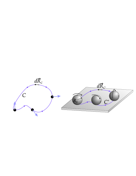
Figure 1: The geometric precession due to spin orbit interaction for an electron adiabatically transported along a path in a 2DEG (left) is equivalent to the changing orientation of a sphere rolling on a plane along a path (right) which is related by a simple transformation to the electron’s path.

The evolution operator $U_{\mathrm{ad}}$ is a group element in SU(2). However, it can also be mapped onto a SO(3) rotation of a 3D solid, since both groups are isomorphic up to a sign. The natural question arises, what is the 3D rotation corresponding to $U_{\mathrm{ad}}$ for a given path? Is there an intuitive visualization that tells us how the spin is rotated as the containing quantum dot is moved? Remarkably, the SO(3) isomorphic form of $U_{\mathrm{ad}}$ (changing the SU(2) generators $\hat{\bm{\sigma}}/2$ by the SO(3) equivalent $\hat{\bm{A}}$) has a very similar form to the operator that gives the orientation of a sphere of radius $R_{0}$ that rolls on a plane without slipping or spinning along a path $\mathcal{C^{\prime}}$ parametrized by $\bm{R}_{\mathcal{C^{\prime}}}(t)$,

$$U_{\mathrm{sph}} = P\exp\left(-i\int_{C^{\prime}}d\bm{R}_{\mathcal{C^{\prime}}}\,\bm{\lambda}_{\mathrm{sph}}^{-1}\hat{\bm{A}}\right)$$ (7)

$$\bm{\lambda}_{\mathrm{sph}}^{-1} = \frac{1}{R_{0}}\left(\begin{array}[]{cc}0&1\\ -1&0\end{array}\right)$$ (10)

This picture of the geometric spin-precession in terms of a rolling sphere is illustrated in Fig. 1. The radius of the sphere is fixed by the spin-orbit length, $R_{0}=l_{\mathrm{so}}/2$. If only Rashba coupling is present there is nothing more to this mapping, since in such case $\bm{\lambda}_{\mathrm{sph}}\propto\bm{\lambda}_{\mathrm{so}}$. However, if Dresselhaus coupling is also present the paths $C$ and $C^{\prime}$ are not exactly the same, but are related by a simple 2D rotation and scaling transformation $\bm{R}_{\mathcal{C^{\prime}}}(t)\bm{\lambda}_{\mathrm{sph}}^{-1}=2\bm{R}_{\mathcal{C}}(t)\bm{\lambda}_{\mathrm{so}}^{-1}$.

This geometrical picture makes it clear that transporting the spin along a sufficiently long straight path $\mathcal{C}$ in a certain direction in the 2DEG will flip the pseudospin. In the case of the sphere moving along a straight path $\mathcal{C^{\prime}}$ the distance needed for a specific rotation does not depend on the direction, but for a spin rotation, due to the nontrivial relation between $\mathcal{C}$ and $\mathcal{C^{\prime}}$ when both Rashba and Dresselhaus couplings are present, the required distance is non-isotropic in a 2DEG. In the direction $[110]$ the spin-flip distance can be strongly enhanced. This non-isotropic property is represented in the Fig. 2 for different ratios of $\beta/\alpha$. In average, the distance that must be covered to induce a pseudospin flip is $\pi l_{\mathrm{so}}/2$, but the variation as a function of the direction can be large whenever $\alpha$ approaches $\beta$.

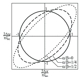
Figure 2: The length of a straight path transport of a small dot required to perform a pseudospin flip as a function of the angle of the path. The three ellipses correspond to different ratios $\beta/\alpha$ but the same value of $l_{\mathrm{so}}$. Dotted ellipse: $\beta/\alpha=1/2$; dashed ellipse: $\beta/\alpha=1/4$, solid ellipse: $\beta/\alpha=0$. The area of the ellipses remains constant and equal to $\pi l_{\mathrm{so}}^{2}$.

3 Two orbital states with spin

3.1 The model

Before analyzing the dynamics of an electron spin in a typical quantum dot we consider a model system with merely two orbital levels, $|0\rangle$ and $|1\rangle$, which are occupied by a single electron with spin-1/2. This model is not valid to describe electrons confined in (near) parabolic quantum dots, where all orbital level are important. Yet, it allows us to get a feeling for the geometric phases acquired by the pseudo-spin states.

The Hilbert space of the model system is spanned by the four states $|0,\uparrow\rangle$, $|0,\downarrow\rangle$, $|1,\uparrow\rangle$, $|1,\downarrow\rangle$. We introduce two sets of Pauli matrices: $\hat{\tau}_{\alpha}$ for orbital degrees of freedom and $\hat{\sigma}_{\alpha}$ for the spin. Thus, for example, $\hat{\tau}_{x}|0\rangle=|1\rangle$, while $\hat{\sigma}_{x}|\uparrow\rangle=|\downarrow\rangle$. In the presence of spin-orbit interaction the Hamiltonian of the model system reads

$$H_{\rm dot}=-\frac{1}{2}\,\epsilon\hat{\tau}_{z}-\frac{1}{2}\,\hat{\tau}_{y}\,\bm{b}\cdot\hat{\bm{\sigma}}\ ,$$ (11)

where $\epsilon$ is the orbital level splitting, while the vector $\bm{b}$ characterizes the Rashba and Dresselhaus spin-orbit coupling. Choosing real orbital wave functions one can easily check that this is the most general form of the spin-orbit coupling allowed by time-reversal symmetry.

Next we introduce the noise which is assumed to couple to the orbital degree of freedom. The general form of coupling is

$$H_{\rm int}=-\frac{1}{2}\,\hat{\tau}_{z}\,\hat{Z}-\frac{1}{2}\,\tau_{x}\,\hat{X}\ ,$$ (12)

where in general $\hat{Z}$ and $\hat{X}$ are quantum fields of a bath governed by the Hamiltonian $H_{\rm bath}$.

For slow noise, i.e. for noise with power spectrum with much weight at low frequencies, instead of considering the coupled quantum dynamics of the dot and the bath, it is sufficient to treat $\hat{Z}$ and $\hat{X}$ as classical stochastic fields, independent of each other. Thus, for transparency, we shall consider the dynamics of the dot subject to the external random fields $Z(t)$ and $X(t)$ and, then, average over realizations of these fields.

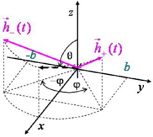
Figure 3: Pseudo-magnetic fields $\bm{h}_{\pm}$.

The resulting total Hamiltonian

$$H_{\rm dot}=-\frac{1}{2}\,\epsilon\hat{\tau}_{z}-\frac{1}{2}\,\hat{\tau}_{y}\,\bm{b}\cdot\hat{\bm{\sigma}}-\frac{1}{2}\,Z(t)\,\hat{\tau}_{z}-\frac{1}{2}\,X(t)\,\hat{\tau}_{x}\ .$$ (13)

shows that the direction of the vector $\bm{b}$ is the natural quantization axis for the spin in our problem. Introducing the corresponding spin basis states $|+\rangle_{\bm{b}}$ and $|-\rangle_{\bm{b}}$ we see that the problem factorizes into two subspaces: $|\Psi_{\rm orbital}\rangle|+\rangle_{\bm{b}}$ and $|\Psi_{\rm orbital}\rangle|-\rangle_{\bm{b}}$. Within each of the two subspaces $(\pm)$ the dynamics is governed by the Hamiltonian

$$H_{\pm} = -\frac{1}{2}\,\epsilon\hat{\tau}_{z}\mp\frac{1}{2}\,b\,\hat{\tau}_{y}-\frac{1}{2}\,Z(t)\,\hat{\tau}_{z}-\frac{1}{2}\,X(t)\,\hat{\tau}_{x}$$ (14)

$$= -\frac{1}{2}\,\bm{h}_{\pm}(t)\hat{\bm{\tau}},$$

where $b\equiv|\bm{b}|$. We have introduced the pseudo-magnetic fields $\bm{h}_{\pm}$ acting on the orbital “pseudo-spin”. These fields are illustrated in Fig. 3. The fields $\bm{h}_{\pm}$ differ only in their $y$-component, $h_{\pm,y}=\pm b$. Therefore we obtain $|\bm{h}_{+}|=|\bm{h}_{-}|$ and – consistent with Kramers’ theorem – we find that the energies of the ground states in the two subspaces, $|g_{+}\rangle|+\rangle_{\bm{b}}$ and $|g_{-}\rangle|-\rangle_{\bm{b}}$, coincide, $E_{g,+}=E_{g,-}=-(1/2)|\bm{h}_{+}|$.

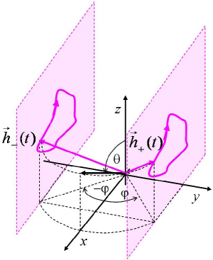
Figure 4: Closed contours traversed by the pseudo-magnetic fields $\bm{h}_{\pm}$.

3.2 Random Berry phase in fluctuating fields

Next we study what happens when the fields $Z(t)$ and $X(t)$ vary in time. In particular, we assume that they traverse slowly a closed contour in the $X-Z$ plane, as illustrated in Fig. 4. Then the pseudo-spin orbital eigenstates states follow their respective pseudo-fields. In addition to the dynamical phase each state acquires a Berry phase. As one can see from Fig. 4, the Berry phases acquired by the two ground states from the subspaces ”+” and ”-” are opposite in sign

$$\Phi_{\pm}=\pm\frac{1}{2}\int d\varphi\cos\theta\ ,$$ (15)

where the angles $\varphi$ and $\theta$ are introduced in Figs. 3 and 4. Since the dynamical phases for the two ground states are the same, the relative phase acquired between the two is

$$\Delta\Phi=\Phi_{+}-\Phi_{-}=\int d\varphi\cos\theta\ .$$ (16)

If we express the angles $\varphi$ and $\theta$ in terms of the fields $X$ and $Z$ and expand assuming $X,Z\ll\epsilon,b$, we find after some algebra

$$\Delta\Phi=\int dt\,\frac{b}{(\epsilon^{2}+b^{2})^{3/2}}\,Z(t)\dot{X}(t)+...\ .$$ (17)

The dots in this relation denote contributions which vanish for closed contours and, as can be shown, do not cause dephasing.

Several notes are in order. Since the evolution of the pseudospin is described here by a single phase $\Delta\Phi$, rotations due to two different loops in the $X-Z$ plane commute. Thus we obtain an Abelian Berry phase. Indeed, as we have seen, the subspaces $+$ and $-$ do not mix. If, initially, we had a superposition $\alpha|g_{+}\rangle|+\rangle_{\bm{b}}+\beta|g_{-}\rangle|-\rangle_{\bm{b}}$, the absolute values $|\alpha|$ and $|\beta|$ are conserved and only the relative phase changes due to the adiabatic evolution.

Treating the quantity $Z(t)\dot{X}(t)$ as a Gaussian stochastic field we obtain the dephasing rate as [29]

$$\Gamma_{\varphi}=\frac{1}{2}\,\frac{b^{2}}{(\epsilon^{2}+b^{2})^{3}}\,S_{Z\dot{X}}(\omega=0)\ ,$$ (18)

where $S_{Z\dot{X}}$ is the spectral density of $Z\dot{X}$. We estimate this quantity as

$$S_{Z\dot{X}}(\omega=0)\sim 2\int\limits_{0}^{T}d\omega\,\omega^{2}S_{X}(\omega)S_{Z}(\omega)\ ,$$ (19)

where the limitation of the integration by the temperature can be justified by noting that any field can be treated classically only at frequencies lower than temperature. A fully quantum mechanical analysis confirms this assertion.

4 Electron spin in a quantum dot

4.1 Effective Hamiltonian

Lifting the restriction to two orbital states, we now consider the full problem of a single electron confined to a lateral quantum dot by the potential $V(\hat{\mathbf{r}})$ in the presence of a magnetic field $\vec{B}$. To be specific, we assume the field to be oriented parallel to the plane of the dot, but our procedure can be generalized to arbitrary directions [30]. The static part of the Hamiltonian then reads

$$H_{\rm 0}=\frac{\mathbf{p}^{2}}{2m^{*}}+V(\mathbf{r})-\frac{g\mu_{B}}{2}\vec{B}\cdot\vec{\sigma}+H_{\mathrm{so}}\,.$$ (20)

The magnetic field couples to the electron through a Zeeman term with material specific $g$-factor . The last term, defined in Eq. 1, describes the Dresselhaus ($\beta$) and Rashba spin-orbit couplings ($\alpha$) between the spin $\vec{\sigma}$ of the electron and its momentum [31]. For a dot of size $x_{0}$ the typical energy of the spin-orbit coupling scales as $\sim\max{\alpha,\beta}/x_{0}$, while the level spacing scales as $\omega_{0}\sim 1/(m^{*}x_{0}^{2})$. Therefore, for dots with small level spacing, $\omega_{0}<1\;{\rm K}$, the spin-orbit coupling cannot be treated perturbatively.

Next we account for time-dependent fluctuations of the electromagnetic field, which add a term

$$\delta V(t)=X^{\mu}(t)\;\hat{O}_{\mu}$$ (21)

to the Hamiltonian. (A summation over repeated indices, such as $\mu$, is assumed throughout.) The terms $\hat{O}_{\mu}$ denote independent operators in the Hilbert space of the confined electron (e.g., $x$, $y$, $x^{2},\dots$), while the terms $X^{\mu}(t)$ denote the corresponding fluctuating (in general quantum) fields (e.g., $\delta E_{x}$, $\delta E_{y}$, $\nabla_{x}\delta E_{x}$, …). They may be generated by various environments, such as phonons, localized defects, or electron-hole excitations. Information about their specific properties is contained in the spectral functions, to be specified later. Note that this formulation covers also quadrupolar fluctuations.

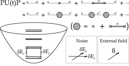
Figure 5: Left: Single electron lateral quantum dot in a magnetic field, which lifts the ground state degeneracy. Virtual transitions to excited states are induced by weak fluctuations of the external fields $\delta E_{x}(t)$, $\delta E_{y}(t)$. Right: Graphical representation of the evolution operator. Virtual transitions to excited states $n$ (wavy lines) are integrated out to yield an effective Hamiltonian within the doublet subspace.

In case of time-reversal symmetry the ground state of the dot is two-fold degenerate. This degeneracy is split in an external magnetic field. If $g\mu_{B}B\ll\omega_{0}$, and as long as the noise is adiabatic with respect to the orbital level splitting, $T\ll\omega_{0}$, the dynamics of the spin remains constrained to these two states. Under these conditions (following the method described in Ref. [32]) we can derive an effective Hamiltonian for the two lowest eigenstates $|\sigma=\pm\rangle$ of $H_{0}$ by expanding the evolution operator $U(t)=\mathrm{T\;exp}\{-i\int_{0}^{t}dt^{\prime}\;{\delta V}_{\rm int}(t^{\prime})\}$ and projecting to the subspace $\{|\sigma\rangle\}$ as sketched in Fig. 5. This results in

$$PU(t)P=1-i\int_{0}^{t}dt_{1}P\delta V_{\rm int}(t_{1})P$$

$$-\int\int_{t_{1}>t_{2}}P\delta V_{\rm int}(t_{1})P\delta V_{\rm int}(t_{2})P$$ (22)

$$-\int\int_{t_{1}>t_{2}}P\delta V_{\rm int}(t_{1})(1-P)\delta V_{\rm int}(t_{2})P+\ldots\;.$$

Here $\delta V_{\rm int}(t)$ denotes the fluctuating part of the Hamiltonian in the interaction representation and $P=\sum_{\sigma}|\sigma\rangle\langle\sigma|$. We separated terms that involve direct transitions between the two lowest states from transitions via excited states. In the spirit of an adiabatic approximation, these latter processes can be integrated out to yield an effective Hamiltonian in the two-dimensional subspace. Technically, this is performed by introducing slow and fast variables, $t\equiv(t_{1}+t_{2})/2$ and $\tau\equiv t_{1}-t_{2}$, in the last term of Eq. (22),

$$\sim\;e^{-it(\epsilon_{\sigma}-\epsilon_{\sigma^{\prime}})-i\tau\left[\frac{1}{2}(\epsilon_{\sigma}+\epsilon_{\sigma^{\prime}})-\epsilon_{n}\right]}\;\delta V_{\sigma n}(t_{1})\delta V_{n\sigma^{\prime}}(t_{2})\;,$$

expanding the interaction potential in $\tau$ as $\delta V(t_{1,2})\approx\delta V(t)\pm\frac{\tau}{2}\;\frac{d}{dt}{\delta V}(t)+\dots$, and integrating with respect to $\tau$. Here $\epsilon_{\sigma}$ and $\epsilon_{n}$ denote the eigenenergies of the lowest doublet and higher eigenstates of $H_{0}$, respectively. In this way the last term in Eq. (22) becomes local in time. Retaining only processes up to 2nd order, we find an effective Hamiltonian within the lowest-energy two-dimensional subspace, characterized by the ‘pseudospin’ Pauli matrices $\tilde{\sigma}_{x,y,z}$,

$$H_{\mathrm{eff}} = -\frac{1}{2}B_{\rm eff}\;{\tilde{\sigma}_{z}}+X^{\mu}\vec{C}^{(1)}_{\mu}\cdot\vec{\tilde{\sigma}}+X^{\mu}X^{\nu}\vec{C}^{(2)}_{\mu\nu}\cdot\vec{\tilde{\sigma}}$$ (23)

$$+ \frac{1}{2}\left(\dot{X}^{\mu}X^{\nu}-X^{\mu}\dot{X}^{\nu}\right)\vec{C}^{(3)}_{\mu\nu}\cdot\vec{\tilde{\sigma}}\;.$$

Due to the spin-orbit coupling, which is not assumed to be weak, eigenstates do not factorize into orbital and spin sectors (hence the term ‘pseudospin’). The static effective field, ${\vec{B}}_{\rm eff}\equiv(\epsilon_{+}-\epsilon_{-})\hat{z}$, accounts for the spin-orbit renormalization of the $g$-factor and defines the $\hat{z}$ direction in the doublet space. The couplings $\vec{C}^{(i)}$, determining the effective fluctuating magnetic fields felt by the pseudospin, are given by

$$\left[\vec{C}^{(1)}_{\mu}\cdot\vec{\tilde{\sigma}}\right]_{\sigma,\sigma^{\prime}}=\hat{O}^{\mu}_{\sigma\sigma^{\prime}}\ ,$$ (24)

$$\left[\vec{C}^{(2)}_{\mu\nu}\cdot\vec{\tilde{\sigma}}\right]_{\sigma,\sigma^{\prime}}=-{\sum_{n}}^{\prime}\frac{\hat{O}^{\mu}_{\sigma n}\hat{O}^{\nu}_{n\sigma^{\prime}}}{\frac{\epsilon_{\sigma}+\epsilon_{\sigma^{\prime}}}{2}-\epsilon_{n}}\ ,$$ (25)

$$\left[\vec{C}^{(3)}_{\mu\nu}\cdot\vec{\tilde{\sigma}}\right]_{\sigma,\sigma^{\prime}}=-i\,{\sum_{n}}^{\prime}\frac{\hat{O}^{\mu}_{\sigma n}\hat{O}^{\nu}_{n\sigma^{\prime}}}{\left(\frac{\epsilon_{\sigma}+\epsilon_{\sigma^{\prime}}}{2}-\epsilon_{n}\right)^{2}}\ .$$ (26)

The summation is restricted to excited states of higher doublets $n\neq\sigma,\sigma^{\prime}$. We do not provide explicit expressions for the eigenenergies $\epsilon_{\sigma}$, $\epsilon_{n}$, matrix elements $\hat{O}^{\mu}_{\sigma\sigma^{\prime}}$, $\hat{O}^{\mu}_{\sigma n}$, or couplings $\vec{C}^{(i)}$, but below we will evaluate them numerically and provide quantitative estimates for a generic model. We further note that both $\vec{C}^{(1)}_{\mu}$ and $\vec{C}^{(3)}_{\mu\nu}$ turn out to be transversal to ${\vec{B}}_{\rm eff}$, therefore contributing only to relaxation, whereas $\vec{C}^{(2)}_{\mu\nu}$ has in general also a parallel component that leads to pure dephasing.

4.2 Geometric phases in $B=0$ case

In time-reversal symmetric situation, (i.e. for $B=0$), the first three terms of Eq. (23) vanish identically [19, 30]. Only the last term survives, and leads to spin dephasing. It has a geometrical origin. To demonstrate this, let us assume that the fluctuating (adiabatic) fields $X_{\mu}$ are classical. We introduce the instantaneous ground states of the Hamiltonian, $|\Phi_{n}(t)\rangle\equiv|\Phi_{n}(X_{\mu}(t))\rangle$ defined through the equation

$$[H_{0}+\delta V(X_{\mu})]|\Phi_{n}(X_{\mu})\rangle=E_{n}(X_{\mu})|\Phi_{n}(X_{\mu})\rangle\;.$$ (27)

Noting that, to lowest order perturbation theory, the two degenerate instantaneous ground states are simply given by $|\Phi_{\sigma}(X_{\mu})\rangle\approx|\sigma\rangle+{\sum_{n}}^{\prime}|n\rangle{\langle n|\delta V|\sigma\rangle}/({\epsilon_{\sigma}-\epsilon_{n}})\;,$ we can rewrite the last term in Eq. (23) in the familiar form

$$H^{\mathrm{eff}}_{\sigma\sigma^{\prime}}(B=0)=-i\langle{\frac{d\Phi_{\sigma}}{dt}|\Phi_{\sigma^{\prime}}}\rangle\;,$$ (28)

which shows clearly that the last term is due to a generalized (possibly non-Abelian) Berry phase [27, 33, 34] acquired in a degenerate 2D subspace. In vanishing magnetic field, Eq. (28) can be shown to hold to all orders of perturbation theory within the adiabatic approximation [30]. If at least two linearly independent fluctuating fields couple to the dot, they can produce a random Berry phase for the system and cause geometric dephasing at $B=0$. When more noise components are present, the Berry phase may become non-Abelian and all components of the spin may decay.

4.3 Relaxation and dephasing times

So far, our treatment has been rather general, applicable for arbitrary noise properties and dot geometries. In its full glory, Eq. (23) describes the motion of the pseudo-spin coupled to three fluctuating “magnetic fields”. In general, the dynamics induced by these non-commuting fields is complicated. To obtain a qualitative understanding of the dynamics we analyze the spin relaxation and pure dephasing times [35], $T_{1}$ and $T_{2}^{*}$ (with $1/T_{2}=1/2T_{1}+1/T_{2}^{*}$). They are defined only for sufficiently strong effective fields, $B_{\rm eff}\gg 1/T_{1},\;1/T^{*}_{2}$. In the limit $B=0$ we evaluate what we call the geometrical dephasing time $T_{\rm geom}$. For the quantitative estimate we consider a parabolic confining potential, $V({\bf r})=\frac{m^{*}\omega_{0}^{2}}{2}|{\bf r}|^{2}$ with level spacing $\omega_{0}$ and typical size $x_{0}=1/\sqrt{\omega_{0}m^{*}}$. Furthermore, we take into account only dipolar fluctuations, $\hat{X}\equiv e\delta E_{x}x_{0}$ and $\hat{Y}\equiv e\delta E_{y}x_{0}$ coupling to the operators ${\hat{O}}_{X}\equiv x/x_{0}$ and ${\hat{O}}_{Y}\equiv y/x_{0}$, respectively. We assume the two components $\hat{X}$ and $\hat{Y}$ to be independent of each other, but to have identical noise spectra, $S_{X}(\omega)=S_{Y}(\omega)=S(\omega)=\pi\varrho(\omega){\rm coth}(\omega/2T)$, with $\varrho(\omega)$ being the spectral function of the bosonic environment (phonons or photons).

The spectral function $\varrho(\omega)$ for phonons can be estimated along the lines of Ref. [19]. For the parameters specified in Ref. [21] we find for piezoelectric phonons in typical GaAs heterostructures at low frequencies, $\varrho_{\rm ph}(\omega)=x_{0}^{2}\;\lambda_{\rm ph}\;\omega^{3}$ with $\lambda_{\rm ph}\approx 4\cdot 10^{-6}{\rm K}^{-2}{\rm nm}^{-2}$. With these parameters we obtain relaxation rates generated by the first term in Eq. (23) that coincide with those of Ref. [21] at not too high values of the field . Similar values are obtained for the parameters of Ref. [36]. For Ohmic fluctuations the spectral function is linear at low frequencies, $\varrho_{\Omega}(\omega)=\lambda_{\Omega}\;\omega$ [37, 38]. The prefactor $\lambda_{\Omega}$ depends on the dimensionless impedance of the circuit, $\lambda_{\Omega}\sim\frac{e^{2}}{h}\;{\rm Re}[Z]$. For typical values of the sheet resistance of the 2-DEG ($10^{2}-10^{3}\Omega/\Box$) we estimate it to be in the range $0.1>\lambda_{\Omega}>0.01$. For $1/f$ noise the power spectrum is $S(\omega)=\lambda_{1/f}/|\omega|$. We will further comment on its strength below.

We first estimate the contributions $T_{1}^{(i)}$ and $T_{2}^{*(i)}$, derived from the three terms ($i=1,2,3$) in Eq. (23), for a non-vanishing in-plane magnetic field, $B_{\rm eff}\gg 1/T_{1},\;1/T^{*}_{2}$. The coupling ${\vec{C}}^{(1)}$ turns out to be perpendicular to ${\vec{B}}_{\rm eff}$ [21], and for low magnetic fields and weak spin-orbit coupling is proportional to $|{\vec{C}}^{(1)}|\sim\frac{B}{x_{0}\omega_{0}^{2}}\;\max\{{\alpha},{\beta}\}$. This fluctuating field therefore contributes to the $T_{1}$ energy relaxation only,

$$\frac{1}{T_{1}^{(1)}}=2\left(|\vec{C}^{(1)}_{X}|^{2}+|\vec{C}^{(1)}_{Y}|^{2}\right)\;S_{X}(B_{\rm eff})\ .$$ (29)

It scales as $1/T_{1}^{(1)}\sim B^{2}\max\{B,T\}$ for Ohmic dissipation and as $\sim B^{4}\max\{B,T\}$ for phonons. As a consequence, for dots with level spacing in the range $\omega_{0}\approx 1\dots 10\;{\rm K}$ Ohmic fluctuations dominate over phonons for low fields with $B<1\dots 3\;{\rm T}$.

The second term, $|{\vec{C}}^{(2)}|\sim\frac{B}{x_{0}^{2}\omega_{0}^{4}}\max\{\alpha^{2},\beta^{2}\}$ gives rise to both relaxation and dephasing.  The two rates are

$$\frac{1}{T_{1}^{(2)}}=4\left(|\vec{C}^{(2,\perp)}_{XX,s}|^{2}+|\vec{C}^{(2,\perp)}_{YY,s}|^{2}+2|\vec{C}^{(2,\perp)}_{XY,s}|^{2}\right)S_{XY}(B_{\rm eff})\;,$$

$$\frac{1}{T_{2}^{*(2)}}=4\left(|\vec{C}^{(2,\parallel)}_{XX,s}|^{2}+|\vec{C}^{(2,\parallel)}_{YY,s}|^{2}+2|\vec{C}^{(2,\parallel)}_{XY,s}|^{2}\right)S_{XY}(0)\;,$$

$$S_{XY}(\omega)=\frac{\pi}{2}\int d\tilde{\omega}\;\frac{\varrho(\frac{\omega+\tilde{\omega}}{2})\varrho(\frac{\omega-\tilde{\omega}}{2})}{1-\cosh(\tilde{\omega}/2T)/\cosh(\omega/2T)}\ ,$$

with $\vec{C}^{(2,\perp/\parallel)}_{\mu\nu,s}$ denoting the symmetrized component of ${\vec{C}}^{(2)}_{\mu\nu}$ perpendicular/parallel to ${\vec{B}}_{\rm eff}$. Thus, for Ohmic dissipation ${1}/{T_{1}^{(2)}}$ vanishes as $\sim B^{2}\max\{B^{3},T^{3}\}$, while for phonons it scales as $\sim B^{2}\max\{B^{7},T^{7}\}$.

$\vec{C}^{(3)}$ is also perpendicular to ${\vec{B}}_{\rm eff}$. Its contribution to the relaxation is

$$\frac{1}{T_{1}^{(3)}} = 2|\vec{C}^{(3)}_{XY,a}|^{2}S_{\dot{X}Y-X\dot{Y}}(B_{\rm eff})\;,$$ (30)

$$S_{\dot{X}Y-X\dot{Y}}(\omega) = \frac{\pi}{2}\int d\tilde{\omega}\;\frac{\tilde{\omega}^{2}\varrho(\frac{\omega+\tilde{\omega}}{2})\varrho(\frac{\omega-\tilde{\omega}}{2})}{1-\cosh(\tilde{\omega}/2T)/\cosh(\omega/2T)}\;,$$

with $\vec{C}^{(3)}_{\mu\nu,a}$ being the anti-symmetrized component of ${\vec{C}}^{(3)}_{\mu\nu}$. Most importantly, with $|{\vec{C}}^{(3)}_{XY}|\sim\frac{1}{x_{0}^{2}\omega_{0}^{4}}\max\{\alpha^{2},\beta^{2}\}$, the rate ${1}/{T_{1}^{(3)}}$ approaches a non-zero value at low fields, $1/T_{1},1/T_{2}^{*}\ll B\ll T$, and scales as $\sim\max\{B^{5},T^{5}\}$ for Ohmic dissipation and $\sim\max\{B^{9},T^{9}\}$ for phonons.

Finally, at $B=0$ the geometric dephasing rate is given by ${1}/{T_{1}^{(3)}}$, extrapolated to zero field

$$\frac{1}{T_{\rm geom}}=2|\vec{C}^{(3)}_{XY,a}|^{2}S_{\dot{X}Y-X\dot{Y}}(\omega\sim 0)\ .$$ (31)

In our example with only two noise components this process dephases only the components of the spin perpendicular to $\vec{C}^{(3)}_{XY}$.

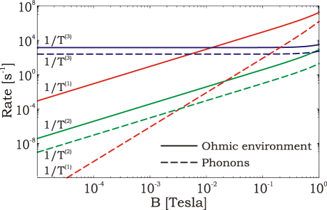
Figure 6: Spin relaxation rates for a GaAs quantum dot with level spacing $\omega_{0}=1{\rm K}$ as function of the Zeeman field. We chose a temperature $T=100\;{\rm mK}$ and Ohmic coupling $\lambda_{\Omega}=0.05$. Below $B^{*}\approx 1\;{\rm T}$ spin relaxation is dominated by coupling to Ohmic fluctuations. For $B<B^{**}\approx 15\;{\rm mT}$ geometrical spin relaxation due to coupling to Ohmic fluctuations dominates. For all $B$ values plotted, the Bloch-Redfield consistency requirement, $B_{\mathrm{eff}}\gg 1/T^{(i)}$, is satisfied.

The relaxation rates corresponding to the different terms in Eq. (23) and various noise sources are shown in Fig. 6. Clearly, for external fields $B<B^{*}\approx 1\dots 3\;{\rm T}$ Ohmic fluctuations provide the leading relaxation mechanism. The crossover field $B^{*}$ is not very sensitive to the specific value of the spectral parameter $\lambda_{\Omega}$ and is independent of the spin-orbit coupling. Below a second crossover field, $B^{**}\approx 15{\rm mT}$, the geometric dephasing induced by Ohmic fluctuations starts to dominate. This second crossover scale is very sensitive to the spin-orbit coupling and temperature, scaling as $B^{**}\sim\max\{\alpha,\beta\}(1/x_{0})(T/\omega_{0})^{2}$. E.g. for a level spacing $\omega_{0}\sim 1{\rm K}$ and temperature $T=100\;{\rm mK}$ ($T=50\;{\rm mK}$) the Berry phase mechanism gives a relaxation time of the order of $700\;{\rm\mu s}$ ($20\;{\rm ms}$). For even lower temperatures or smaller dots with level spacing $\omega_{0}\sim 10{\rm K}$ the $B\to 0$ relaxation time is quickly pushed up to the range of seconds.

Finally, we comment on the effect of $1/f$ noise. In most cases, the non-symmetrized correlators for $1/f$ noise, needed to calculate correlators as $S_{XY}$ or $S_{XX}$, are not known. Yet, for $|\omega|\ll T$ we can provide an estimate $S_{XY}(\omega)\approx\int\limits_{-T}^{T}\frac{d\tilde{\omega}}{2\pi}S_{X}(\omega-\tilde{\omega})S_{Y}(\tilde{\omega})$, and similarly for $S_{\dot{X}Y-X\dot{Y}}$. The $B=0$ geometrical dephasing rate due to the $1/f$ noise can be estimated as $T_{\rm geom}^{-1}\approx|{\vec{C}}^{(3)}_{XY}|^{2}\lambda_{1/f}^{2}(T)\,\omega_{c}$, where $\omega_{c}$ is the upper frequency cut-off for the $1/f$ noise [39]. Accounting for the high-frequency (Ohmic) noise, sometimes observed to be associated with the $1/f$ noise [40, 41, 42, 43], the estimate becomes $T_{\rm geom}^{-1}\approx|{\vec{C}}^{(3)}_{XY}|^{2}\lambda_{1/f}^{2}(T)\,T$. While the $1/f$ noise of background charge fluctuations is well studied in mesoscopic systems, the amplitude of the $1/f$ noise of the electric field in quantum dot systems is yet to be determined. If we assume that this noise is due to two-level systems at the interfaces of the top gate electrodes, we conclude that in the parameter range explored here, the effect of $1/f$ noise is less important than that of Ohmic fluctuations. However, in quantum dots with large level spacings in the low-temperature and low-field regime, these fluctuations could dominate over the effect of Ohmic fluctuations and eventually determine the spin relaxation time.

5 Conclusion

We have shown how spin-orbit interaction in single electron quantum dots induce pseudospin precession within Kramers’ doublets when the quantum dot is adiabatically shifted along a path by electric fields. The precession depends solely on the geometry of the path. We have analyzed the resulting spin decoherence within a model restricted to two orbital states and showed how random geometric phases appear in this model. Then we have studied spin relaxation and dephasing in a quantum dot considering all orbital states. We derived an effective Hamiltonian for the lowest Kramers’ doublet. The geometrical spin precession induced by at least two independent electric fields occurs around non-commuting axis for different paths, so that it becomes a strictly non-Abelian evolution. This has marked consequences for the spin decoherence due to electric field fluctuations. In particular the spin decay rate remains finite as the external magnetic field vanishes. We estimated the rates of relaxation processes due to the coupling to phonons and to the ohmic environment. We find that, owing to the higher excitation density of ohmic fluctuations at low frequencies as compared to phonon fluctuations, the former dominate over the latter in the low field relaxation rates and provide most likely the leading relaxation channel. The underlying spin precession mechanism could also be exploited to electrically manipulate spins, namely if by applying electric fields the electrons can be transported around $\sim\mathrm{\mu m}$-sized loops.

Acknowledgements: We like to thank W.A. Coish and D. Loss for inspiring discussions. G.Z. was supported by the A. von Humboldt Foundation and by Hungarian Grants Nos. NF061726 and T046303.

References

- [1] J. M. Elzerman et al., Single-shot read-out of an individual electron spin in a quantum dot, Nature 430 (2004) 431–435.
- [2] J. R. Petta et al., Coherent manipulation of coupled electron spins in semiconductor quantum dots, Science 309 (2005) 2180–2184.
- [3] F. H. L. Koppens, C. Buizert, K. J. Tielrooij, I. T. Vink, K. C. Nowack, T. Meunier, L. P. Kouwenhoven, L. M. K. Vandersypen, Driven coherent oscillations of a single electron spin in a quantum dot, Nature 442 (2006) 766–771.
- [4] D. Loss, D. P. DiVincenzo, Quantum computation with quantum dots, Phys. Rev. A 57 (1998) 120–126.
- [5] Y. K. Kato, R. C. Myers, A. C. Gossard, D. D. Awschalom, Electron spin interferometry using a semiconductor ring structure, App. Phys. Lett. 86 (2005) 162107.
- [6] E. M. Hankiewicz, G. Vignale, M. E. Flatte, Spin-hall effect in a [110] gaas quantum well, Phys. Rev. Lett. 97 (2006) 266601.
- [7] H. A. Engel, B. I. Halperin, E. I. Rashba, Theory of spin hall conductivity in n-doped gaas, Phys. Rev. Lett. 95 (2005) 166605.
- [8] D. D. Awschalom, M. E. Flatte, Challenges for semiconductor spintronics, Nature Physics 3 (2007) 153–159.
- [9] M. Duckheim, D. Loss, Electric-dipole-induced spin resonance in disordered semiconductors, Nature Physics 2 (2006) 195–199.
- [10] D. Bulaev, D. Loss, Electric dipole spin resonance for heavy holes in quantum dots, Phys. Rev. Lett. 98 (9) (2007) 097202.
- [11] V. N. Golovach, M. Borhani, D. Loss, Electric-dipole-induced spin resonance in quantum dots, Phys. Rev. B 74 (2006) 165319.
- [12] P. Stano, J. Fabian, Control of electron spin and orbital resonance in quantum dots through spin-orbit interactions, cond-mat/0611228.
- [13] J. M. Tang, J. Levy, M. E. Flatte, All-electrical control of single ion spins in a semiconductor, Phys. Rev. Lett. 97 (2006) 106803.
- [14] J. A. H. Stotz, R. Hey, P. V. Santos, K. H. Ploog, Coherent spin transport through dynamic quantum dots, Nature Materials 4 (2005) 585–588.
- [15] Y. Kato, R. C. Myers, A. C. Gossard, D. D. Awschalom, Coherent spin manipulation without magnetic fields in strained semiconductors, Nature 427 (2004) 50–53.
- [16] E. Abrahams, Donor electron spin relaxation in silicon, Phys. Rev. 107 (1957) 491–496.
- [17] M. I. Dyakonov, V. I. Perel, Spin relaxation of conduction electrons in noncentrosymmetric semiconductors, Soviet Physics Solid State,Ussr 13 (1972) 3023–3026.
- [18] A. V. Khaetskii, Y. V. Nazarov, Spin relaxation in semiconductor quantum dots, Phys. Rev. B 61 (2000) 12639–12642.
- [19] A. V. Khaetskii, Y. V. Nazarov, Spin-flip transitions between zeeman sublevels in semiconductor quantum dots, Phys. Rev. B 64 (2001) 125316.
- [20] L. M. Woods, T. L. Reinecke, Y. Lyanda-Geller, Spin relaxation in quantum dots, Phys. Rev. B 66 (2002) 161318.
- [21] V. N. Golovach, A. Khaetskii, D. Loss, Phonon-induced decay of the electron spin in quantum dots, Phys. Rev. Lett. 93 (2004) 016601.
- [22] P. San-Jose, G. Zarand, A. Shnirman, G. Schön, Geometrical spin dephasing in quantum dots, Phys. Rev. Lett. 97 (2006) 076803.
- [23] Y. A. Serebrennikov, Geometric origin of elliott spin decoherence in metals and semiconductors, Phys. Rev. Lett. 93 (2004) 266601.
- [24] P. Stano, J. Fabian, Orbital and spin relaxation in single and coupled quantum dots, Phys. Rev. B 74 (2006) 045320.
- [25] Y. G. Semenov, K. W. Kim, Elastic spin relaxation processes in semiconductor quantum dots, cond-mat/0612333.
- [26] R. S. Whitney, Y. Makhlin, A. Shnirman, Y. Gefen, Geometric nature of the environment-induced berry phase and geometric dephasing, Phys. Rev. Lett. 94 (2005) 070407.
- [27] M. V. Berry, Quantal phase-factors accompanying adiabatic changes, Proc. R. Soc. London A 392 (1984) 45–57.
- [28] W. A. Coish, V. N. Golovach, J. C. Egues, D. Loss, Measurement, control, and decay of quantum-dot spins, Physica Status Solidi B-Basic Solid State Physics 243 (2006) 3658–3672.
- [29] Y. Makhlin, G. Schön, A. Shnirman, New directions in mesoscopic physics (towards nanoscience), in: R. Fazio, V. F. Gantmakher, Y. Imry (Eds.), NATO-ASI Proceedings, Kluwer, Erice (Italy), 2002, pp. 197 – 224, cond-mat/0309049.
- [30] P. San-Jose et al., to be published.
- [31] R. Winkler, Spin-orbit coupling effects in two-dimensional electron and hole systems, Springer Tracts in Modern Physics, 2003.
- [32] C. Hutter, A. Shnirman, Y. Makhlin, G. Schön, Tunable coupling of qubits: nonadiabatic corrections, Europhys. Lett. 74 (2006) 1088.
- [33] F. Wilczek, A. Zee, Appearance of gauge structure in simple dynamical-systems, Phys. Rev. Lett. 52 (1984) 2111–2114.
- [34] C. A. Mead, Molecular kramers degeneracy and non-abelian adiabatic phase-factors, Phys. Rev. Lett. 59 (1987) 161–164.
- [35] F. Bloch, Generalized theory of relaxation, Phys. Rev. 105 (1957) 1206–1222.
- [36] P. Stano, J. Fabian, Theory of phonon-induced spin relaxation in laterally coupled quantum dots, Phys. Rev. Lett. 96 (18) (2006) 186602.
- [37] A. J. Leggett et al., Dynamics of the dissipative 2-state system, Rev. Mod. Phys. 59 (1987) 1–85.
- [38] U. Weiss, Quantum dissipative systems, 2nd Edition, World Scientific, Singapore, 1999.
- [39] G. Ithier et al., Decoherence in a superconducting quantum bit circuit, Phys. Rev. B 72 (2005) 134519.
- [40] O. Astafiev, Y. A. Pashkin, Y. Nakamura, T. Yamamoto, J. S. Tsai, Quantum noise in the josephson charge qubit, Phys. Rev. Lett. 93 (2004) 267007.
- [41] A. Shnirman, G. Schön, I. Martin, Y. Makhlin, Low- and high-frequency noise from coherent two-level systems, Phys. Rev. Lett. 94 (2005) 127002.
- [42] L. Faoro, J. Bergli, B. L. Altshuler, Y. M. Galperin, Models of environment and t-1 relaxation in josephson charge qubits, Phys. Rev. Lett. 95 (2005) 046805.
- [43] O. Astafiev, Y. A. Pashkin, Y. Nakamura, T. Yamamoto, J. S. Tsai, Temperature square dependence of the low frequency 1/f charge noise in the josephson junction qubits, Phys. Rev. Lett. 96 (2006) 137001.