Recursive weighted treelike networks

Abstract

We propose a geometric growth model for weighted scale-free networks, which is controlled by two tunable parameters. We derive exactly the main characteristics of the networks, which are partially determined by the parameters. Analytical results indicate that the resulting networks have power-law distributions of degree, strength, weight and betweenness, a scale-free behavior for degree correlations, logarithmic small average path length and diameter with network size. The obtained properties are in agreement with empirical data observed in many real-life networks, which shows that the presented model may provide valuable insight into the real systems.

1 Introduction

Complex networks AlBa02 ; DoMe02 ; Ne03 ; BoLaMoChHw06 ; BoSaVe07 describe a number of real-life systems in nature and society, such as Internet FaFaFa99 , World Wide Web AlJeBa99 , metabolic networks JeToAlOlBa00 , protein networks in the cell JeMaBaOl01 , worldwide airport networks BaBaPaVe04 ; LiCa04 , co-author networks Ne01a ; Newman01 ; BaJeNeRaScVi02 ; LiWuWaZhDiFa07 and sexual networks LiEdAmStAb01 . Since the publication of the pioneering papers by Watts and Strogatz on small-world networks WaSt98 and Barabási and Albert on scale-free networks BaAl99 , modeling real-life systems has attracted an exceptional amount of attention within the physics community AlBa02 ; DoMe02 ; Ne03 ; BoLaMoChHw06 ; BoSaVe07 .

Up to now, the research on modeling real-life systems has been primarily focused on binary networks, i.e., edges among nodes are either present or absent, represented as binary states. The purely topological structure of binary networks, however, misses some important attributes of real-world networks. Actually, many real networked systems exhibit a large heterogeneity in the capacity and the intensity of the connections, which is far beyond Boolean representation. Examples include strong and weak ties between individuals in social networks Ne01a ; Newman01 ; BaJeNeRaScVi02 ; LiWuWaZhDiFa07 , the varying interactions of the predator-prey in food networks KrFrMaUlTa03 , unequal traffic on the Internet FaFaFa99 or of the passengers in airline networks BaBaPaVe04 ; LiCa04 . These systems can be better described in terms of weighted networks, where the weight on the edge provides a natural way to take into account the connection strength. In the last few years, modeling real systems as weighted complex networks has attracted an exceptional amount of attention.

The first evolving weighted network model was proposed by Yook et al. (YJBT model) YoJeBaTu01 , where the topology and weight are driven by only the network connection based on preferential attachment (PA) rule. In Ref. ZhTrZhHu03 , a generalized version of the YJBT model was presented, which incorporates a random scheme for weight assignments according to both the degree and the fitness of a node. In the YJBT model and its generalization, edge weights are randomly assigned when the edges are created, and remain fixed thereafter. These two models overlook the possible dynamical evolution of weights occurring when new nodes and edges enter the systems. On the other hand, the evolution and reinforcements of interactions is a common characteristic of real-life networks, such as airline networks BaBaPaVe04 ; LiCa04 and scientific collaboration networks Ne01a ; Newman01 ; BaJeNeRaScVi02 ; LiWuWaZhDiFa07 . To better mimic the reality, Barrat, Barthélemy, and Vespignani introduced a model (BBV) for the growth of weighted networks that couples the establishment of new edges and nodes and the weights’ dynamical evolution BaBaVe04a ; BaBaVe04b . The BBV model is based on a weight-driven dynamics AnKr05 and on a weights’ reinforcement mechanism, it is the first weighted network model that yields a scale-free behavior for the weight, strength, and degree distributions. Enlightened by BBV’s remarkable work, various weighted network models have been proposed to simulate or explain the properties found in real systems BoLaMoChHw06 ; BoSaVe07 ; WaWaHuYaQu05 ; WuXuWa05 ; GoKaKi05 ; MuMa06 ; XiWaWa07 ; LiWaFaDiWu06 .

While a lot of models for weighted networks have been presented, most of them are stochastic BoLaMoChHw06 . Stochasticity present in previous models, while according with the major properties of real-life systems, makes it difficult to gain a visual understanding of how do different nodes relate to each other forming complex weighted networks BaRaVi01 . It would therefore of major theoretical interest to build deterministic weighted network models. Deterministic network models allow one to compute analytically their features, which play a significant role, both in terms of explicit results and as a guide to and a test of simulated and approximate methods BaRaVi01 ; DoGoMe02 ; CoFeRa04 ; ZhRoZh07 ; JuKiKa02 ; RaSoMoOlBa02 ; RaBa03 ; AnHeAnSi05 ; DoMa05 ; ZhCoFeRo05 ; ZhRo05 ; Bobe05 ; BeOs79 ; HiBe06 ; CoOzPe00 ; CoSa02 ; ZhRoGo05 ; ZhRoCo05a . So far, the first and the only deterministic weighted network model has been proposed by Dorogovtsev and Mendes (DM) DoMe05 . In the DM model, only the distributions of the edge weight, of node degree and of the node strength are computed, while other characteristics are omitted.

In this paper, we introduce a deterministic model for weighted networks using a recursive construction. The model is controlled by two parameters. We present an exhaustive analysis of many properties of our model, and obtain the analytic solutions for most of the features, including degree distributions, strength distribution, weight distribution, betweenness distribution, degree correlations, average path length, and diameter. The obtained statistical characteristics are equivalent with some random models (including BBV model).

2 The model

The network, controlled by two parameters $m$ and $\delta$, is constructed in a recursive way. We denote the network after $t$ steps by $Q(t)$, $t\geq 0$ (see Fig. 1). Then the network at step $t$ is constructed as follows. For $t=0$, $Q(0)$ is an edge with unit weight connecting two nodes. For $t\geq 1$, $Q(t)$ is obtained from $Q(t-1)$. We add $mw$ ($m$ is positive integer) new nodes for either end of each edge with weight $w$, and connect each of $mw$ new nodes to one end of the edge by new edges of unit weight; moreover, we increase weight $w$ of the edge by $m\delta w$ ($\delta$ is positive integer). In the special case $\delta=0$, it becomes binary networks, where all edges are identical JuKiKa02 ; GhOhGoKaKi04 ; Bobe05 .

Figure 1: Illustration of a deterministically growing network in the case of $m=2$ and $\delta=1$, showing the first three steps of growing process. The bare edges denote the edges of weight 1.

Let us consider the total number of nodes $N_{t}$, the total number of edges $E_{t}$ and the total weight of all edges $W_{t}$ in $Q(t)$. Denote $n_{v}(t)$ as the number of nodes created at step $t$. Note that the addition of each new node leads to only one new edge, so the number of edges generated at step $t$ is $n_{e}(t)=n_{v}(t)$. By construction, for $t\geq 1$, we have

$$n_{v}(t)=2mW_{t-1},$$ (1)

$$E_{t}=E_{t-1}+n_{v}(t),$$ (2)

and

$$W_{t}=W_{t-1}(1+m\delta)+2mW_{t-1}.$$ (3)

On the right-hand side of Eq. (3), the first item is the sum of weigh of the old edges, and the second term describe the total weigh of the new edges generated in step $t$. We can simplify Eq. (3) to yield

$$W_{t}=(1+m\delta+2m)W_{t-1}.$$ (4)

Considering the initial condition $W_{0}=1$, we obtain

$$W_{t}=(1+m\delta+2m)^{t}.$$ (5)

Substituting Eq. (5) into Eq. (1), the number of nodes created at step $t$ ($t\geq 1$) is obtained to be

$$n_{v}(t)=2m(1+m\delta+2m)^{t-1}.$$ (6)

Then the total number of nodes present at step $t$ is

$$N_{t} =\sum_{t_{i}=0}^{t}n_{v}(t_{i})$$

$$=\frac{2}{2+\delta}\,\left[(1+m\delta+2m)^{t}+\delta+1\right].$$ (7)

Combining Eq. (6) with Eq. (2) and considering $E_{0}=1$, it follows that

$$E_{t}=\frac{2}{2+\delta}\,\left[(1+m\delta+2m)^{t}+\delta\right].$$ (8)

Thus for large $t$, the average node degree $\overline{k}_{t}=\frac{2E_{t}}{N_{t}}$ and average edge weight $\overline{w}_{t}=\frac{W_{t}}{E_{t}}$ are approximately equal to $2$ and $\frac{2+\delta}{2}$, respectively.

3 Network properties

Below we will find that the tunable parameters $m$ and $\delta$ control some relevant characteristics of the weighted network $Q(t)$. We focus on the weight distribution, strength distribution, degree distribution, degree correlations, betweenness distribution, average path length, and diameter.

3.1 Weight distribution

Note that all the edges emerging simultaneously have the same weight. Let $w_{e}(t)$ be the weight of edge $e$ at step $t$. Then by construction, we can easily have

$$w_{e}(t)=(1+m\delta)w_{e}(t-1).$$ (9)

If edge $e$ enters the network at step $\tau$, then $w_{e}(\tau)=1$. Thus

$$w_{e}(t)=(1+m\delta)^{t-\tau}.$$ (10)

Therefore, the weight spectrum of the network is discrete. It follows that the weight distribution is given by

$$P(w)=\left\{\begin{array}[]{lc}{\displaystyle{n_{e}(0)\over E_{t}}={\delta+2\over 2[(1+m\delta+2m)^{t}+\delta]}}&\ \hbox{for}\ \tau=0,\\ {\displaystyle{n_{e}(\tau)\over E_{t}}={m(2+\delta)\,(1+m\delta+2m)^{\tau-1}\over(1+m\delta+2m)^{t}+\delta}}&\ \hbox{for}\ \tau\geq 1,\\ 0&\ \hbox{otherwise}\end{array}\right.$$ (11)

and that the cumulative weight distribution Ne03 ; DoGoMe02 is

$$P_{\rm cum}(w) =\sum_{\mu\leq\tau}\frac{n_{e}(\mu)}{E_{t}}$$

$$={(1+m\delta+2m)^{\tau}+\delta\over(1+m\delta+2m)^{t}+\delta}.$$ (12)

Substituting for $\tau$ in this expression using $\tau=t-\frac{\ln w}{\ln(1+m\delta)}$ gives

$$P_{\rm cum}(w) ={(1+m\delta+2m)^{t}w^{-\frac{\ln(1+m\delta+2m)}{\ln(1+m\delta)}}+\delta\over(1+m\delta+2m)^{t}+\delta}$$

$$\approx w^{-\frac{\ln(1+m\delta+2m)}{\ln(1+m\delta)}}\qquad\qquad\hbox{for large $t$}.$$ (13)

So the weight distribution follows a power law with the exponent $\gamma_{w}=1+{\frac{\ln(1+m\delta+2m)}{\ln(1+m\delta)}}$.

3.2 Strength distribution

In a weighted network, a node strength is a natural genearlization of its degree. The strength $s_{i}$ of node $i$ is defined as

$$s_{i}=\sum_{j\in\Omega_{i}}w_{ij}\,,$$ (14)

where $w_{ij}$ denotes the weight of the edge between nodes $i$ and $j$, $\Omega_{i}$ is the set of all the nearest neighbors of $i$. The strength distribution $P(s)$ measures the probability that a randomly selected node has exactly strength $s$.

Let $s_{i}(t)$ be the strength of node $i$ at step $t$. If node $i$ is added to the network at step $t_{i}$, then $s_{i}(t_{i})=1$. Moreover, we introduce the quantity $\Delta s_{i}(t)$, which is defined as the difference between $s_{i}(t)$ and $s_{i}(t-1)$. By construction, we can easily obtain

$$\Delta s_{i}(t) =s_{i}(t)-s_{i}(t-1)$$

$$=m\delta\sum_{j\in\Omega_{i}}w_{ij}+m\sum_{j\in\Omega_{i}}w_{ij}$$

$$=m\delta s_{i}(t-1)+m\,s_{i}(t-1).$$ (15)

Here the first item accounts for the increase of weight of the old edges incident with $i$, which exist at step $t-1$. The second term describe the total weigh of the new edges with unit weight that are generated at step $t$ and connected to node $i$.

From Eq. (3.2), we can derive following recursive relation:

$$s_{i}(t)=(1+m\delta+m)s_{i}(t-1).$$ (16)

Using $s_{i}(t_{i})=1$, we obtain

$$s_{i}(t)=(1+m\delta+m)^{t-t_{i}}.$$ (17)

Since the strength of each node has been obtained explicitly as in Eq. (17), we can get the strength distribution via its cumulative distribution Ne03 ; DoGoMe02 , i.e.

$$P_{\rm cum}(s) =\sum_{\mu\leq t_{i}}\frac{n_{v}(\mu)}{N_{t}}$$

$$={(1+m\delta+2m)^{t_{i}}+\delta+1\over(1+m\delta+2m)^{t}+\delta+1}.$$ (18)

From Eq. (17), we can derive $t_{i}=t-\frac{\ln s}{\ln(1+m\delta+m)}$. Substituting the obtained result of $t_{i}$ into Eq. (3.2) gives

$$P_{\rm cum}(s) = {(1+m\delta+2m)^{t}\,s^{-\frac{\ln(1+m\delta+2m)}{\ln(1+m\delta+m)}}+\delta+1\over(1+m\delta+2m)^{t}+\delta+1}$$ (19)

$$\approx s^{-\frac{\ln(1+m\delta+2m)}{\ln(1+m\delta+m)}}\qquad\qquad\hbox{for large $t$}.$$

Thus, node strength distribution exhibits a power law behavior with the exponent $\gamma_{s}=1+{\frac{\ln(1+m\delta+2m)}{\ln(1+m\delta+m)}}$.

3.3 Degree distribution

The most important property of a node is the degree, which is defined as the number of edges incident with the node. Similar to strength, in our model, all simultaneously emerging nodes have the same degree. Let $k_{i}(t)$ be the degree of node $i$ at step $t$. If node $i$ is added to the graph at step $t_{i}$, then by construction $k_{i}(t_{i})=1$. After that, the degree $k_{i}(t)$ evolves as

$$k_{i}(t)=k_{i}(t-1)+m\,s_{i}(t-1),$$ (20)

where $ms_{i}(t-1)$ is the degree increment $\Delta k_{i}(t)$ of node $i$ at step $t$. Substituting Eq. (17) into Eq. (20), we have

$$\Delta k_{i}(t)=m\,(1+m\delta+m)^{t-1-t_{i}}.$$ (21)

Then the degree $k_{i}(t)$ of node $i$ at time $t$ is

$$k_{i}(t) =k_{i}(t_{i})+\sum_{\eta=t_{i}+1}^{t}{\Delta k_{i}(\eta)}$$

$$=\frac{(m\delta+1+m)^{t-t_{i}}+\delta}{\delta+1}.$$ (22)

Analogously to computation of cumulative strength distribution, one can find the cumulative degree distribution

$$P_{\rm cum}(k) ={(1+m\delta+2m)^{t}\,[(\delta+1)\,k-\delta]^{-\frac{\ln(1+m\delta+2m)}{\ln(1+m\delta+m)}}\over(1+m\delta+2m)^{t}+\delta+1}$$

$$\quad+{\delta+1\over(1+m\delta+2m)^{t}+\delta+1}$$

$$\approx[(\delta+1)\,k]^{-\frac{\ln(1+m\delta+2m)}{\ln(1+m\delta+m)}}\qquad\hbox{for large $t$}.$$ (23)

Thus, the degree distribution is scale-free with the same exponent as $\gamma_{s}$, that is $\gamma_{k}=\gamma_{s}=1+{\frac{\ln(1+m\delta+2m)}{\ln(1+m\delta+m)}}$.

3.4 Betweenness distribution

Betweenness of a node is the accumulated fraction of the total number of shortest paths going through the given node over all node pairs Fr77 ; Newman01 . More precisely, the betweenness of a node $i$ is

$$b_{i}=\sum_{j\neq i\neq k}\frac{\sigma_{jk}(i)}{\sigma_{jk}},$$ (24)

where $\sigma_{jk}$ is the total number of shortest path between node $j$ and $k$, and $\sigma_{jk}(i)$ is the number of shortest path running through node $i$.

Since the considered network here is a tree, for each pair of nodes there is a unique shortest path between them SzMiKe02 ; BoRi04 ; GhOhGoKaKi04 . Thus the betweenness of a node is simply given by the number of distinct shortest paths passing through the node. From Eqs. (21) and (3.3), we can easily derive that for $\alpha<\theta$ the number of nodes with degree $\frac{(m\delta+1+m)^{\alpha}+\delta}{\delta+1}$ which are direct children of a node with degree $\frac{(m\delta+1+m)^{\theta}+\delta}{\delta+1}$ is $m(1+m\delta+m)^{\tau-1-\alpha}$. Then at time $t$, the betweenness of a $\theta$-generation-old node $v$, which is created at step $t-\theta$, denoted as $b_{t}(\theta)$ becomes

$$b_{t}(\theta) =\mathcal{C}_{t}^{\theta}\,\left[N_{t}-\left(\mathcal{C}_{t}^{\theta}+1\right)\right]+\binom{\mathcal{C}_{t}^{\theta}}{2}$$

$$\quad-\sum_{\alpha=1}^{\theta-1}m(1+m\delta+m)^{\tau-1-\alpha}\binom{\mathcal{C}_{t}^{\alpha}+1}{2},$$ (25)

where $\mathcal{C}_{t}^{\theta}$ denotes the total number of descendants of node $v$ at time $t$, where the descendants of a node are its children, its children’s children, and so on. Note that the descendants of node $v$ exclude $v$ itself. The first term in Eq. (3.4) counts shortest paths from descendants of $v$ to other vertices. The second term accounts for the shortest paths between descendants of $v$. The third term describes the shortest paths between descendants of $v$ that do not pass through $v$.

To find $b_{t}(\theta)$, it is necessary to explicitly determine the descendants $\mathcal{C}_{t}^{\theta}$ of node $v$, which is related to that of $v^{\prime}s$ children via GhOhGoKaKi04

$$\mathcal{C}_{t}^{\theta}=\sum_{\alpha=1}^{\theta}m(1+m\delta+m)^{\alpha-1}\left(\mathcal{C}_{t}^{\tau-\alpha}+1\right).$$ (26)

Using $\mathcal{C}_{t}^{0}=0$, we can solve Eq. (26) inductively,

$$\mathcal{C}_{t}^{\theta}=\frac{1}{\delta+2}\left[(m\delta+1+2m)^{\tau}-1\right].$$ (27)

Substituting the result of Eq. (27) and (2) into Eq. (3.4), we have

$$b_{t}(\theta)\simeq\frac{2}{(\delta+2)^{2}}\,(m\delta+1+2m)^{t+\tau}.$$ (28)

Then the cumulative betweenness distribution is

$$P_{\rm cum}(b) =\sum_{\mu\leq t-\tau}\frac{n_{v}(\mu)}{N_{t}}$$

$$={(1+m\delta+2m)^{t-\tau}+\delta+1\over(1+m\delta+2m)^{t}+\delta+1}$$

$$\simeq{(1+m\delta+2m)^{t}\over(1+m\delta+2m)^{t+\tau}}\sim{N_{t}\over b}\sim b^{-1},$$ (29)

which shows that the betweenness distribution exhibits a power law behavior with exponent $\gamma_{b}=2$, the same scaling has been also obtained for the $m=1$ case of the Barabási-Albert (BA) model describing a random scale-free treelike network SzMiKe02 ; BoRi04 .

3.5 Degree correlations

Degree correlation is a particularly interesting subject in the field of network science MsSn02 ; PaVaVe01 ; VapaVe02 ; Newman02 ; Newman03c ; ZhZh07 , because it can give rise to some interesting network structure effects. An interesting quantity related to degree correlations is the average degree of the nearest neighbors for nodes with degree $k$, denoted as $k_{\rm nn}(k)$ PaVaVe01 ; VapaVe02 . When $k_{\rm nn}(k)$ increases with $k$, it means that nodes have a tendency to connect to nodes with a similar or larger degree. In this case the network is defined as assortative Newman02 ; Newman03c . In contrast, if $k_{\rm nn}(k)$ is decreasing with $k$, which implies that nodes of large degree are likely to have near neighbors with small degree, then the network is said to be disassortative. If correlations are absent, $k_{\rm nn}(k)=const$.

We can exactly calculate $k_{\rm nn}$ for the networks using Eq. (3.3) to work out how many links are made at a particular step to nodes with a particular degree. We place emphasis on the particular case of $\delta=0$. Except for the initial two nodes generated at step 0, no nodes born in the same step, which have the same degree, will be linked to each other. All links to nodes with larger degree are made at the creation step, and then links to nodes with smaller degree are made at each subsequent steps. This results in the expression ZhRoZh07 ; DoMa05 for $k=(m+1)^{t-t_{i}}$

$$k_{\rm nn}(k) ={1\over n_{v}(t_{i})k(t_{i},t)}$$

$$\quad\Bigg{(}\sum_{t^{\prime}_{i}=0}^{t^{\prime}_{i}=t_{i}-1}m\cdot n_{v}(t^{\prime}_{i})k(t^{\prime}_{i},t_{i}-1)k(t^{\prime}_{i},t)$$

$$\quad+\sum_{t^{\prime}_{i}=t_{i}+1}^{t^{\prime}_{i}=t}m\cdot n_{v}(t_{i})k(t_{i},t^{\prime}_{i}-1)k(t^{\prime}_{i},t)\Bigg{)},$$ (30)

where $k(t_{i},t)$ represents the degree of a node at step $t$, which was generated at step $t_{i}$. Here the first sum on the right-hand side accounts for the links made to nodes with larger degree (i.e. $t^{\prime}_{i}<t_{i}$) when the node was generated at $t_{i}$. The second sum describes the links made to the current smallest degree nodes at each step $t^{\prime}_{i}>t_{i}$.

Substituting Eqs. (6) and (3.3) into Eq. (3.5), after some algebraic manipulations, Eq. (3.5) is simplified to

$$k_{\rm nn}(k) =\frac{2m+1}{m}\,\left[\frac{(m+1)^{2}}{2m+1}\right]^{t_{i}}$$

$$\quad-\frac{m+1}{m}+\frac{m}{m+1}\,(t-t_{i}).$$ (31)

Thus after the initial step $k_{\rm nn}$ grows linearly with time.

Writing Eq. (3.5) in terms of $k$, it is straightforward to obtain

$$k_{\rm nn}(k) =\frac{2m+1}{m}\,\left[\frac{(m+1)^{2}}{2m+1}\right]^{t}\,k^{-\frac{\ln\left[\frac{(m+1)^{2}}{2m+1}\right]}{\ln(m+1)}}$$

$$\quad-\frac{m+1}{m}+\frac{m}{m+1}\,\frac{\ln k}{\ln(m+1)}.$$ (32)

Therefore, $k_{\rm nn}(k)$ is approximately a power law function of $k$ with negative exponent, which shows that the networks are disassortative. Note that $k_{\rm nn}(k)$ of the Internet exhibit a similar power-law dependence on the degree $k_{\rm nn}(k)\sim k^{-\omega}$, with $\omega=0.5$ PaVaVe01 . Additionally, one can easily check that for other values of $\delta>0$, the networks will again be disassortative with respect to degree because of the lack of connections between nodes with the same degree.

3.6 Average path length

Most real-life systems are small-world, i.e., they have a logarithmic average path length (APL) with the number of their nodes. Here APL means the minimum number of edges connecting a pair of nodes, averaged over all node pairs. For general $m$ and $\delta$, it is not easy to derive a closed formula for the average path length of $Q(t)$. However, for the particular case of $m=1$ and $\delta=0$, the network has a self-similar structure, which allows one to calculate the APL analytically.

For simplicity, we denote the limiting network ($m=1$ and $\delta=0$) after $t$ generations by $Q_{t}$. Then the average path length of $Q_{t}$ is defined to be:

$$\bar{d}_{t}=\frac{D_{t}}{N_{t}(N_{t}-1)/2}\,.$$ (33)

In Eq. (33), $D_{t}$ denotes the sum of the total distances between two nodes over all pairs, that is

$$D_{t}=\sum_{i,j\in Q_{t}}d_{i,j}\,,$$ (34)

where $d_{i,j}$ is the shortest distance between node $i$ and $j$.

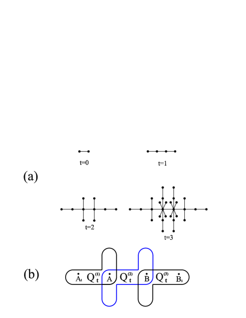
Figure 2: (Color online) (a) The first four steps of binary network growth for the limiting case of $m=1$ and $\delta=0$ are shown. (b) The network after $t+1$ generation, $Q_{t+1}$, can be obtained by joining three copies of generations $t$ (i.e. $Q_{t}^{(1)},Q_{t}^{(2)},Q_{t}^{(3)}$) at the two hub nodes of highest degree, denoted by $A$ and $B$.

We can exactly calculate $\bar{d}_{t}$ according to the self-similar network structure HiBe06 . As shown in Fig. 2, the network $Q_{t+1}$ may be obtained by joining at the hubs (the most connected nodes) three copies of $Q_{t}$, which we label $Q_{t}^{(\alpha)}$, $\alpha=1,2,3$ Bobe05 ; CoRobA05 . Then one can write the sum over all shortest paths $D_{t+1}$ as

$$D_{t+1}=3D_{t}+\Delta_{t}\,,$$ (35)

where $\Delta_{t}$ is the sum over all shortest paths whose endpoints are not in the same $Q_{t}$ branch. The solution of Eq. (35) is

$$D_{t}=3^{t-1}D_{1}+\sum_{\tau=1}^{t-1}3^{t-\tau-1}\Delta_{\tau}\,.$$ (36)

The paths that contribute to $\Delta_{t}$ must all go through at least either of the two hubs ($A$ and $B$) where the three different $Q_{t}$ branches are joined. Below we will derive the analytical expression for $\Delta_{t}$ named the crossing paths, which is given by

$$\Delta_{t}=\Delta_{t}^{1,2}+\Delta_{t}^{2,3}+\Delta_{t}^{1,3}\,,$$ (37)

where $\Delta_{t}^{\alpha,\beta}$ denotes the sum of all shortest paths with endpoints in $Q_{t}^{(\alpha)}$ and $Q_{t}^{(\beta)}$. If $Q_{t}^{(\alpha)}$ and $Q_{t}^{(\beta)}$ meet at an edge node, $\Delta_{t}^{\alpha,\beta}$ rules out the paths where either endpoint is that shared edge node. If $Q_{t}^{(\alpha)}$ and $Q_{t}^{(\beta)}$ do not meet, $\Delta_{t}^{\alpha,\beta}$ excludes the paths where either endpoint is any edge node.

By symmetry, $\Delta_{t}^{1,2}=\Delta_{t}^{2,3}$, so that

$$\Delta_{t}=2\Delta_{t}^{1,2}+\Delta_{t}^{1,3}\,,$$ (38)

where $\Delta_{t}^{1,2}$ and $\Delta_{t}^{1,3}$ are given by the sum

$$\Delta_{t}^{1,2} =\sum_{\begin{subarray}{c}i\in Q_{t}^{(1)},\,\,j\in Q_{t}^{(2)}\\ i,j\neq A\end{subarray}}d_{i,j}$$ (39)

and

$$\Delta_{t}^{1,3} =\sum_{\begin{subarray}{c}i\in Q_{t}^{(1)},\,\,j\in Q_{t}^{(3)}\\ i\neq A,\,\,j\neq B\end{subarray}}d_{i,j},$$ (40)

respectively. In order to find $\Delta_{t}^{1,2}$ and $\Delta_{t}^{1,3}$, we define

$$d_{t}^{\text{tot}} \equiv\sum_{Z\in Q_{t}^{(2)}}d_{Z,A}\,,$$

$$d_{t}^{\text{near}} \equiv\sum_{\begin{subarray}{c}Z\in Q_{t}^{(2)}\\ d_{Z,A}<d_{Z,B}\end{subarray}}d_{Z,A}\,,\qquad N_{t}^{\text{near}}\equiv\sum_{\begin{subarray}{c}Z\in Q_{t}^{(2)}\\ d_{Z,A}<d_{Z,B}\end{subarray}}1\,,$$

$$d_{t}^{\text{far}} \equiv\sum_{\begin{subarray}{c}Z\in Q_{t}^{(2)}\\ d_{Z,A}>d_{Z,B}\end{subarray}}d_{Z,A}\,,\qquad N_{t}^{\text{far}}\equiv\sum_{\begin{subarray}{c}Z\in Q_{t}^{(2)}\\ d_{Z,A}>d_{Z,B}\end{subarray}}1\,,$$ (41)

where $Z\neq A$. Since $A$ and $B$ are linked by one edge, for any node $i$ in the network, $d_{i,A}$ and $d_{i,B}$ can differ by at most 1, then we can easily have $d_{t}^{\text{tot}}=d_{t}^{\text{near}}+d_{t}^{\text{far}}$ and $N_{t}=N_{t}^{\text{near}}+N_{t}^{\text{far}}+1$. By symmetry $N_{t}^{\text{near}}+1=N_{t}^{\text{far}}$. Thus, by construction, we obtain

$$N_{t}=2\,(N_{t}^{\text{near}}+1).$$ (42)

Combining this with Eq. (2), we obtain partial quantities in Eq. (41) as

$$N_{t}^{\text{far}}-1=N^{\text{near}}_{t}=\frac{1}{2}\left(3^{t}-1\right).$$ (43)

Now we return to the quantity $\Delta_{t}^{1,2}$ and $\Delta_{t}^{1,3}$, both of which can be further decomposed into the sum of four terms as

$$\Delta_{t}^{1,2} =\sum_{\begin{subarray}{c}i\in Q_{t}^{(1)},\,\,j\in Q_{t}^{(2)}\\ i,j\neq A\end{subarray}}d_{i,j}$$

$$=\sum_{\begin{subarray}{c}i\in Q_{t}^{(1)},\,\,j\in Q_{t}^{(2)},\,\,i,j\neq A\\ d_{i,A}>d_{i,A_{1}},\,\,d_{j,A}>d_{j,B}\end{subarray}}(d_{i,A}+d_{j,A})$$

$$\quad+\sum_{\begin{subarray}{c}i\in Q_{t}^{(1)},\,\,j\in Q_{t}^{(2)},\,\,i,j\neq A\\ d_{i,A}<d_{i,A_{1}},\,\,d_{j,A}>d_{j,B}\end{subarray}}(d_{i,A}+d_{j,A})$$

$$\quad+\sum_{\begin{subarray}{c}i\in Q_{t}^{(1)},\,\,j\in Q_{t}^{(2)},\,\,i,j\neq A\\ d_{i,A}>d_{i,A_{1}},\,\,d_{j,A}<d_{j,B}\end{subarray}}(d_{i,A}+d_{j,A})$$

$$\quad+\sum_{\begin{subarray}{c}i\in Q_{t}^{(1)},\,\,j\in Q_{t}^{(2)},\,\,i,j\neq A\\ d_{i,A}<d_{i,A_{1}},\,\,d_{j,A}<d_{j,B}\end{subarray}}(d_{i,A}+d_{j,A})$$

$$=2(N_{t}-1)(d_{t}^{\text{near}}+d_{t}^{\text{far}})\,,$$ (44)

and

$$\Delta_{t}^{1,3} =\sum_{\begin{subarray}{c}i\in Q_{t}^{(1)},\,\,j\in Q_{t}^{(3)}\\ i\neq A,\,\,j\neq B\end{subarray}}d_{i,j}$$

$$=\sum_{\begin{subarray}{c}i\in Q_{t}^{(1)},\,\,j\in Q_{t}^{(3)},\,\,i\neq A,\,\,j\neq B\\ d_{i,A}>d_{i,A_{1}},\,\,d_{j,B}>d_{j,B_{1}}\end{subarray}}(d_{i,A}+d_{j,A}+1)$$

$$\quad+\sum_{\begin{subarray}{c}i\in Q_{t}^{(1)},\,\,j\in Q_{t}^{(3)},\,\,i\neq A,\,\,j\neq B\\ d_{i,A}<d_{i,A_{1}},\,\,d_{j,B}>d_{j,B_{1}}\end{subarray}}(d_{i,A}+d_{j,A}+1)$$

$$\quad+\sum_{\begin{subarray}{c}i\in Q_{t}^{(1)},\,\,j\in Q_{t}^{(3)},\,\,i\neq A,\,\,j\neq B\\ d_{i,A}>d_{i,A_{1}},\,\,d_{j,B}<d_{j,B_{1}}\end{subarray}}(d_{i,A}+d_{j,A}+1)$$

$$\quad+\sum_{\begin{subarray}{c}i\in Q_{t}^{(1)},\,\,j\in Q_{t}^{(3)},\,\,i\neq A,\,\,j\neq B\\ d_{i,A}<d_{i,A_{1}},\,\,d_{j,B}<d_{j,B_{1}}\end{subarray}}(d_{i,A}+d_{j,A}+1)$$

$$=2(N_{t}-1)(d_{t}^{\text{near}}+d_{t}^{\text{far}})+(N_{t}-1)^{2}\,,$$ (45)

respectively. Having $\Delta_{n}^{1,2}$ and $\Delta_{n}^{1,3}$ in terms of the quantities in Eq. (41), the next step is to explicitly determine these quantities unresolved.

Considering the self-similar structure of the graph, we can easily know that at time $t+1$, the quantities $d_{t+1}^{\text{near}}$ and $d_{t}^{\text{far}}$ are related to each other, both of which evolve as

$$\left\{\begin{array}[]{lc}{\displaystyle{d^{\text{near}}_{t+1}=d^{\text{far}}_{t}+2\,d^{\text{near}}_{t}\,,}}\\ {\displaystyle{d^{\text{far}}_{t}=d^{\text{near}}_{t}+N_{t}^{\text{far}}\,.}}\\ \end{array}\right.$$ (46)

From the two recursive equations we can obtain

$$\left\{\begin{array}[]{lc}{\displaystyle{d^{\text{near}}_{t}=\frac{1}{12}\left(-3+3^{1+t}+2t\cdot 3^{t}\right)\,,}}\\ {\displaystyle{d^{\text{far}}_{t}=\frac{1}{12}\left(3+3^{2+t}+2t\cdot 3^{t}\right)\,.}}\\ \end{array}\right.$$ (47)

Substituting the obtained expressions in Eqs. (43) and (47) into Eqs. (44), (45) and (38), the crossing paths $\Delta_{t}$ is obtained to be

$$\Delta_{t}=7\cdot 9^{t}+2t\cdot 9^{t}.$$ (48)

Inserting Eq. (48) into Eq. (36) and using $D_{1}=10$, we have

$$D_{t}=3^{-1+t}\left(1+2\cdot 3^{t}+t\cdot 3^{t}\right).$$ (49)

Substituting Eqs. (2) and (49) into (33), the exact expression for the average path length is obtained to be

$$\bar{d}_{t}=\frac{2\left(1+2\cdot 3^{t}+t\cdot 3^{t}\right)}{3\left(1+3^{t}\right)}.$$ (50)

In the infinite network size limit ($t\rightarrow\infty$),

$$\bar{d}_{t}\simeq\frac{2}{3}\,t+\frac{4}{3}\sim\ln N_{t},$$ (51)

which means that the average path length shows a logarithmic scaling with the size of the network.

3.7 Diameter

Although we do not give a closed formula of APL of $Q(t)$ for general $m$ and $\delta$ in the previous subsection, here we will provide the exact result of the diameter of $Q(t)$ denoted by $Diam(Q(t))$ for all $m$ and $\delta$, which is defined as the maximum of the shortest distances between all pairs of nodes. Small diameter is consistent with the concept of small-world. The obtained diameter scales logarithmically with the network size. Now we present the computation details as follows.

Clearly, at step $t=0$, $Diam(Q(0))$ is equal to 1. At each step $t\geq 1$, we call newly-created nodes at this step active nodes. Since all active nodes are attached to those nodes existing in $Q(t-1)$, so one can easily see that the maximum distance between arbitrary active node and those nodes in $Q(t-1)$ is not more than $Diam(Q(t-1))+1$ and that the maximum distance between any pair of active nodes is at most $Diam(Q(t-1))+2$. Thus, at any step, the diameter of the network increases by 2 at most. Then we get $2(t+1)$ as the diameter of $Q(t)$. Note that the logarithm of the size of $Q(t)$ is approximately equal to $t\ln(1+m\delta+2m)$ in the limit of large $t$. Thus the diameter is small, which grows logarithmically with the network size.

4 Conclusion

In summary, we have introduced and investigated a deterministic weighted network model in a recursive fashion, which couples dynamical evolution of weight with topological network growth. In the process of network growth, edges with large weight gain more new links, which occurs in many real-life networks, such as scientific collaboration networks DoMe05 ; Ne01a ; Newman01 ; BaJeNeRaScVi02 ; LiWuWaZhDiFa07 . We have obtained the exact results for the major properties of our model, and shown that it can reproduce many features found in real weighted networks as the famous BBV model BaBaVe04a ; BaBaVe04b . Our model can provide a visual and intuitional scenario for the shaping of weighted networks. We believe that our study could be useful in the understanding and modeling of real-world networks.

References

- (1) R. Albert and A.-L. Barabási, Rev. Mod. Phys. 74, 47 (2002).
- (2) S. N. Dorogvtsev and J.F.F. Mendes, Adv. Phys. 51, 1079 (2002).
- (3) M. E. J. Newman, SIAM Review 45, 167 (2003).
- (4) S. Boccaletti, V. Latora, Y. Moreno, M. Chavezf, and D.-U. Hwanga, Phy. Rep. 424, 175 (2006).
- (5) K. Borner, S. Sanyal and A. Vespignani, Ann. Rev. Infor. Sci. Tech. 41, 537 (2007).
- (6) M. Faloutsos, P. Faloutsos and C. Faloutsos, Comput. Commun. Rev. 29, 251 (1999).
- (7) R. Albert, H. Jeong and A.-L. Barabási, Nature 401, 130 (1999).
- (8) H. Jeong, B. Tombor, R. Albert, Z. N. Oltvai and A.-L. Barabási, Nature 407, 651 (2000).
- (9) H. Jeong, S. Mason, A.-L. Barabási and Z. N. Oltvai, Nature 411, 41 (2001).
- (10) A. Barrat, M. Barthélemy, R. Pastor-Satorras, and A. Vespignani, Proc. Natl. Acad. Sci. U.S.A. 101, 3747 (2004).
- (11) W. Li, and X. Cai, Phys. Rev. E 69, 046106 (2004).
- (12) M. E. J. Newman, Proc. Natl. Acad. Sci. U.S.A. 98, 404 (2001).
- (13) M. E. J. Newman, Phys. Rev. E 64, 016132 (2001).
- (14) A.-L. Barabási, H. Jeong, Z. Néda. E. Ravasz, A. Schubert, and T. Vicsek, Physica A 311, 590 (2002).
- (15) M. Li, J. Wu, D. Wang, T. Zhou, Z. Di, Y. Fan, Physica A 375, 355 (2007).
- (16) F. Liljeros, C.R. Edling, L. A. N. Amaral, H.E. Stanley, Y. Åberg, Nature 411, 907 (2001).
- (17) D. J. Watts and H. Strogatz, Nature (London) 393, 440 (1998).
- (18) A.-L. Barabási and R. Albert, Science 286, 509 (1999).
- (19) A. E. Krause, K. A. Frank, D. M. Mason, R. E. Ulanowicz, and W. W. Taylor, Nature (London) 426, 282 (2003).
- (20) S. H. Yook, H. Jeong, A.-L. Barabási, Y. Tu, Phys. Rev. Lett. 86, 5835 (2001).
- (21) D. Zheng, S. Trimper, B. Zheng, P.M. Hui, Phys. Rev. E 67, 040102(R) (2003).
- (22) A. Barrat, M. Barthélemy, and A. Vespignani, Phys. Rev. Lett. 92, 228701 (2004).
- (23) A. Barrat, M. Barthélemy, and A. Vespignani, Phys. Rev. E 70, 066149 (2004).
- (24) T. Antal and P. L. Krapivsky, Phys. Rev. E 71 026103 (2005).
- (25) W.-X. Wang, B.-H. Wang, B. Hu, G. Yan, and Q. Ou, Phys. Rev. Lett. 94, 188702 (2005).
- (26) Z.-X. Wu, X.-J. Xu, and Y.-H. Wang, Phys. Rev. E 71, 066124 (2005).
- (27) K.-I. Goh, B. Kahng, and D. Kim, Phys. Rev. E 72, 017103 (2005).
- (28) G. Mukherjee and S. S. Manna, Phys. Rev. E 74, 036111 (2006).
- (29) Y.-B. Xie, W.-X. Wang, and B.-H. Wang, Phys. Rev. E 75, 026111 (2007).
- (30) M. Li, D. Wang, Y. Fang, Z. Di, and J. Wu, New J. Phys. 8, 72 (2006).
- (31) A.-L. Barabási, E. Ravasz, and T. Vicsek, Physica A 299, 559 (2001).
- (32) S. N. Dorogovtsev, A. V. Goltsev, and J. F. F. Mendes, Phys. Rev. E 65, 066122 (2002).
- (33) F. Comellas, G. Fertin and A. Raspaud, Phys. Rev. E 69, 037104 (2004).
- (34) Z. Z. Zhang, L. L. Rong, and S. G. Zhou, Physica A 377 (2007) 329.
- (35) S. Jung, S. Kim, and B. Kahng, Phys. Rev. E 65, 056101 (2002).
- (36) E. Ravasz, A.L. Somera, D. A. Mongru, Z. N. Oltvai, and A.-L. Barabási, Science 297, 1551 (2002).
- (37) E. Ravasz and A.-L. Barabási, Phys. Rev. E 67, 026112 (2003).
- (38) J. S. Andrade Jr., H. J. Herrmann, R. F. S. Andrade and L. R. da Silva, Phys. Rev. Lett. 94, 018702 (2005).
- (39) J. P. K. Doye and C. P. Massen, Phys. Rev. E 71, 016128 (2005).
- (40) Z. Z. Zhang, F. Comellas, G. Fertin and L. L. Rong, J. Phys. A 39, 1811 (2006).
- (41) Z. Z. Zhang, L. L. Rong, and S. G. Zhou, Phys. Rev. E, 74, 046105 (2006).
- (42) E. Bollt, D. ben-Avraham, New Journal of Physics 7, 26 (2005).
- (43) A. N. Berker and S. Ostlund, J. Phys. C 12, 4961 (1979).
- (44) M. Hinczewski and A. N. Berker, Phys. Rev. E 73, 066126 (2006).
- (45) F. Comellas, J. Ozón, and J. G. Peters, Inf. Process. Lett. 76, 83 (2000)
- (46) F. Comellas and M. Sampels, Physica A 309, 231 (2002).
- (47) Z. Z. Zhang, L. L. Rong and C. H. Guo, Physica A 363, 567 (2006).
- (48) Z. Z. Zhang, L. L. Rong and F. Comellas, J. Phys. A 39, 3253 (2006).
- (49) S. N. Dorogvtsev and J. F. F. Mendes, AIP Conf. Proc. 776, 29 (2005).
- (50) C. L. Freeman, Sociometry 40, 35 (1977).
- (51) G. Szabó, M. Alava, and J. Kertész, Phys. Rev. E 66, 026101 (2002).
- (52) B. Bollobás and O. Riordan, Phys. Rev. E 69, 036114 (2004).
- (53) C.-M. Ghima, E. Oh, K.-I. Goh, B. Kahng, and D. Kim, Eur. Phys. J. B 38, 193 (2004)
- (54) S. Maslov and K. Sneppen, Science 296, 910 (2002).
- (55) R. Pastor-Satorras, A. Vázquez and A. Vespignani, Phys. Rev. Lett. 87, 258701 (2001).
- (56) A. Vázquez, R. Pastor-Satorras and A. Vespignani, Phys. Rev. E 65, 066130 (2002).
- (57) M. E. J. Newman, Phys. Rev. Lett. 89, 208701 (2002).
- (58) M. E. J. Newman, Phys. Rev. E 67, 026126 (2003).
- (59) Z. Z. Zhang and S. G. Zhou, Physica A (in press), e-print cond-mat/0609270.
- (60) F. Comellas, H. D. Rozenfeld, D. ben-Avraham, Phys. Rev. E 72, 046142 (2005).