Discrete and Continuum Quantum Gravity
Abstract
I review discrete and continuum approaches to quantized gravity, based on the covariant Feynman path integral approach.
I INTRODUCTION
In this review article I will attempt to cover key aspects and open issues related to a consistent lattice regularized formulation of quantum gravity. Such a formulation can be viewed as an important and perhaps essential step towards a quantitative, controlled investigation of the physical content of the theory. The main emphasis of the present review will therefore rest on discrete and continuum space-time formulations of quantum gravity based on the covariant Feynman path integral approach, and their mutual interrelation.
The first part of the review will introduce the basic elements of a covariant formulation of continuum quantum gravity, with special emphasis on those issues which bear some immediate relevance for the remainder of the work. These include a discussion of the nature of the spin-two field, its wave equation and possible gauge choices, the Feynman propagator, the coupling of a spin two field to matter, and the implementation of a consistent local gauge invariance to all orders, ultimately leading to the Einstein action. Additional terms in the gravitational action, such as the cosmological constant and higher derivative contributions, are naturally introduced at this stage, and play some role later in the context of a full quantum theory.
A section on the perturbative (weak field) expansion introduces the main aspects of the background field method as applied to gravity, including the choice of field parametrization and gauge fixing terms. Later the results on the structure of one- and two-loop divergences in pure gravity are discussed, leading up to the conclusion of perturbative non-renormalizability for the Einstein theory in four dimensions. The relevant one-loop and two-loop counterterms will be recalled. One important aspect that needs to be emphasized is that these perturbative methods generally rely on a weak field expansion for the metric fluctuations, and are therefore not well suited for investigating the (potentially physically relevant) regime where metric fluctuations can be large.
Later the Feynman path integral for gravitation is introduced, in analogy with the closely related case of Yang-Mills theories. This, of course, brings up the thorny issue of the gravitational functional measure, expressing Feynman’s sum over geometries, as well as important aspects related to the convergence of the path integral and derived quantum averages, and the origin of the conformal instability affecting the Euclidean case. An important point that needs to be emphasized is the strongly constrained nature of the theory, which depends, in the absence of matter, and as in pure Yang-Mills theories, on a single dimensionless parameter , besides a required short distance cutoff.
Since quantum gravity is not perturbatively renormalizable, the following question arises naturally: what other theories are not perturbatively renormalizable, and what can be done with them? The following parts will therefore summarize the methods of the expansion for gravity, an expansion in the deviation of the space-time dimensions from two, where the gravitational coupling is dimensionless and the theory appears therefore power-counting renormalizable. As initial motivation, but also for illustrative and pedagogical purposes, the non-linear sigma model will be introduced first. The latter represents a reasonably well understood perturbatively non-renormalizable theory above two dimensions, characterized by a rich two-phase structure, and whose scaling properties in the vicinity of the fixed point can nevertheless be accurately computed (via the expansion, as well as by other methods, including most notably the lattice) in three dimensions, and whose universal predictions are known to compare favorably with experiments. In the gravity context, to be discussed next, the main results of the perturbative expansion are the existence of a nontrivial ultraviolet fixed point close to the origin above two dimensions (a phase transition in statistical field theory language), and the predictions of universal scaling exponents in the vicinity of this fixed point.
The next sections deal with the natural lattice discretization for quantum gravity based on Regge’s simplicial formulation, with a primary focus on the physically relevant four-dimensional case. The starting point there is a description of a discrete manifold in terms of edge lengths and incidence matrices, then moving on to a description of curvature in terms of deficit angles, thereby offering a re-formulation of continuum gravity in terms of the discrete Regge action and ensuing lattice field equations. The direct and clear correspondence between lattice quantities (edges, dihedral angles, volumes, deficit angles, etc.) and continuum operators (metric, affine connection, volume element, curvature tensor etc.) will be emphasized all along. The latter will be useful in defining, as an example, discrete formulations of curvature squared terms which arise in higher derivative gravity theories, or more generally as radiatively induced corrections. An important element in this lattice-to-continuum correspondence will be the development of the lattice weak field expansion, allowing in this context again a clear and precise identification between lattice and continuum degrees of freedom, as well as their gauge invariance properties, as illustrated in the weak field limit by the arbitrariness in the assignments of edge lengths used to cover a given physical geometry. The lattice analogues of gravitons arise naturally, and their transverse-traceless nature (in a suitable gauge) can easily be made manifest.
When coupling matter fields to lattice gravity one needs to introduce new fields localized on vertices, as well as appropriate dual volumes which enter the definition of the kinetic terms for those fields. The discrete re-parametrization invariance properties of the discrete matter action will be described next. In the fermion case, it is necessary (as in the continuum) to introduce vierbein fields within each simplex, and then use an appropriate spin rotation matrix to relate spinors between neighboring simplices. In general the formulation of fractional spin fields on a simplicial lattice could have some use in the lattice discretization of supergravity theories. At this point it will also be useful to compare, and contrast, Regge’s simplicial formulation to other discrete approaches to quantum gravity, such as the hypercubic (vierbien-connection) lattice formulation, and fixed-edge-length approaches such as dynamical triangulations.
The next sections deals with the interesting problem of what gravitational observables should look like, i.e. which expectation values of operators (or ratios thereof) have meaning and physical interpretation in the context of a manifestly covariant formulation, specifically in a situation where metric fluctuations are not necessarily bounded. Such averages naturally include expectation values of the (integrated) scalar curvature and other related quantities (involving for example curvature squared terms), as well as correlations of operators at fixed geodesic distance, sometimes referred to as bi-local operators. Another set of physical averages refer to the geometric nature of space-time itself, such as the fractal dimension. One more set of physical observables correspond to the gravitational analog of the Wilson loop (providing information about the parallel transport of vectors, and therefore on the effective curvature, around large near-planar loops), and the correlation between particle world-lines (providing information about the static gravitational potential). It is reasonable to expect that these quantities will play an important role in the physical characterization of the two phases of gravity, as seen both in the and in the lattice formulation in four dimensions.
There are reasons to believe that ultimately the investigation of a strongly coupled regime of quantum gravity, where metric fluctuations cannot be assumed to be small, requires the use of numerical methods applied to the lattice theory. A discrete formulation combined with numerical tools can therefore be viewed as an essential step towards a quantitative and controlled investigation of the physical content of the theory: in the same way that a discretization of a complicated ordinary differential equation can be viewed as a mean to determine the properties of its solution with arbitrary accuracy. These methods are outlined next, together with a summary of the main lattice results, suggesting the existence of two phases (depending on the value of the bare gravitational coupling) and in agreement with the qualitative predictions of the expansion. Specifically one finds a weak coupling degenerate polymer-like phase, and a strong coupling smooth phase with bounded curvatures in four dimensions. The somewhat technical aspect of the determination of universal critical exponents and non-trivial scaling dimensions, based on finite size methods, is outline, together with a detailed (but by now standard) discussion of how the lattice continuum limit has to be approached in the vicinity of a non-trivial ultraviolet fixed point.
The determination of non-trivial scaling dimensions in the vicinity of the fixed point opens the door to a discussion of the renormalization group properties of fundamental couplings, i.e. their scale dependence, as well as the emergence of physical renormalization group invariant quantities, such as the gravitational correlation length and the closely related gravitational condensate. Such topics will be discussed next, with an eye towards perhaps more physical applications. These include a discussion on the physical nature of the expected quantum corrections to the gravitational coupling, based, in part on an analogy to qed and qcd, on the effects of a virtual graviton cloud (as already suggested in the expansion context), and of how the two phases of lattice gravity relate to the two opposite scenarios of gravitational screening (for weak coupling, and therefore unphysical due to the branched polymer nature of this phase) versus anti-screening (for strong coupling, and therefore physical).
A final section touches on the general problem of formulating running gravitational couplings in a context that does not assume weak gravitational fields and close to flat space at short distance. The discussion includes a brief presentation on the topic of covariant running of based on the formalism of non-local field equations, with the scale dependence of expressed through the use of a suitable covariant d’Alembertian. Simple applications to standard metrics (static isotropic and homogeneous isotropic) are briefly summarized and their potential physical consequences and interpretation elaborated.
The review will end with a general outlook on future prospects for lattice studies of quantum gravity, some open questions and work that can be done to help elucidate the relationship between discrete and continuum models, such as extending the range of problems addressed by the lattice, and providing new impetus for further developments in covariant continuum quantum gravity.
Notation: Throughout this work, unless stated otherwise, the same notation is used as in (Weinberg, 1973), with the sign of the Riemann tensor reversed. The signature is therefore . In the Euclidean case the flat metric is of course the Kronecker , with the same conventions as before for Riemann.
II CONTINUUM FORMULATION
II.1 General Aspects
The Lagrangian for the massless spin-two field can be constructed in close analogy to what one does in the case of electromagnetism. In gravity the electromagnetic interaction is replaced by a term
| (1) |
where is a constant to be determined later, is the conserved energy-momentum tensor
| (2) |
associated with the sources, and describes the gravitational field. It will be shown later that is related to Newton’s constant by .
II.1.1 Massless Spin Two Field
As far as the pure gravity part of the action is concerned, one has in principle four independent quadratic terms one can construct out of the first derivatives of , namely
| (3) |
The term need not be considered separately, as it can be shown to be equivalent to the second term in the above list, after integration by parts. After combining these four terms into an action
| (4) | |||||
and performing the required variation with respect to , one obtains for the field equations
| (5) | |||||
with . Consistency requires that the four-divergence of the above expression give zero on both sides, . After collecting terms of the same type, one is led to the three conditions
| (6) |
with unique solution (up to an overall constant, which can be reabsorbed into ) , , and . As a result, the quadratic part of the Lagrangian for the pure gravitational field is given by
| (7) | |||||
II.1.2 Wave Equation
One notices that the field equations of Eq. (5) take on a particularly simple form if one introduces trace reversed variables ,
| (8) |
and
| (9) |
In the following it will be convenient to write the trace as so that , and define the d’Alembertian as . Then the field equations become simply
| (10) |
One important aspect of the field equations is that they can be shown to be invariant under a local gauge transformation of the type
| (11) |
involving an arbitrary gauge parameter . This invariance is therefore analogous to the local gauge invariance in QED, . Furthermore, it suggests choosing a suitable gauge (analogous to the familiar Lorentz gauge ) in order to simplify the field equations, for example
| (12) |
which is usually referred to as the harmonic gauge condition. Then the field equations in this gauge become simply
| (13) |
These can then be easily solved in momentum space () to give
| (14) |
or, in terms of the original ,
| (15) |
It should be clear that this gauge is particularly convenient for practical calculations, since then graviton propagation is given simply by a factor of ; later on gauge choices will be introduced where this is no longer the case.
Next one can compute the amplitude for the interaction of two gravitational sources characterized by energy-momentum tensors and . From Eqs. (1) and (14) one has
| (16) |
which can be compared to the electromagnetism result .
To fix the value of the parameter it is easiest to look at the static case, for which the only non-vanishing component of is . Then
| (17) |
For two bodies of mass and the static instantaneous amplitude (by inverse Fourier transform, thus replacing ) then becomes
| (18) |
which, by comparison to the expected Newtonian potential energy , gives the desired identification .
The pure gravity part of the action in Eq. (7) only propagates transverse traceless modes (shear waves). These correspond quantum mechanically to a particle of zero mass and spin two, with two helicity states , as shown for example in (Weinberg, 1973) by looking at the nature of plane wave solutions to the wave equation in the harmonic gauge. Helicity 0 and appear initially, but can be made to vanish by a suitable choice of coordinates.
One would expect the gravitational field to carry energy and momentum, which would be described by a tensor . As in the case of electromagnetism, where one has
| (19) |
one would also expect such a tensor to be quadratic in the gravitational field . A suitable candidate for the energy-momentum tensor of the gravitational field is
| (20) |
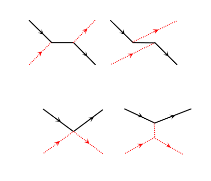
where the dots indicate 37 possible additional terms, involving schematically, either terms of the type , or of the type . Such a term would have to be added on the r.h.s. of the field equations in Eq. (10), and would therefore act as an additional source for the gravitational field (see Fig. 1). But the resulting field equations would then no longer invariant under Eq. (11), and one would have to change therefore the gauge transformation law by suitable terms of order , so as to ensure that the new field equations would still satisfy a local gauge invariance. In other words, all these complications arise because the gravitational field carries energy and momentum, and therefore gravitates.
Ultimately, a complete and satisfactory answer to these recursive attempts at constructing a consistent, locally gauge invariant, theory of the field is found in Einstein’s non-linear General Relativity theory, as shown in (Feynman, 1962; Boulware and Deser, 1969). The full theory is derived from the Einstein-Hilbert action
| (21) |
which generalized Eq. (7) beyond the weak field limit. Here is the square root of the determinant of the metric field , with , and the scalar curvature. The latter is related to the Ricci tensor and the Riemann tensor by
| (22) |
where is the matrix inverse of ,
| (23) |
In terms of the affine connection , the Riemann tensor is given by
| (24) |
and therefore
| (25) |
with the affine connection in turn constructed from components of the metric field
| (26) |
The following algebraic symmetry properties of the Riemann tensor will be of use later
| (27) |
| (28) |
| (29) |
In addition, the components of the Riemann tensor satisfy the differential Bianchi identities
| (30) |
with the covariant derivative. It is known that these, in their contracted form, ensure the consistency of the field equations. From the expansion of the Einstein-Hilbert gravitational action in powers of the deviation of the metric from the flat metric , using
| (31) |
one has for the action contribution
| (32) | |||||
again up to total derivatives. This last expression is in fact the same as Eq. (7). The correct relationship between the original graviton field and the metric field is
| (33) |
If, as is often customary, one rescales in such a way that the factor does not appear on the r.h.s., then both the and fields are dimensionless.
The weak field invariance properties of the gravitational action of Eq. (11) are replaced in the general theory by general coordinate transformations , under which the metric transforms as a covariant second rank tensor
| (34) |
which leaves the infinitesimal proper time interval with
| (35) |
invariant. In their infinitesimal form, coordinate transformations are written as
| (36) |
under which the metric at the same point then transforms as
| (37) |
and which is usually referred to as the Lie derivative of . The latter generalizes the weak field gauge invariance property of Eq. (11) to all orders in .
For infinitesimal coordinate transformations, one can gain some additional physical insight by decomposing the derivative of the small coordinate change in Eq. (36) as
| (38) |
with
| (39) |
Then can be thought of describing local scale transformations, is written in terms of an antisymmeric tensor and therefore describes local rotations, while contains a traceless symmetric tensor and describes local shears.
Since both the scalar curvature and the volume element are separately invariant under the general coordinate transformations of Eqs. (34) and (36), both of the following action contributions are acceptable
| (40) |
the first being known as the cosmological constant contribution (as it represents the total space-time volume). In the weak field limit, the first, cosmological constant term involves
| (41) |
which is easily obtained from the matrix formula
| (42) |
after expanding out the exponential in powers of . We have also reverted here to the more traditional way of performing the weak field expansion (i.e. without factors of ),
| (43) |
with the flat metric. The reason why such a cosmological consant term was not originally included in the construction of the Lagrangian of Eq. (7) is that it does not contain derivatives of the field. It is in a sense analogous to a mass term, without giving rise to any breaking of local gauge invariance.
In the general theory, the energy-momentum tensor for matter is most suitably defined in terms of the variation of the matter action ,
| (44) |
and is conserved if the matter action is a scalar,
| (45) |
Variation of the gravitational Einstein-Hilbert action of Eq. (21), with the matter part added, then leads to the field equations
| (46) |
Here we have also added a cosmological constant term, with a scaled cosmological constant , which follows from adding to the gravitational action a term 111 The present experimental value for Newton’s constant is . Recent observational evidence [reviewed in (Damour,2007)] suggests a non-vanishing positive cosmological constant , corresponding to a vacuum density with related to by . As can be seen from the field equations, has the same dimensions as a curvature. One has from observation , so this new curvature length scale is comparable to the size of the visible universe . .
One can exploit the freedom under general coordinate transformations to impose a suitable coordinate condition, such as
| (47) |
which is seen to be equivalent to the following gauge condition on the metric
| (48) |
and therefore equivalent, in the weak field limit, to the harmonic gauge condition introduced previously in Eq. (12).
II.1.3 Feynman Rules
The Feynman rules represent the standard way to do perturbative calculations in quantum gravity. To this end one first expands again the action out in powers of the field and separates out the quadratic part, which gives the graviton propagator, from the rest of the Lagrangian which gives the vertices. To define the graviton propagator one also requires the addition of a gauge fixing term and the associated Faddeev-Popov ghost contribution (Feynman, 1962; Faddeev and Popov, 1968). Since the diagrammatic calculations are performed using dimensional regularization, one first needs to define the theory in dimensions; at the end of the calculations one will be interested in the limit .
So first one expands around the -dimensional flat Minkowski space-time metric, with signature given by . The Einstein-Hilbert action in dimensions is given by a generalization of Eq. (21)
| (49) |
with again and the scalar curvature; in the following it will be assumed, at least initially, that the bare cosmological constant is zero. The simplest form of matter coupled in an invariant way to gravity is a set of spinless scalar particles of mass , with action
| (50) |
In Feynman diagram perturbation theory the metric is expanded around the flat metric , by writing again
| (51) |
The quadratic part of the Lagrangian [see Eq. (7)] is then
| (52) |
where the dots indicate terms that are either total derivatives, or higher order in . A suitable gauge fixing term is given by
| (53) |
Without such a term the quadratic part of the gravitational Lagrangian of Eq. (7) would contain a zero mode , due to the gauge invariance of Eq. (11), which would make the graviton propagator ill defined.
The gauge fixing contribution itself will be written as the sum of two terms,
| (54) |
with the first term engineered so as to conveniently cancel the in Eq. (52) and thus give a well defined graviton propagator. Note incidentally that this gauge is not the harmonic gauge condition of Eq. (12), and is usually referred to instead as the DeDonder gauge. The second term is determined as usual from the variation of the gauge condition under an infinitesimal gauge transformation of the type in Eq. (11)
| (55) |
which leads to the lowest order ghost Lagrangian
| (56) |
where is the spin-one anticommuting ghost field, with propagator
| (57) |
In this gauge the graviton propagator is finally determined from the surviving quadratic part of the pure gravity Lagrangian, which is
| (58) |
The latter can be conveniently re-written in terms of a matrix
| (59) |
with
| (60) |
The matrix can easily be inverted, for example by re-labelling rows and columns via the correspondence
| (61) |
and the graviton Feynman propagator in dimensions is then found to be of the form
| (62) |
with a suitable prescription to correctly integrate around poles in the complex space. Equivalently the whole procedure could have been performed from the start with an Euclidean metric and a complex time coordinate with hardly any changes of substance. The simple pole in the graviton propagator at serves as a reminder of the fact that, due to the Gauss-Bonnet identity, the gravitational Einstein-Hilbert action of Eq. (49) becomes a topological invariant in two dimensions.
Higher order correction in to the Lagrangian for pure gravity then determine to order the three-graviton vertex, to order the four-graviton vertex, and so on. Because of the and terms in the action, there are an infinite number of vertices in .
Had one included a cosmological constant term as in Eq. (41), which can also be expressed in terms of the matrix as
| (63) |
then the the expression in Eq. (59) would have read
| (64) |
with . Then the graviton propagator would have been remained the same, except for the replacement . In this gauge it would correspond to the exchange of a particle of mass . The term linear in can be interpreted as a uniform constant source for the gravitational field. But one needs to be quite careful, since for non-vanishing cosmological constant flat space is no longer a solution of the vacuum field equations and the problem becomes a bit more subtle: one needs to expand around the correct vacuum solutions in the presence of a -term, which are no longer constant.
Another point needs to be made here. One peculiar aspect of perturbative gravity is that there is no unique way of doing the weak field expansions, and one can have therefore different sets of Feynman rules, even apart from the choice of gauge condition, depending on how one chooses to do the expansion for the metric.
For example, the structure of the scalar field action of Eq. (50) suggests to define instead the small fluctuation graviton field via
| (65) |
with (Faddeev and Popov, 1973; Capper et al, 1973). Here it is that should be referred to as ”the graviton field”. The change of variables from the ’s to the ’s involves a Jacobian, which can be taken to be one in dimensional regularization. There is one obvious advantage of this expansion over the previous one, namely that it leads to considerably simpler Feynman rules, both for the graviton vertices and for the scalar-graviton vertices, which can be advantageous when computing one-loop scattering amplitudes of scalar particles (Hamber and Liu, 1985). Even the original gravitational action has a simpler form in terms of the variables of Eq. (65) as shown originally in (Goldberg, 1958).
Again, when performing Feynman diagram perturbation theory a gauge fixing term needs to be added in order to define the propagator, for example of the form
| (66) |
In this new framework the bare graviton propagator is given simply by
| (67) |
which should be compared to Eq. (62) (the extra factor of one half here is just due to the convention in the choice of ). One notices that now there are no factors of for the graviton propagator in dimensions. But such factors appear instead in the expression for the Feynman rules for the graviton vertices, and such pole terms appear therefore regardless of the choice of expansion field. For the three-graviton and two ghost-graviton vertex the relevant expressions are quite complicated. The three-graviton vertex is given by
The ghost-graviton vertex is given by
| (69) |
and the two scalar-one graviton vertex is given by
| (70) |
where the denote the four-momenta of the incoming and outgoing scalar field, respectively. Finally the two scalar-two graviton vertex is given by
| (71) |
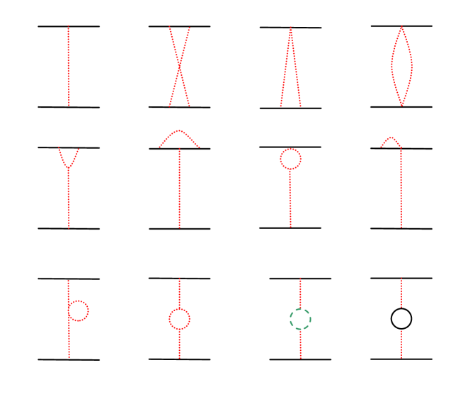
where one pair of indices is associated with one graviton line, and the other pair is associated with the other graviton line. These rules follow readily from the expansion of the gravitational action to order (), and of the scalar field action to order (), as shown in detail in (Capper et al, 1973). Note that the poles in have disappeared from the propagator, but have moved to the vertex functions. As mentioned before, they reflect the kinematic singularities that arise in the theory as due to the Gauss-Bonnet identity. As an illustration, Fig. 2 shows the lowest order diagrams contributing to the static potential between two massive spinless sources (Hamber and Liu, 1995).
II.1.4 One-Loop Divergences
Once the propagators and vertices have been defined, one can then proceed as in QED and Yang-Mills theories and evaluate the quantum mechanical one loop corrections. In a renormalizable theory with a dimensionless coupling, such as QED and Yang-Mills theories, one has that the radiative corrections lead to charge, mass and field re-definitions. In particular, for the pure gauge action one finds
| (72) |
so that the form of the action is preserved by the renormalization procedure: no new interaction terms such as need to be introduced in order to re-absorb the divergences.
In gravity the coupling is dimensionful, , and one expects trouble already on purely dimensional grounds, with divergent one loop corrections proportional to where is an ultraviolet cutoff 222 Indeed it was noticed very early on in the development of renormalization theory that perturbatively non-renormalizible theories would involve couplings with negative mass dimensions, and for which cross sections would grow rapidly with energy (Sakata, Umezawa and Kamefuchi, 1952). It had originally been suggested by Heisenberg (Heisenberg, 1938) that the relevant mass scale appearing in such interactions with dimensionful coupling constants should be used to set an upper energy limit on the physical applicability of such theories. . Equivalently, one expects to lowest order bad ultraviolet behavior for the running Newton’s constant at large momenta,
| (73) |
These considerations also suggest that perhaps ordinary Einstein gravity is perturbatively renormalizable in the traditional sense in two dimensions, an issue to which we will return later in Sect. II.3.4.
A more general argument goes as follows. The gravitational action contains the scalar curvature which involves two derivatives of the metric. Thus the graviton propagator in momentum space will go like , and the vertex functions like . In dimensions each loop integral with involve a momentum integration , so that the superficial degree of divergence of a Feynman diagram with vertices, internal lines and loops will be given by
| (74) |
The topological relation involving , and
| (75) |
is true for any diagram, and yields
| (76) |
which is independent of the number of external lines. One concludes therefore that for the degree of divergence increases with increasing loop order .
The most convenient tool to determine the structure of the divergent one-loop corrections to Einstein gravity is the background field method (DeWitt, 1967; ’t Hooft and Veltman, 1974) combined with dimensional regularization, wherein ultraviolet divergences appear as poles in 333The second reference uses a complex time (Euclidean) notation that differs from the one used here.. In non-Abelian gauge theories the background field method greatly simplifies the calculation of renormalization factors, while at the same time maintaining explicit gauge invariance.
The essence of the method is easy to describe: one replaces the original field appearing in the classical action by , where is a classical background field and the quantum fluctuation. A suitable gauge condition is chosen (the background gauge), such that manifest gauge invariance is preserved for the background field. After expanding out the action to quadratic order in the field, the functional integration over is performed, leading to an effective action for the background field. From the structure of this effective action the renormalization of the couplings, as well as possible additional counterterms, can then be read off. In the case of gravity it is in fact sufficient to look at the structure of those terms appearing in the effective action which are quadratic in the background field . A very readable introduction to the background field method as applied to gauge theories can be found in (Abbot, 1981).
Unfortunately perturbative calculations in gravity are rather cumbersome due to the large number of indices and contractions, so the rest of this section is only intended more as a general outline, with the scope of hopefully providing some of the flavor of the original calculations. The first step consists in the replacement
| (77) |
where now is the classical background field and the quantum field, to be integrated over. To determine the structure of one loop divergences it will often be sufficient to consider at the very end just the case of a flat background metric, , or a small deviation from it.
After a somewhat tedious calculation one finds for the bare action
| (78) |
expanded out to quadratic order in
up to total derivatives. Here denotes a covariant derivative with respect to the metric . For the above expression coincides with the weak field Lagrangian contained in Eqs. (7) and (52), with a cosmological constant term added, as given in Eq. (41).
To this expression one needs to add the gauge fixing and ghost contributions, as was done in Eq. (52). The background gauge fixing term used is
| (80) |
with a corresponding ghost Lagrangian
| (81) |
The integration over the field can then be performed with the aid of the standard Gaussian integral formula
| (82) |
leading to an effective action for the field. In practice one is only interested in the divergent part, which can be shown to be local. Specific details of the functional measure over metrics are not deemed to be essential at this stage, as in perturbation theory one is only doing Gaussian integrals, with ranging from to . In particular when using dimensional regularization one uses the formal rule
| (83) |
which leads to some technical simplifications but obscures the role of the measure.
In the flat background field case case , the functional integration over the fields would have been particularly simple, since then one would be using
| (84) |
with the graviton propagator given in Eq. (62). In practice, one can use the expected generally covariant structure of the one-loop divergent part
| (85) |
with and some real parameters, as well as its weak field form, obtained from
[compare with Eq. (31)], combined with some suitable special choices for the background metric, such as , to further simplify the calculation. This eventually determines the required one-loop counterterm for pure gravity to be
| (87) |
For the simpler case of classical gravity coupled invariantly to a single real quantum scalar field one finds
| (88) |
The complete set of one-loop divergences, computed using the alternate method of the heat kernel expansion and zeta function regularization 444 The zeta-function regularization (Hawking, 1977) involves studying the behavior of the function , where the ’s are the eigenvalues of the second order differential operator in question. The series will converge for , and can be used for an analytic continuation to , which then leads to the formal result . close to four dimensions, can be found in the comprehensive review (Hawking, 1977) and further references therein. In any case one is led to conclude that pure quantum gravity in four dimensions is not perturbatively renormalizable: the one-loop divergent part contains local operators which were not present in the original Lagrangian. It would seem therefore that these operators would have to be added to the bare , so that a consistent perturbative renormalization program can be developed in four dimensions.
There are two interesting, and interrelated, aspects of the result of Eq. (87). The first one is that for pure gravity the divergent part vanishes when one imposes the tree-level equations of motion : the one-loop divergence vanishes on-shell. The second interesting aspect is that the specific structure of the one-loop divergence is such that its effect can actually be re-absorbed into a field redefinition,
| (89) | |||||
which renders the one-loop amplitudes finite for pure gravity. Unfortunately this hoped-for mechanism does not seem to work to two loops, and no additional miraculous cancellations seem to occur there. At two loops one expects on general grounds terms of the type , and . It can be shown that the first class of terms reduce to total derivatives, and that the second class of terms can also be made to vanish on shell by using the Bianchi identity. Out of the last set of terms, the ones, one can show (’t Hooft, 2002) that there are potentially 20 distinct contributions, of which 19 vanish on shell (i.e. by using the tree level field equations ). An explicit calculation then shows that a new non-removable on-shell -type divergence arises in pure gravity at two loops (Goroff and Sagnotti, 1985; van de Ven, 1992) from the only possible surviving non-vanishing counterterm, namely
| (90) |
To summarize, radiative corrections to pure Einstein gravity without a cosmological constant term induce one-loop -type divergences of the form
| (91) |
and a two-loop non-removable on-shell -type divergence of the type
| (92) |
which present an almost insurmountable obstacle to the traditional perturbative renormalization procedure in four dimensions. One can therefore attempt to summarize the situation so far as follows:
-
In principle perturbation theory in in provides a clear, covariant framework in which radiative corrections to gravity can be computed in a systematic loop expansion. The effects of a possibly non-trivial gravitational measure do not show up at any order in the weak field expansion, and radiative corrections affecting the renormalization of the cosmological constant, proportional to , are set to zero in dimensional regularization.
-
At the same time at every order in the loop expansion new invariant terms involving higher derivatives of the metric are generated, whose effects cannot be simply re-absorbed into a re-definition of the original couplings. As expected on the basis of power-counting arguments, the theory is not perturbatively renormalizable in the traditional sense in four dimensions (although it seems to fail this test by a small measure in lowest order perturbation theory).
-
The standard approach based on a perturbative expansion of the pure Einstein theory in four dimensions is therefore not convergent (it is in fact badly divergent), and represents therefore a temporary dead end.
II.1.5 Higher Derivative Terms
In the previous section it was shown that quantum corrections to the Einstein theory generate in perturbation theory -type terms in four dimensions. It seems therefore that, for the consistency of the perturbative renormalization group approach in four dimension, these terms would have to be included from the start, at the level of the bare microscopic action. Thus the main motivation for studying gravity with higher derivative terms is that it might cure the problem of ordinary quantum gravity, namely its perturbative non-renormalizabilty in four dimensions. This is indeed the case, in fact one can prove that higher derivative gravity (to be defined below) is perturbatively renormalizable to all orders in four dimensions.
At the same time new issues arise, which will be detailed below. The first set of problems has to do with the fact that, quite generally higher derivative theories with terms of the type suffer from potential unitarity problems, which can lead to physically unacceptable negative probabilities. But since these are genuinely dynamical issues, it will be difficult to answer them satisfactorily in perturbation theory. In non-Abelian gauge theories one can use higher derivative terms, instead of the more traditional dimensional continuation, to regulate ultraviolet divergences (Slavnov, 1973), and higher derivative terms have been used successfully for some time in lattice regulated field theories (Symanzik, 1983). In these approaches the coefficient of the higher derivative terms is taken to zero at the end. The second set of issues is connected with the fact that the theory is asymptotically free in the higher derivative couplings, implying an infared growth which renders the perturbative estimates unreliable at low energies, in the regime of perhaps greatest physical interest. Note that higher derivative terms arise in string theory as well (Förger, Ovrut, Theisen and Waldram, 1996).
Let us first discuss the general formulation. In four dimensions possible terms quadratic in the curvature are
| (93) |
where is the Euler characteristic and the Hirzebruch signature. It will be shown below that these quantities are not all independent. The Weyl conformal tensor is defined in dimensions as
| (94) | |||||
where square brackets denote antisymmetrization. It is called conformal because it can be shown to be invariant under conformal transformations of the metric, . In four dimensions one has
| (95) |
The Weyl tensor can be regarded as the traceless part of the Riemann curvature tensor,
| (96) |
and on-shell the Riemann tensor in fact coincides with the Weyl tensor. From the definition of the Weyl tensor one infers in four dimensions the following curvature-squared identity
| (97) |
Some of these results are specific to four dimensions. For example, in three dimensions the Weyl tensor vanishes identically and one has
| (98) |
In four dimensions the expression for the Euler characteristic can be written equivalently as
| (99) |
The last result is the four-dimensional analog of the two-dimensional Gauss-Bonnet formula
| (100) |
where and is the genus of the surface (the number of handles). For a manifold of fixed topology one can therefore use in four dimensions
| (101) |
and
| (102) |
Thus only two curvature squared terms for the gravitational action are independent in four dimensions (Lanczos, 1938), which can be chosen, for example, to be and . Consequently the most general curvature squared action in four dimensions can be written as
| (103) |
with , and up to boundary terms. The case corresponds, by virtue of Eq. (102), to the conformally invariant, pure Weyl-squared case. If then around flat space one encounters a tachyon at tree level. It will also be of some interest later that in the Euclidean case (signature ) the full gravitational action of Eq. (103) is positive for , and .
Curvature squared actions for classical gravity were originally considered in (Weyl, 1922) and (Pauli, 1956). In the sixties it was argued that the higher derivative action of Eq. (103) should be power counting renormalizable (Utiyama and DeWitt, 1961). Later it was proven to be renormalizable to all orders in perturbation theory (Stelle, 1977). Some special cases of higher derivative theories have been shown to be classically equivalent to scalar-tensor theories (Whitt 1984).
One way to investigate physical properties of higher derivative theories is again via the weak field expansion. In analyzing the particle content it is useful to introduce a set of spin projection operators (Arnowitt, Deser and Misner, 1958; van Nievenhuizen, 1973), quite analogous to what is used in describing transverse-traceless (TT) modes in classical gravity (Misner, Thorne and Wheeler, 1973). These projection operators then show explicitly the unique decomposition of the continuum gravitational action for linearized gravity into spin two (transverse-traceless) and spin zero (conformal mode) parts. The spin-two projection operator is defined in -space as
| (104) | |||||
the spin-one projection operator as
| (105) | |||||
and the spin-zero projection operator as
| (106) | |||||
It is easy to check that the sum of the three spin projection operators adds up to unity
| (107) |
These projection operators then allow a decomposition of the gravitational field into three independent modes. The spin two or transverse-traceless part
| (108) |
the spin one or longitudinal part
| (109) |
and the spin zero or trace part
| (110) |
are such that their sum gives the original field
| (111) |
with the quantity defined as
| (112) |
or, equivalently, in -space .
One can learn a number of useful aspects of the theory by looking at the linearized form of the equations of motion. As before, the linearized form of the action is obtained by setting and expanding in . Besides the expressions given in Eq. (31), one needs
| (113) |
from which one can then obtain, for example from Eq. (101), an expression for ,
Using the three spin projection operators defined previously, the action for linearized gravity without a cosmological constant term, Eq. (7), can then be re-expressed as
| (115) |
Only the and projection operators for the spin-two and spin-zero modes, respectively, appear in the action for the linearized gravitational field; the spin-one gauge mode does not enter the linearized action. Note also that the spin-zero mode enters with the wrong sign (in the linearized action it appears as a ghost contribution), but to this order it can be removed by a suitable choice of gauge in which the trace mode is made to vanish, as can be seen, for example, from Eq. (13).
It is often stated that higher derivative theories suffer from unitarity problems. This is seen as follows. When the higher derivative terms are included, the corresponding linearized expression for the gravitational action becomes
| (116) | |||||
Then the potential problems with unitarity and ghosts at ultrahigh energies, say comparable to the Planck mass , can be seen by examining the graviton propagator (Salam and Strathdee, 1978). In momentum space the free graviton propagator for higher derivative gravity and can be written as
| (117) |
The first two terms on the r.h.s. can be decomposed as
| (118) |
One can see that, on the one hand, the higher derivative terms improve the ultraviolet behavior of the theory, since the propagator now falls of as for large . At the same time, the theory appears to contain a spin-two ghost of mass and a spin-zero particle of mass . Here we have set , which is of the order of the Planck mass (). For one finds a tachyon pole, which seems, for the time being, to justify the original choice of in Eq. (103).
Higher derivative gravity theories also lead to modifications to the standard Newtonian potential, even though such deviations only become visible at very short distances, comparable to the Planck length . In some special cases they can be shown to be classically equivalent to scalar-tensor theories without higher derivative terms (Whitt, 1984). The presence of massive states in the tree level graviton propagator indicates short distance deviations from the static Newtonian potential of the form
| (119) |
Moreover in the extreme case corresponding to the absence of the Einstein term () the potential is linear in ; but in this limit the theory is strongly infrared divergent, and it is not at all clear whether weak coupling perturbation theory is of any relevance.
In the quantum theory perturbation theory is usually performed around flat space, which requires , or around some fixed classical background. One sets again and expands the higher derivative action in powers of . If is nonzero, one has to expand around a solution of the classical equations of motion for higher derivative gravity with a -term (Barth and Christensen, 1983), and the solution will no longer be constant over space-time. The above expansion is consistent with the assumption that the two higher derivative couplings and are large, since in such a limit one is close to flat space. One-loop radiative corrections then show that the theory is asymptotically free in the higher derivative couplings and (Julve and Tonin, 1978; Fradkin and Tseytlin, 1981; Avramidy and Barvinsky, 1985).
The calculation of one-loop quantum fluctuation effects proceeds in a way that is similar to the pure Einstein gravity case. One first decomposes the metric field as a classical background part and a quantum fluctuation part as in Eq. (77), and then expands the classical action to quadratic order in , with gauge fixing and ghost contributions added, similar to those in Eqs. (80) and (81), respectively. The first order variation of the action of Eq. (103) gives the field equations for higher derivative gravity in the absence of sources,
| (120) | |||||
where we have set for the ratio of the two higher derivative couplings .
The second order variation is done similarly. It then allows the Gaussian integral over the quantum fields to be performed using the formula of Eq. (82). One then finds that the one-loop effective action, which depends on only, can be expressed as
| (121) |
with the quantities and defined by
| (122) |
A shorthand notation is used here, where spacetime and internal indices are grouped together so that . are a set of gauge conditions, is a nonsingular functional matrix fixing the gauge, and the are the local generators of the group of general coordinate transformations, .
Ultimately one is only interested in the divergent part of the effective one-loop action. The method of extracting the divergent part out of the determinant (or trace ) expression in Eq. (121) is similar to what is done, for example, in QED to evaluate the contribution of the fermion vacuum polarization loop to the effective action. There, after integrating out the fermions, one obtains a functional determinant of the massless Dirac operator in an external field,
| (123) |
with a calculable numerical constant. The trace needs to be regulated, and one way of doing it is via the integral representation
| (124) |
with a cutoff that is sent to zero at the end of the calculation. For gauge theories a detailed discussion can be found for example in (Rothe, 1985), and references therein. In the gravity case further discussions and more results can be found in (De Witt 1965; ’t Hooft and Veltman 1974; Gilkey 1975; Christensen and Duff 1979) and references therein.
In the end, by a calculation similar to the one done in the pure Einstein gravity case, one finds that the one-loop contribution to the effective action contains for a divergent term of the form
| (125) |
with the coefficients for the divergent parts given by
| (126) |
Here and is the dimensionless combination of the cosmological and Newton’s constant with . A divergence proportional to the topological invariant with coefficient has not been included, as it only adds a field-independent constant to the action for a manifold of fixed topology. Also -type divergences possibly originating from a non-trivial functional measure over the ’s have been set to zero.
The structure of the ultraviolet divergences (which for an explicit momentum cutoff would have appeared as ) allow one to read off immediately the renormalization group -functions for the various couplings. To this order, the renormalization group equations for the two higher derivative couplings and and the dimensionless ratio of cosmological and Newton’s constant are
| (127) |
with the dots indicating higher loop corrections. Here is the logarithm of the relevant energy scale, , with a momentum scale , and some fixed reference scale. It is argued furthermore by the quoted authors that only the quantities , and the combination are gauge independent, the latter combination appearing in the renormalization group equation for (this is a point to which we shall return later, as it follows quite generally from the properties of the gravitational action, and therefore from the gravitational functional integral, under a field rescaling, see Sect. II.3.4).
The perturbative scale dependence of the couplings , and follows from integrating the three differential equations in Eq. (127). The first renormalization group equation is easily integrated, and shows the existence of an ultraviolet fixed point at ; the one-loop result for the running coupling is simply given by , or
| (128) |
with a reference scale. It suggests that the effective higher derivative coupling increases at short distances, but decreases in the infrared regime . But one should keep in mind that the one loop results are reliable at best only at very short distances, or large energy scales, . At the same time these results seem physically reasonable, as one would expect curvature squared terms to play less of a role at larger distances, as in the classical theory.
The scale dependence of the other couplings is a bit more complicated. The equation for exhibits two fixed points at and ; in either case this would correspond to a higher derivative action with a positive term. It would also give rise to rapid short distance oscillations in the static potential, as can be seen for example from Eq. (119) and the definition of . The equation for gives a solution to one-loop order with , suggesting that the effective gravitational constant, in units of the cosmologial constant, decreases at large distances. The experimental value for Newton’s constant and for the scaled cosmological constant is such that the observed dimensionless ratio between the two is very small, . In the present model is seems entirely unclear how such a small ratio could arise from perturbation theory alone.
At short distances the dimensionless coupling seems to increases rapidly, thus partially invalidating the conclusions of a weak field expansion around flat space, which are based generally on the assumption of small and . At the same time, the fact that the higher derivative coupling grows more rapidly in the ultraviolet than the coupling can be used retroactively at least as a partial justification for the flat space expansion, in which the cosmological and Einstein terms are treated perturbatively. Ultimately the resolution of such delicate and complex issues would presumably require the development of the perturbative expansion not around flat space, but more appropriately around the de Sitter metric, for which . Even then one would have to confront such genuinely non-perturbative issues, such as what happens to the spin-zero ghost mass, whether the ghost poles gets shifted away from the real axis by quantum effects, and what the true ground state of the theory looks like in the long distance, strong fluctuation regime not accessible by perturbation theory.
What is also a bit surprising is that higher derivative gravity, to one-loop order, does not exhibit a nontrivial ultraviolet point in , even though such a fixed point is clearly present in the expansion (to be discussed later) at the one- and two-loop order, as well as in the lattice regularized theory in four dimensions (also to be discussed later). But this could just reflect a limitation of the one-loop calculation; to properly estimate the uncertainties of the perturbative results in higher derivative gravity and their potential physical implications a two-loop calculation is needed, which hopefully will be performed in the near future.
To summarize, higher derivative gravity theories based on -type terms are perturbatively renormalizable, but exhibit some short-distance oddities in the tree-level spectrum, associated with either ghosts or tachyons. Their perturbative (weak field) treatment suggest that the higher derivative couplings are only relevant at short distances, comparable to the Planck length, but the general evolution of the couplings away from a regime where perturbation theory is reliable remains an open question, which perhaps will never be answered satisfactorily in perturbation theory, if non-Abelian gauge theories, which are also asymptotically free, are taken as a guide.
II.1.6 Supergravity
An alternative approach to the vexing problem of ultraviolet divergences in perturbative quantum gravity (and for that matter, in any field theory) is to build in some additional degree of symmetry, such that loop effects acquire reduced divergence properties, or even become finite. One such approach, based on the invariance under local supersymmetry transformation, adds to the Einstein gravity Lagrangian a spin- gravitino field, whose purpose is to exactly cancel the loop divergences in the Einstein contributions. The enhanced symmetry is built in to ensure that such a cancellation does not just occur at one loop order, but propagates to every order of the loop expansion. The intent of this section is more to provide the general flavor of such an approach, and illustrate supergravity theories by a few specific examples of suitable actions. The reader is then referred to the vast literature on the subject for further examples, as well as contemporary leading candidate theories.
In the simplest scenario, one adds to gravity a spin- fermion field with suitable symmetry properties. A generally covariant action describing the interaction of vierbein fields (with the metric field given by ) and Rarita-Schwinger spin- fields , subject to the Majorana constraints , was originally given in (Ferrara, Freedman and van Nieuwenhuizen, 1976). In the second order formulation it contains three contributions
| (129) |
with the usual Einstein term
| (130) |
the gravitino contribution
| (131) |
and a quartic fermion self-interaction
| (132) | |||||
The covariant derivative defined as
| (133) |
involves the standard affine connection , as well as the vierbein connection
| (134) | |||||
with Dirac spin matrices
| (135) |
One can show that the combined Lagrangian is invariant, up to terms of order , under the simultaneous transformations
| (136) |
where in an arbitrary Majorana spinor.
The action of Eq. (129) can be written equivalently in first order form (Deser and Zumino, 1976) as
| (137) |
with the vierbein with , and
| (138) |
The covariant derivative on is defined in terms of its spin- part only
| (139) |
and is related to the curvature tensor via the commutator identity
| (140) |
The first order action in Eq. (137) is invariant under
| (141) |
with the quantity defined as
| (142) |
and in an arbitary local Majorana spinor. In the first order formulation the vierbeins , the connections and the Majorana vector-spinors are supposed to be varied independently.
In (D’Eath, 1984; 1994) the supergravity action is written as
| (143) |
with
| (144) |
| (145) |
in terms of the Weyl spinor gravitino fields and and the vierbein field . The ’s are Levi-Civita symbols with curved (up) and flat (down) indices respectively. The quantities represent a curved space generalization of the Pauli matrices discussed in (Carroll et al, 1994).
The original motivation for the supergravity action of Eqs. (129) or (137) was that, just like ordinary source-free gravity is ultraviolet finite on-shell because of the identity relating the invariant to and , identities among invariants constructed out of and the strong constraints of supersymmetry would ensure one-loop, and higher, renormalizabilty of supergravity. There are reasons to believe that the triviality results found originally in globally supersymmetric theories (Nicolai, 1984) will not carry over into theories with local supersymetry.
It was shown originally in (Grisaru, van Nieuwenhuizen and Vermaseren, 1976) and (Grisaru, 1976) that the original supergravity theory is finite to at least two loops. But most likely it fails to be finite at three loops (Deser, Kay and Stelle, 1977). As a consequence, more complex theories were devised to avoid the three-loop catastrophe. A new formulation, extended supergravity based on an symmetry, was suggested in (Das 1977; Cremmer and Scherk, 1977; Nicolai and Townsend, 1981). This theory now contains vector, spinor and scalar particle in addition to the gravitino and the graviton. Specifically, the theory contains a vierbein field , four spin- Majorana fields , four spin- Majorana fields , six vector fields , a scalar field and a pseudoscalar field , all massless, for a grand total of 53 independent terms in the Lagrangian. Subsequently supergravity was proposed, based on the even larger group (Cremmer and Julia, 1978). The enlarged theory now contains one graviton, 8 gravitinos, 28 vector fields, 56 Majorana spin- fields and 70 scalar fields, all massless. In general, supergravity contains gravitinos, gauge fields, as well as several spin- Majorana fermions and complex scalars. The symmetry here is one which rotates, for example, the gravitinos into each other. In (Christensen, Duff, Gibbons and Roc̆ek, 1980) it was shown that in general such theories are finite at one loop order for . For these theories become less viable since one then has more than one graviton, which leads to paradoxes, as well as particles with spin .
It is beyond our scope here to go any more deeply in the issue of the origin of such intriguing ultraviolet cancellations. But, as perhaps the simplest and most elementary motivation, one can use the Nielsen-Hughes formula (Nielsen, 1980; Hughes, 1981) for the one-loop -function contribution from a particle of spin
| (146) |
to verify, by virtue of the particle multiplicities given above, that for example for the lowest order divergences cancel
| (147) |
For one has a similar complete cancellation
| (148) |
Still, the issue of perturbative ultraviolet finiteness of these theories remains largely an open question, in part due to the daunting complexity of higher loop calculations, even though one believes that the high level of symmetry should ensure the cancellation of ultraviolet divergences to a very high order (at least up to seven loops). Recently it was suggested, based on the correspondence between supergravity and super Yang-Mills theory and the cancellations which arise at one and higher loops, that supergravity theories might be finite to all orders in the loop expansion (Bern, Dixon and Roiban, 2006).
One undoubtedly very attractive feature of supergravity theories is that they lead naturally to a small, or even vanishing, renormalized cosmological constant . Due to the high level of symmetry, quartic and quadratic divergences in this quantity are expected to cancel exactly between bosonic and fermionic contributions, leaving a finite or even zero result. The hope is that some of these desirable features will survive supersymmetry breaking, a mechanism eventually required in order to remove, or shift to a high mass, the so far unobserved supersymmetric partners of the standard model particles.
II.2 Feynman Path Integral Formulation
So far the discussion of quantum gravity has focused almost entirely on perturbative aspects, where the gravitational coupling is assumed to be weak, and the weak field expansion based on can be performed with some degree of reliability. At every order in the loop expansion the problem then reduces to the systematic evaluation of an increasingly complex sequence of Gaussian integrals over the (small) quantum fluctuation .
But there are reasons to expect that non-perturbative effects play an important role in quantum gravity. Then an improved formulation of the quantum theory is required, which does not rely exclusively on the framework of a perturbative expansion. Indeed already classically a black hole solution can hardly be considered a small perturbation of flat space. Furthermore, the fluctuating metric field is dimensionless and carries therefore no natural scale. For the simpler cases of a scalar field and non-Abelian gauge theories a consistent non-perturbative formulation based on the Feynman path integral has been known for some time and is well developed. Combined with the lattice approach, it provides an effective and powerful tool for systematically investigating non-trivial strong coupling behavior, such as confinement and chiral symmetry breaking. These phenomena are known to be generally inaccessible in weak coupling perturbation theory. In addition, the Feynman path integral approach provides a manifestly covariant formulation of the quantum theory, without the need for an artificial split required by the more traditional canonical approach, and the ambiguities that may follow from it. In fact, as will be seen later, in its non-perturbative lattice formulation no gauge fixing is required.
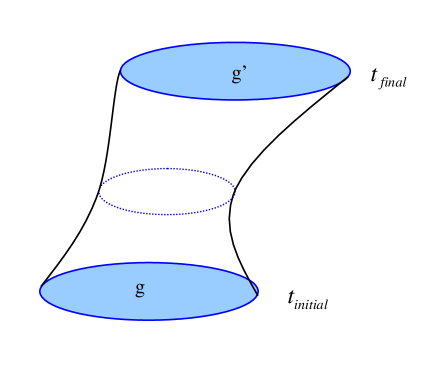
In a nutshell, the Feynman path integral formulation for pure quantum gravitation can be expressed in the functional integral formula
| (149) |
(for an illustration see Fig. 3), just like the Feynman path integral for a non-relativistic quantum mechanical particle (Feynman, 1951; Feynman and Hibbs, 1962) expresses quantum-mechanical amplitudes in terms of sums over paths
| (150) |
What is the precise meaning of the expression in Eq. (149)? The remainder of this section will be devoted to discussing attempts at a proper definition of the gravitational path integral of Eq. (149). A modern rigorous discussion of path integrals in quantum mechanics and (Euclidean) quantum field theory can be found, for example, in (Albeverio and Hoegh-Krohn, 1976), (Glimm and Jaffe, 1981), and (Zinn-Justin, 2002).
II.2.1 Sum over Paths
Already for a non-relativistic particle the path integral needs to be defined quite carefully by discretizing the time and introducing a short distance cutoff. The standard procedure starts from the quantum-mechanical transition amplitude
| (151) |
and subdivides the time interval into segments of size with . Using completeness of the coordinate basis at all intermediate times, one obtains the textbook result, here for a non-relativistic particle described by a Hamiltonian ,
| (152) | |||||
The expression in the exponent is recognized as a discretized form of the classical action. The above quantum-mechanical amplitude is usually written in shorthand as
| (153) |
with the Lagrangian for the particle. Thus what appears in the exponent is the classical action
| (154) |
associated with a given trajectory , connecting the initial coordinate with the final one . Then is the functional measure over paths , as spelled out explicitly in the precise lattice definition of Eq. (152). One advantage associated with having the classical action appear in the quantum mechanical amplitude is that all the symmetries of the theory are manifest in the Lagrangian form. The symmetries of the Lagrangian then have direct implications for the study of quantum mechanical amplitudes. A stationary phase approximation to the path integral, valid in the limit , leads to the least action principle of classical mechanics
| (155) |
In the above derivation it is not necessary to use a uniform lattice spacing ; one could have used as well a non-uniform spacing but the result would have been the same in the limit (in analogy with the definition of the Riemann sum for ordinary integrals). Since quantum mechanical paths have a zig-zag nature and are nowhere differentiable, the mathematically correct definition should be taken from the finite sum in Eq. (152). In fact it can be shown that differentiable paths have zero measure in the Feynman path integral: already for the non-relativistic particle most of the contributions to the path integral come from paths that are far from smooth on all scales (Feynman and Hibbs, 1963), the so-called Wiener paths in turn related to Brownian motion. In particular, the derivative is not always defined, and the correct definition for the path integral is the one given in Eq. (152). A very complete and contemporary reference to the many applications of path integrals to non-relativistic quantum systems and statistical physics can be found in two recent books (Zinn-Justin, 2003; Kleinert, 2006).
As a next step, one can generalized the Feynman path integral construction to particles with coordinates (), and finally to the limiting case of continuous fields . If the field theory is defined from the start on a lattice, then the quantum fields are defined on suitable lattice points as .
II.2.2 Eulidean Rotation
In the case of quantum fields, one is generally interested in the vacuum-to-vacuum amplitude, which requires and . Then the functional integral with sources is of the form
| (156) |
where , and the usual Lagrangian density for the scalar field,
| (157) |
However even with an underlying lattice discretization, the integral in Eq. (156) is in general ill-defined without a damping factor, due to the in the exponent (Zinn-Justin, 2003).
Advances in axiomatic field theory (Osterwalder and Schrader, 1973; Glimm and Jaffe 1974; Glimm and Jaffe, 1981) indicate that if one is able to construct a well defined field theory in Euclidean space obeying certain axioms, then there is a corresponding field theory in Minkowski space with
| (158) |
defined as an analytic continuation of the Euclidean theory, such that it obeys the Wightmann axioms (Streater and Wightman, 2000). The latter is known as the Euclidicity Postulate, which states that the Minkowski Green’s functions are obtained by analytic continuation of the Green’s function derived from the Euclidean functional. One of the earliest discussion of the connection between Euclidean and Minkowski filed theory can be found in (Symanzik, 1969). In cases where the Minkowski theory appears pathological, the situation generally does not improve by rotating to Euclidean space. Conversely, if the Euclidean theory is pathological, the problems are generally not removed by considering the Lorentzian case. From a constructive field theory point of view it seems difficult for example to make sense, for either signature, out of one of the simplest cases: a scalar field theory where the kinetic term has the wrong sign (Gallavotti, 1985).
Then the Euclidean functional integral with sources is defined as
| (159) |
with the Euclidean action, and
| (160) |
with now . If the potential is bounded from below, then the integral in Eq. (159) is expected to be convergent. In addition, the Euclidicity Postulate determines the correct boundary conditions to be imposed on the propagator (the Feynman prescription). Euclidean field theory has a close and deep connection with statistical field theory and critical phenomena, whose foundations are surveyed for example in the monographs of (Parisi, 1982) and (Cardy, 1996).
Turning to the case of gravity, it should be clear that to all orders in the weak field expansion there is really no difference of substance between the Lorentzian (or pseudo-Riemannian) and the Euclidean (or Riemannian) formulation. Indeed most, if not all, of the perturbative calculations in the preceding sections could have been carried out with the Riemannian weak field expansion about flat Euclidean space
| (161) |
with signature , or about some suitable classical Riemannian background manifold, without any change of substance in the results. The structure of the divergences would have been identical, and the renormalization group properties of the coupling the same (up to the trivial replacement of say the Minkowski momentum by its Euclidean expression etc.). Starting from the Euclidean result, the analytic continuation of results such as Eq. (127) to the pseudo-Riemannian case would have been trivial.
II.2.3 Gravitational Functional Measure
It is still true in function space that one needs a metric before one can define a volume element. Therefore, following De Witt (De Witt 1962), one needs first to define an invariant norm for metric deformations
| (162) |
with the inverse of the super-metric given by the ultra-local expression
| (163) |
with an arbitrary real parameter. The De Witt supermetric then defines a suitable volume element in function space, such that the functional measure over the ’s taken on the form
| (164) |
The assumed locality of the super-metric implies that its determinant is a local function of as well. By a scaling argument given below one finds that, up to an inessential multiplicative constant, the determinant of the supermetric is given by
| (165) |
which shows that one needs to impose the condition in order to avoid the vanishing of . Thus the local measure for the Feynman path integral for pure gravity is given by
| (166) |
In four dimensions this becomes simply
| (167) |
However it is not obvious that the above construction is unique. One could have defined, instead of Eq. (163), to be almost the same, but without the factor in front,
| (168) |
Then one would have obtained
| (169) |
and the local measure for the path integral for gravity would have been given now by
| (170) |
In four dimensions this becomes
| (171) |
which was originally suggested in (Misner, 1957).
One can find in the original reference an argument suggesting that the last measure is unique, provided the product is interpreted over ’physical’ points, and invariance is imposed at one and the same ’physical’ point. Furthermore since there are independent components of the metric in dimensions, the Misner measure is seen to be invariant under a re-scaling of the metric for any , but as a result is also found to be singular at small . Indeed the De Witt measure of Eq. (166) and the Misner scale invariant measure of Eqs. (170) and (171) could be just as well regarded as two special cases of a slightly more general supermetric with prefactor , with and corresponding to the original De Witt and Misner measures, respectively.
The power in Eqs. (165) and (166) can be found for example as follows. In the Misner case, Eq. (170), the scale invariance of the functional measure follows directly from the original form of the supermetric in Eq. (168), and the fact that the metric has independent components in dimensions. In the DeWitt case one rescales the matrix by a factor . Since is a matrix, its determinant is modified by an overall factor of . So the required power in the functional measure is , in agreement with Eq. (166).
Furthermore, one can show that if one introduces an -component scalar field in the functional integral, it leads to further changes in the gravitational measure. First, in complete analogy to the gravitational case, one has for the scalar field deformation
| (172) |
and therefore for the functional measure over one has the expression
| (173) |
The first factor clearly represents an additional contribution to the gravitational measure. One can indeed verify that one just followed the correct procedure, by evaluating for example the scalar functional integral in the large mass limit,
| (174) |
so that, as expected, for a large scalar mass the field completely decouples, leaving the dynamics of pure gravity unaffected.
These arguments would lead one to suspect that the volume factor , when included in a slightly more general gravitational functional measure of the form
| (175) |
perhaps does not play much of a role after all, at least as far as physical properties are concerned. Furthermore, in dimensions the volume factors are entirely absent () if one chooses , which would certainly seem the simplest choice from a practical point of view.
When considering a Hamiltonian approach to quantum gravity, one finds a rather different form for the functional measure (Leutwyler, 1964), which now includes non-covariant terms. This is not entirely surprising, as the introduction of a Hamiltonian requires the definition of a time variable and therefore a preferred direction, and a specific choice of gauge. The full invariance properties of the original action are no longer manifest in this approach, which is further reflected in the use of a rigid lattice to properly define and regulate the Hamiltonian path integral, allowing subsequent formal manipulations to have a well defined meaning. In the covariant approach one can regard formally the measure contribution as effectively a modification of the Lagrangian, leading to an . The additional terms, if treated consistently will result in a modification of the Hamiltonian, which therefore in general will not be of the form one would have naively guessed from the canonical rules (Abers, 2004). One can see therefore that the possible original measure ambiguity found in the covariant approach is still present in the canonical formulation. One new aspect of the Hamiltonian approach is though that conservation of probability, which implies the unitarity of the scattering matrix, can further restrict the form of the measure, if such a requirement is pushed down all the way to the cutoff scale (in a simplicial lattice context, the latter would be equivalent to the requirement of Osterwalder-Schrader reflection positivity at the cutoff scale). Whether such a requirement is physical and meaningful in a geometry that is strongly fluctuating at short distances, and for which a notion of time and orthogonal space-like hypersurfaces is not necessarily well defined, remains an open question, and perhaps mainly an academic one. When an ultraviolet cutoff is introduced (without which the theory would not be well defined), one is after all concerned in the end only with distance scales which are much larger than this short distance cutoff.
Along these lines, the following argument supporting the possible irrelevance of the measure parameter can be given (Faddeev and Popov, 1973; Fradkin and Vilkovisky, 1973). Namely, one can show that the gravitational functional measure of Eq. (175) is invariant under infinitesimal general coordinate transformations, irrespective of the value of . Under an infinitesimal change of coordinates one has
| (176) |
with a power that depends on and the dimension. But for an infinitesimal coordinate transformations the additional factor is equal to one,
| (177) |
and we have used
| (178) |
with lattice spacing and momentum cutoff [see Eq. (83)]. So in some respects it appears that can be compared to a gauge parameter.
In conclusion, there is no clear a priori way of deciding between the various choices for , and the evidence so far suggests that it may very well turn out to be an irrelevant parameter. The only constraint seems that the regularized gravitational path integral should be well defined, which would seem to rule out singular measures, which need additional regularizations at small volumes. It is noteworthy though that the volume term in the measure is completely local and contains no derivatives. Thus in perturbation theory it cannot affect the propagation properties of gravitons, and only contributes ultralocal terms to the effective action, as can be seen from
| (179) |
with
| (180) |
which follows from the general formal expansion formula for an operator
| (181) |
which is valid provided the traces of all powers of exist. On a spacetime lattice one can interpret the delta function as an ultraviolet cutoff term, . Then the first term shifts the vacuum solution and the second one modifies the bare cosmological constant. To some extent these type of contributions can be regarded as similar to the effects arising from a renormalization of the cosmological constant, ultimately affecting only the distribution of local volumes. So far numerical studies of the lattice models to be discussed later show no evidence of any sensitivity of the critical exponents to the measure parameter .
Later in this review (Sect. III.1.7) we will again return to the issue of the functional measure for gravity in possibly the only context where it can be posed, and to some extent answered, satisfactorily: in a lattice regularized version of quantum gravity, going back to the spirit of the original definition of Eq. (152).
In conclusion, the Euclidean Feynman path integral for pure Einstein gravity with a cosmological constant term is given by
| (182) |
It involves a functional integration over all metrics, with measure given by a suitably regularized form of
| (183) |
as in Eqs. (166), (170) and (175). For geometries with boundaries, further terms should be added to the action, representing the effects of those boundaries. Then the path integral will depend in general on some specified initial and final three-geometry (Hartle and Hawking 1977).
II.2.4 Conformal Instability
Euclidean quantum gravity suffers potentially from a disastrous problem associated with the conformal instability: the presence of kinetic contributions to the linearized action entering with the wrong sign.
As was discussed previously in Sec. II.1.5, the action for linearized gravity without a cosmological constant term, Eq. (7), can be conveniently written using the three spin projection operators as
| (184) |
so that the spin-zero mode enters with the wrong sign, or what is normally referred to as a ghost contribution. Actually to this order it can be removed by a suitable choice of gauge, in which the trace mode is made to vanish, as can be seen, for example, in Eq. (13). Still, if one were to integrate in the functional integral over the spin-zero mode, one would have to distort the integration contour to complex values, so as to render the functional integral convergent.
The problem is not removed by introducing higher derivative terms, as can be seen from the action for the linearized theory of Eq. (116),
| (185) | |||||
as the instability reappears for small momenta, where the higher derivative terms can be ignored (see for example Eq. (118)). There is a slight improvement, as the instability is cured for large momenta, but it is not for small ones. If the perturbative quantum calculations can be used as a guide, then at the fixed points one has , corresponding to a tachyon pole in the spin-zero sector, which would indicate further perturbative instabilities. Of course in perturbation theory there never is a real problem, with or without higher derivatives, as one can just define Gaussian integrals by a suitable analytic continuation.
But the instability seen in the weak field limit is not an artifact of the weak field expansion. If one attempts to write down a path integral for pure gravity of the form
| (186) |
with an Euclidean action
| (187) |
one realizes that it too appears ill defined due to the fact that the scalar curvature can become arbitrarily positive, or negative. In turn this can be seen as a direct consequence of the fact that while gravitational radiation has positive energy, gravitational potential energy is negative because gravity is attractive. To see more clearly that the gravitational action can be made arbitrarily negative consider the conformal transformation where is some positive function. Then the Einstein action transforms into
| (188) |
which can be made arbitrarily negative by choosing a rapidly varying conformal factor . Indeed in the simplest case of a metric one has
| (189) |
which looks like a theory but with the wrong sign for the kinetic term. The problem is referred to as the conformal instability of the classical Euclidean gravitational action (Hawking 1977). The gravitational action is unbounded from below, and the functional integral is possibly divergent, depending on the detailed nature of the gravitational measure contribution , more specifically its behavior in the regime of strong fields and rapidly varying conformal factors.
A possible solution to the unboundedness problem has been described by Hawking, who suggests performing the integration over all metrics by first integrating over conformal factors by distorting the integration contour in the complex plane to avoid the unboundedness problem, followed by an integration over conformal equivalence classes of metrics (Gibbons and Hawking, 1977; Hawking, 1978; Gibbons, Hawking and Perry, 1978; Gibbons and Perry, 1978). Explicit examples have been given where manifestly convergent Euclidean functional integrals have been formulated in terms of physical (transverse-traceless) degrees of freedom, where the weighting can be shown to arise from a manifestly positive action (Schleich, 1985; Schleich 1987). A similar convergent procedure seem obtainable for some so-called minisuperspace models, where the full functional integration over the fluctuating metric is replace by a finite dimensional integral over a set of parameters characterizing the reduced subspace of the metric in question, see for example (Barvinsky, 2007). But it is unclear how this procedure can be applied outside perturbation theory, where it not obvious how such a split for the metric should be performed.
An alternate possibility is that the unboundedness of the classical Euclidean gravitational action (which in the general case is certainly physical, and cannot therefore be simply removed by a suitable choice of gauge) is not necessarily an obstacle to defining the quantum theory. The quantum mechanical attractive Coulomb well problem has, for zero orbital angular momentum or in the one-dimensional case, a similar type of instability, since the action there is also unbounded from below. The way the quantum mechanical treatment ultimately evades the problem is that the particle has a vanishingly small probability amplitude to fall into the infinitely deep well. In other words, the effect of quantum mechanical fluctuations in the paths (their zig-zag motion) is just as important as the fact that the action is unbounded. Not unexpectedly, the Feynman path integral solution of the Coulomb problem requires again first the introduction of a lattice, and then a very careful treatment of the behavior close to the singularity (Kleinert, 2006). For this particular problem one is of course aided by the fact that the exact solution is known from the Schrödinger theory.
In quantum gravity the question regarding the conformal instability can then be rephrased in a similar way: Will the quantum fluctuations in the metric be strong enough so that physical excitations will not fall into the conformal well? Phrased differently, what is the role of a non-trivial gravitational measure, giving rise to a density of states
| (190) |
regarding the issue of ultimate convergence (or divergence) of the Euclidean path integral. Of course to answer such questions satisfactorily one needs a formulation which is not restricted to small fluctuations and to the weak field limit. Ultimately in the lattice theory the answer is yes, for sufficiently strong coupling (Hamber and Williams, 1984; Berg 1985).
II.3 Gravity in Dimensions
In the previous sections it was shown that pure Einstein gravity is not perturbatively renormalizable in the traditional sense in four dimensions. To one-loop order higher derivative terms are generated, which, when included in the bare action, lead to potential unitarity problems, whose proper treatment most likely lies outside the perturbative regime. The natural question then arises: Are there any other field theories where the standard perturbative treatment fails, yet for which one can find alternative methods and from them develop consistent predictions? The answer seems unequivocally yes. Outside of gravity, there are two notable examples of field theories, the non-linear sigma model and the self-coupled fermion model, which are not perturbatively renormalizable for , and yet lead to consistent and in some instances testable predictions above .
The key ingredient to all of these results is, as originally recognized by Wilson, the existence of a non-trivial ultraviolet fixed point, a phase transition in the statistical field theory context, with non-trivial universal scaling dimensions (Wilson, 1971; Wilson and Fisher 1972; Wilson, 1973; Gross, 1976). Furthermore, three quite different theoretical approaches are available for comparing predictions: the expansion, the large- limit, and the lattice approach. Within the lattice approach, several additional techniques are available: the strong coupling expansion, the weak coupling expansion and the numerically exact evaluation of the path integral. Finally, the results for the non-linear sigma model in the scaling regime around the non-trivial ultraviolet fixed point can be compared to high accuracy satellite experiments on three-dimensional systems, and the results agree in some cases to several decimals.
The next three sections will therefore discuss these models from the perspective of those results which will have some relevance later for the gravity case. Of particular interest are predictions for universal corrections to free field behavior, for the scale dependence of couplings, and the role of the non-perturbative correlation length which arises in the strong coupling regime.
Later sections will then discuss the expansion for gravity, and what can be learned from it by comparing it to the analogous expansion in the non-linear sigma model. The similarity between the two models is such that they both exhibit a non-trivial ultraviolet fixed point, a two-phase structure, non-trivial exponents and scale-dependent couplings.
II.3.1 Perturbatively Non-renormalizable Theories: The Sigma Model
The -symmetric non-linear -model provides an instructive and rich example of a theory which, above two dimensions, is not perturbatively renormalizable in the traditional sense, and yet can be studied in a controlled way in the context of Wilson’s expansion. Such framework provides a consistent way to calculate nontrivial scaling properties of the theory in those dimensions where it is not perturbatively renormalizable (e.g. and ), which can then be compared to non-perturbative results based on the lattice theory, as well as to experiments, since in the model describes either a ferromagnet or superfluid helium in the vicinity of its critical point. In addition, the model can be solved exactly in the large limit for any , without any reliance on the expansion. Remarkably, in all three approaches it exhibits a non-trivial ultraviolet fixed point at some coupling (a phase transition in statistical mechanics language), separating a weak coupling massless ordered phase from a massive strong coupling phase.
The non-linear -model is described by an -component field satisfying a unit constraint , with functional integral given by
The action is taken to be -invariant
| (192) |
here is the ultraviolet cutoff and the bare dimensionless coupling at the cutoff scale ; in a statistical field theory context plays the role of a temperature.
In perturbation theory one can eliminate one field by introducing a convenient parametrization for the unit sphere, where is an -component field, and then solving locally for
| (193) |
In the framework of perturbation theory in the constraint is not important as one is restricting the fluctuations to be small. Nevertheless the integrations will be extended from to , which reduces the development of the perturbative expansion to a sequence of Gaussian integrals. Values of give exponentially small contributions of order which are therefore negligible to any finite order in perturbation theory.
In term of the field the original action becomes
| (194) |
The change of variables from to also gives rise to a Jacobian
| (195) |
which is necessary for the cancellation of spurious tadpole divergences. The combined functional integral for the unconstrained field is then given by
| (196) |
with
| (197) | |||||
In perturbation theory the above action is expanded out in powers of . The propagator for the field can be read off from the quadratic part of the action,
| (198) |
In the weak coupling limit the fields correspond to the Goldstone modes of the spontaneously broken symmetry, the latter being broken spontaneously by a non-vanishing vacuum expectation value .
Since the field has mass dimension , and the interactions consequently has dimension , one finds that the theory is renormalizable in and perturbatively non-renormalizable above . Furthermore, in spite of the theory being non-polynomial, it can still be renormalized via the introduction of only two renormalization constant, the coupling renormalization being given by a constant and the wavefunction renormalization by a constant by . Potential infrared problems due to massless propagators are handled by introducing an external -field term for the original composite field, which then acts as a mass term for the field,
| (199) | |||||
A proof can be found (David, 1982) that all invariant Green’s are infrared finite in the limit .
One can write down the same field theory on a lattice, where it corresponds to the -symmetric classical Heisenberg model at a finite temperature . The simplest procedure is to introduce a hypercubic lattice of spacing , with sites labeled by integers , which introduces an ultraviolet cutoff . On the lattice field derivatives are replaced by finite differences
| (200) |
and the discretized path integral then reads
The above expression is recognized as the partition function for a ferromagnetic -symmetric spin system at finite temperature. Besides ferromagnets, it can be used to describe systems which are related to it by universality, such as superconductors and superfluid helium transitions, whose critical behavior is described by a complex phase, and which are therefore directly connected to the plane rotator , or , model.
In addition the lattice model of Eq. (LABEL:eq:sigma-lattice) provides an explicit regularization for the continuum theory, which makes expressions like the one in Eq. (195) acquire a well defined meaning. It is in fact the only regularization which allows a discussion of the role of the measure in perturbation theory (Zinn-Justin, 2002). At the same time it provides an ultraviolet regularization for perturbation theory, and allows for various non-perturbative calculations, such as power series expansions in three dimensions and explicit numerical integrations of the path integral via Monte Carlo methods.
In two dimensions one can compute the renormalization of the coupling from the action of Eq. (196) and one finds after a short calculation (Polyakov 1975) for small
| (202) |
where is an arbitrary momentum scale. Physically one can view the origin of the factor of in the fact that there are directions in which the spin can experience rapid small fluctuations perpendicular to its average slow motion on the unit sphere, and that only these fluctuations contribute to leading order (Kogut 1979).
In two dimensions the quantum correction (the second term on the r.h.s.) increases the value of the effective coupling at low momenta (large distances), unless in which case the correction vanishes. In fact the quantum correction can be shown to vanish to all orders in this case; the vanishing of the -function in two dimensions for the model is true only in perturbation theory, for sufficiently strong coupling a phase transition appears, driven by the unbinding of vortex pairs (Kosterlitz and Thouless, 1973). For as flows toward increasingly strong coupling it eventually leaves the regime where perturbation theory can be considered reliable. But for bare the quantum correction is negligible and the theory is scale invariant around the origin: the only fixed point of the renormalization group, at least in lowest order perturbation theory, is at . For fixed cutoff , the theory is weakly coupled at short distances but strongly coupled at large distances. The results in two dimensions for are qualitatively very similar to asymptotic freedom in four-dimensional Yang-Mills theories.
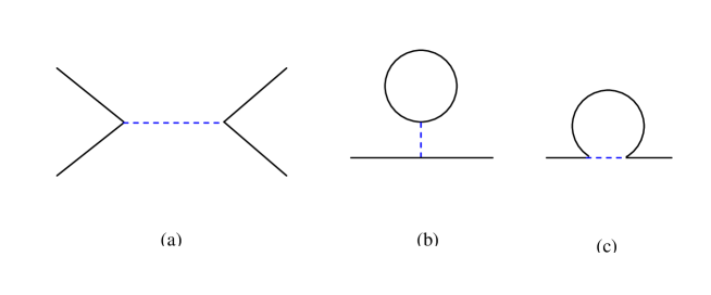
Above two dimensions, and one can redo the same type of perturbative calculation to determine the coupling renormalization. The relevant diagrams are shown in Fig. 4. One finds for the effective coupling , i.e. the coupling which includes the leading radiative correction (using dimensional regularization, which is more convenient than an explicit ultraviolet cutoff for performing actual perturbative calculations),
| (203) |
The requirement that the dimensionful effective coupling be defined independently of the scale is expressed as , and gives for the Callan-Symanzik -function (Callan, 1970; Symanzik, 1970) for
| (204) |
The above -function determines the scale dependence (at least in perturbation theory) of for an arbitrary scale, which from now on will be denoted as . Then the differential equation uniquely determines how flows as a function of momentum scale . The scale dependence of is such that if the initial is less than the ultraviolet fixed point value , with
| (205) |
then the coupling will flow towards the Gaussian fixed point at . The new phase that appears when and corresponds to a low temperature, spontaneously broken phase with finite order parameter. On the other hand if then the coupling flows towards increasingly strong coupling, and eventually out of reach of perturbation theory. In two dimensions the -function has no zero and only the strong coupling phase is present.
The one-loop running of as a function of a sliding momentum scale and can be obtained by integrating Eq. (204). One finds
| (206) |
with a positive constant and a mass scale; the combination is just the integration constant for the differential equation, which we prefer to split here in a momentum scale and a dimensionless coefficient for reasons that will become clear later. The choice of or sign is determined from whether one is to the left (+), or to right (-) of , in which case decreases or, respectively, increases as one flows away from the ultraviolet fixed point. The renormalization group invariant mass scale arises here as an arbitrary integration constant of the renormalization group equations, and cannot be determined from perturbative arguments alone. It should also be clear that multiplying both sides of Eq. (206) by the ultraviolet cutoff factor to get back the original dimensionful coupling multiplying the action in Eq. (LABEL:eq:sigma-cont) does not change any of the conclusions.
Note that the result of Eq. (206) is quite different from the naive expectation based on straight perturbation theory in dimensions (where the theory is not perturbatively renormalizable)
| (207) |
which gives a much worse ultraviolet behavior. The existence of a non-trivial ultraviolet fixed point alters the naive picture and drastically improves the ultraviolet behavior.
For large one can easily see, for example from the structure of the lattice action in Eq. (LABEL:eq:sigma-lattice), that correlation functions must decay exponentially at large separations. In the strong coupling limit, spins separated by a distance will fluctuate in an uncorrelated fashion, unless they are connected by a minimal number of link contributions from the action. One expects therefore for the lattice connected correlation function of two fields, separated by a lattice distance ,
| (208) |
which can be re-written in continuum language
| (209) |
with and . From the requirement that the correlation length be a physical quantity independent of scale, and consequently a renormalization group invariant,
| (210) |
one obtains in the strong coupling limit
| (211) |
If in Eq. (206) one sets the momentum scale equal to the cutoff scale and solves for in the strong coupling phase one obtains
| (212) |
and therefore for in terms of the bare coupling
| (213) |
This last result shows the following important fact: if is identified with the inverse of the correlation length (which can be extracted non-perturbatively, for example from the exponential decay of correlation functions, and is therefore generally unambiguous), then the calculable constant relating to in Eq. (213) uniquely determines the coefficient in Eq. (206). For example, in the large limit the value for will be given later in Eq. (244).
In general one can write down the complete renormalization group equations for the cutoff-dependent -point functions (Brezin and Zinn-Justin, 1976; Zinn-Justin, 2002). For this purpose one needs to define the renormalized truncated -point function ,
| (214) |
where is a renormalization scale, and the constants , and are defined by
| (215) |
The requirement that the renormalized -point function be independent of the cutoff then implies
| (216) |
with the renormalization group functions , and defined as
| (217) |
Here the derivatives of the bare coupling , of the -field wave function renormalization constant and of the external field with respect to the cutoff are evaluated at fixed renormalized (or effective) coupling, at the renormalization scale .
To determine the renormalization group functions , and one can in fact follow a related but equivalent procedure, in which, instead of requiring the renormalized -point functions to be independent of the cutoff at fixed renormalization scale as in Eq. (217), one imposes that the bare -point functions be independent of the renormalization scale at fixed cutoff . One can show (Brezin, Le Guillou and Zinn-Justin, 1978) that the resulting renormalization group functions are identical to the previous ones, and that one can obtain the scale dependence of the couplings (i.e. ) either way. Physically the latter way of thinking is perhaps more suited to a situation where one is dealing with a finite cutoff theory, where the ultraviolet cutoff is fixed and one wants to investigate the scale (momentum) dependence of the couplings, for example .
For our purposes it will sufficient to look, in the zero-field case , at the -function of Eq. (204) which incorporates, as should already be clear from the result of Eq. (217), a tremendous amount of information about the model. Herein lies the power of the renormalization group: the knowledge of a handful of functions [] is sufficient to completely determine the momentum dependence of all -point functions .
One can integrate the -function equation in Eq. (204) to obtain the renormalization group invariant quantity
| (218) |
which is identified with the correlation length appearing, for example, in Eq. (209). The multiplicative constant in front of the expression on the right hand side arises as an integration constant, and cannot be determined from perturbation theory in . Conversely, it is easy to verify that is indeed a renormalization group invariant, , as stated previously in Eq. (210).
In the vicinity of the fixed point at one can do the integral in Eq. (218), using Eq. (205) and the resulting linearized expression for the -function in the vicinity of the non-trivial ultraviolet fixed point,
| (219) |
and one finds
| (220) |
with a correlation length exponent . Thus the correlation length diverges as one approaches the fixed point at .
In general the existence of a non-trivial ultraviolet fixed point implies that the large momentum behavior above two dimensions is not given by naive perturbation theory; it is given instead by the critical behavior of the renormalized theory. In the weak coupling, small phase the scale can be regarded as a crossover scale between the free field behavior at large distance scales and the critical behavior which sets in at large momenta.
In the non-linear -model another quantity of physical interest is the function ,
| (221) |
which is proportional to the order parameter (the magnetization) of the non-linear -model. To one-loop order one finds and therefore
| (222) |
with and . To leading order in the expansion one has for the anomalous dimension of the field . In gauge theories, including gravity, there is no local order parameter, so this quantity has no obvious generalization there.
In general the -expansion is only expected to be asymptotic. This is already seen from the expansion for which has recently been computed to four loops (Hikami and Brezin 1978, Bernreuther and Wegner 1986, Kleinert 2000)
| (223) | |||||
which needs to be summed by Borel-Padé methods to obtain reliable results in three dimensions. For example, for one finds in three dimensions , which can be compared to the result for the theory to five loops , to the seven-loop perturbative expansion for the theory directly in which gives , with the high temperature series result and the Monte Carlo estimates , as compiled for example in a recent comprehensive review (Guida and Zinn-Justin, 1997).
There exist standard methods to deal with asymptotic series such as the one in Eq. (223). To this purpose one considers a general series
| (224) |
and defines its Borel transform as
| (225) |
One can attempt to sum the series for using Padé methods and conformal transformations. The original function is then recovered by performing an integral over the Borel transform variable
| (226) |
where the familiar formula
| (227) |
has been used. Bounds on the coefficients suggest that in most cases is analytic in a circle of radius around the origin, and that the integral will converge for small enough, within a sector with typically (Le Guillou and Zinn-Justin, 1990).
The first singularity along the positive real axis is generally referred to as an infrared renormalon, and is expected to be, in the non-linear -model, at where , and gives rise to non-analytic corrections of order (David, 1982). Such non-analytic contributions presumably account for the fact (Cardy and Hamber, 1980) that the model has a vanishing -function to all orders in , and yet has non-trivial finite exponents in , in spite of the result of Eq. (223). Indeed the expansion is not particularly useful for the special case of the -model. Then the action is simply given by
| (228) |
with and , describing the fluctuations of a planar spin in dimensions. The -function of Eq. (204) then vanishes identically in , and the corrections to diverge for , as in Eq. (223)). Yet this appears to be more a pathology of the perturbative expansion in , since after all the lattice model of Eq. (LABEL:eq:sigma-lattice) is still well defined, and so is the expansion for the continuum linear -model. Thus, in spite of the model being again not perturbatively renormalizable in , one can still develop, for these models, the full machinery of the renormalization group and compute the relevant critical exponents.
Perhaps more importantly, a recent space shuttle experiment (Lipa et al 2003) has succeeded in measuring the specific heat exponent of superfluid Helium (which is supposed to share the same universality class as the non-linear -model, with the complex phase of the superfluid condensate acting as the order parameter) to very high accuracy
| (229) |
Previous theoretical predictions for the model include the most recent four-loop continuum result (Kleinert, 2000), a recent lattice Monte Carlo estimate (Campostrini et al, 2001), and the lattice variational renormalization group prediction (Hamber, 1981).
Perhaps the message one gains from this rather lengthy discussion of the non-linear -model in is that:
-
The model provides a specific example of a theory which is not perturbatively renormalizable in the traditional sense, and for which the naive perturbative expansion in fixed dimension leads to uncontrollable divergences and inconsistent results;
-
Yet the model can be constructed perturbatively in terms of a double expansion in and . This new perturbative expansion, combined with the renormalization group, in the end provides explicit and detailed information about universal scaling properties of the theory in the vicinity of the non-trivial ultraviolet point at ;
-
The continuum field theory predictions obtained this way generally agree, for distances much larger than the cutoff scale, with lattice results, and, perhaps more importantly, with high precision experiments on systems belonging to the same universality class of the model.
II.3.2 Non-linear Sigma Model in the Large-N Limit
A rather fortunate circumstance is represented by the fact that in the large limit the non-linear -model can be solved exactly. This allows an independent verification of the correctness of the general ideas developed in the previous section, as well as a direct comparison of explicit results for universal quantities. The starting point is the functional integral of Eq. (LABEL:eq:sigma-cont),
| (230) |
with
| (231) |
The constraint on the field can be implemented via an auxiliary Lagrange multiplier field . One writes
| (232) |
with
| (233) |
Since the action is now quadratic in one can integrate over -fields (denoted previously by ). The resulting determinant is then re-exponentiated, and one is left with a functional integral over the remaining first field , as well as the Lagrange multiplier field ,
| (234) |
with now
| (235) | |||||
In the large limit one can neglect, to leading order, fluctuations in the and fields. For a constant field, , the last (trace) term can be written in momentum space as
| (236) |
which makes the evaluation of the trace straightforward. As should be clear from Eq. (233), the parameter can be interpreted as the mass of the field. The functional integral in Eq. (234) can then be evaluated by the saddle point method. It is easy to see from Eq. (235) that the saddle point conditions are
| (237) |
with the function given by the integral
| (238) |
The latter can be evaluated in terms of a hypergeometric function,
| (239) |
but here one only really needs it in the large cutoff limit, , in which case one finds the more tractable expression
| (240) |
with and some -dependent coefficients.
From Eq. (237) one notices that at weak coupling and for a non-vanishing -field expectation value implies that , the mass of the field, is zero. If one sets , one can then write the first expression in Eq. (237) as
| (241) |
which shows that is the critical coupling at which the order parameter vanishes.
Above the order parameter vanishes, and is obtained, from Eq. (237), by the solution of the nonlinear gap equation
| (242) |
Using the definition of the critical coupling , one can now write, for , for the common mass of the and fields
| (243) |
which gives for the correlation length exponent the non-gaussian value , with the gaussian value being recovered as expected at (Wilson and Fisher 1972). Note that in the large limit the constant of proportionality in Eq. (243) is completely determined by the explicit expression for .
Perhaps one of the most striking aspects of the non-linear sigma model above two dimensions is that all particles are massless in perturbation theory, yet they all become massive in the strong coupling phase , with masses proportional to the non-perturbative scale .
Again one can perform a renormalization group analysis as was done in the previous section in the context of the expansion. To this end one defines dimensionless coupling constants and as was done in Eq. (LABEL:eq:sigma-cont). Then the non-perturbative result of Eq. (243) becomes
| (244) |
with the numerical coefficient given by . One welcome feature of this large- result is the fact that it provides an explicit value for the coefficient in Eq. (213), namely
| (245) |
and thereby for the numerical factor appearing in Eqs. (213) and (206).
Again the physical, dimensionful mass in Eqs. (243) or (244) is required to be scale- and cutoff-independent as in Eq. (210)
| (246) |
or, more explicitly, using the expression for in Eq. (244),
| (247) |
which implies for the -function in the large limit the simple result
| (248) |
The latter is valid again in the vicinity of the fixed point at , due to the assumption, used in Eq. (243), of . Note that it vanishes in , and for , in agreement with the result of Eq. (204). Furthermore Eq. (248) gives the momentum dependence of the coupling at fixed cutoff. After integration, one finds for the momentum () dependence of the coupling at fixed cutoff
| (249) |
with the integration constant. The sign of then depends on whether one is on the right () or on the left () of the ultraviolet fixed point at .
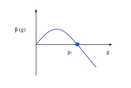
One notices therefore again that the general shape of is of the type shown in Fig. 5, with a stable non-trivial UV fixed point, and and two stable (trivial) IR fixed points. Once more, at the critical point the -function vanishes and the theory becomes scale invariant. Furthermore one can check that again where is the exponent in Eq. (243). As before one can can re-write the physical mass for as
| (250) |
as was done previously in Eq. (218).
Another general lesson one learns is that that Eq. (246),
| (251) |
can be used to provide a non-perturbative definition for the -function . If one sets , with a dimensionless function of , then one has the simple result
| (252) |
Thus the knowlegde of the dependence of the mass gap on the bare coupling fixes the shape of the function, at least in the vicinity of the fixed point. It should be clear then that the definition of the -function per se, and therefore the scale dependence of which follows from it [as determined from the solution of the differential equation ] is not necessarily tied to perturbation theory.
When is large but finite, one can develop a systematic expansion in order to evaluate the corrections to the picture presented above (Zinn-Justin, 2002). Corrections to the exponents are known up to order , but the expressions are rather complicated for arbitrary and will not be reproduced here. In general it appears that the expansion is only asymptotic, and somewhat slowly convergent for useful values of in three dimensions.
II.3.3 Self-coupled Fermion Model
Finally it would seem worthwhile to mention another example of a theory which naively is not perturbatively renormalizable in , and yet whose critical properties can be worked out both in the expansion, and in the large limit. It is described by an -invariant action containing a set of massless self-coupled Dirac fermions (Wilson, 1973; Gross and Neveu, 1974)
| (253) |
In even dimensions the discrete chiral symmetry , prevents the appearance of a fermion mass term. Interest in the model resides in the fact that it exhibits a mechanism for dynamical mass generation and chiral symmetry breaking.
In two dimensions the fermion self-coupling constant is dimensionless, and after setting one is again ready to develop the full machinery of the perturbative expansion in and , as was done for the non-linear -model, since the model is again believed to be multiplicatively renormalizable in the framework of the expansion. For the -function one finds to three loops
| (254) |
with the parameter , where the last quantity is the identity matrix in the -matrix algebra. In two dimensions and the model is asymptotically free; for the interaction is proportional to the Thirring one and the function vanishes identically.
As for the case of the non-linear -model, the solution of the renormalization group equations involves an invariant scale, which can be obtained (up to a constant which cannot be determined from perturbation theory alone) by integrating Eq. (254)
| (255) |
In two dimensions this scale is, to lowest order in , proportional to
| (256) |
and thus non-analytic in the bare coupling . Above two dimensions a non-trivial ultraviolet fixed point appears at
| (257) |
In the weak coupling phase the fermions stay massless and chiral symmetry is unbroken, whereas in the strong coupling phase (which is the only phase present in ) chiral symmetry is broken, a fermion condensate arises and a non-perturbative fermion mass is generated. In the vicinity of the ultraviolet fixed point one has for the mass gap
| (258) |
up to a constant of proportionality, with the exponent given by
| (259) |
The rest of the analysis proceeds in a way that, at least formally, is virtually identical to the non-linear -model case. It need not be repeated here, as one can just take over the relevant formulas for the renormalization group behavior of -point functions, for the running of the couplings etc.
The existence of a non-trivial ultraviolet fixed point implies that the large momentum behavior above two dimensions is not given by naive perturbation theory; it is given instead by the critical behavior of the renormalized theory, in accordance with Eq. (254). In the weak coupling, small phase the scale can be regarded as a crossover scale between the free field behavior at large distance scales and the critical behavior which sets in at large momenta.
Finally, the same model can be solved exactly in the large limit. There too one can show that the model is characterized by two phases, a weak coupling phase where the fermions are massless and a strong coupling phase in which a chiral symmetry is spontaneously broken.
II.3.4 The Gravitational Case
In two dimensions the gravitational coupling becomes dimensionless, , and the theory appears perturbatively renormalizable. In spite of the fact that the gravitational action reduces to a topological invariant in two dimensions, it would seem meaningful to try to construct, in analogy to what was suggested originally for scalar field theories (Wilson, 1973), the theory perturbatively as a double series in and .
One first notices though that in pure Einstein gravity, with Lagrangian density
| (260) |
the bare coupling can be completely reabsorbed by a field redefinition
| (261) |
with is a constant, and thus the renormalization properties of have no physical meaning for this theory. This simply follows from the fact that is homogeneous in , which is quite different from the Yang-Mills case. The situation changes though when one introduces a second dimensionful quantity to compare to. In the pure gravity case this contribution is naturally supplied by the cosmological constant term proportional to ,
| (262) |
Under a rescaling of the metric as in Eq. (261) one has
| (263) |
which is interpreted as a rescaling of the two bare couplings
| (264) |
leaving the dimensionless combination unchanged. Therefore only the latter combination has physical meaning in pure gravity. In particular, one can always choose the scale so as to adjust the volume term to have a unit coefficient. More importantly, it is physically meaningless to discuss separately the renormalization properties of and , as they are individually gauge-dependent in the sense just illustrated. These arguments should clarify why in the following it will be sufficient at the end to just focus on the renormalization properties of one coupling, such as Newton’s constant .
In general it is possible at least in principle to define quantum gravity in any . There are independent components of the metric in dimensions, and the same number of algebraically independent components of the Ricci tensor appearing in the field equations. The contracted Bianchi identities reduce the count by , and so does general coordinate invariance, leaving physical gravitational degrees of freedom in dimensions. At the same time, four space-time dimensions is known to be the lowest dimension for which Ricci flatness does not imply the vanishing of the gravitational field, , and therefore the first dimension to allow for gravitational waves and their quantum counterparts, gravitons.
In a general dimension the position space tree-level graviton propagator of the linearized theory, given in -space in Eq. (62), can be obtained by Fourier transform and is proportional to
| (265) |
The static gravitational potential is then proportional to the spatial Fourier transform
| (266) |
and can be shown to vanish in . To show this one needs to compute the analog of Eq. (17) in dimensions, which is
where the Green’s function is the static limit of , and . The above result then shows that there are no Newtonian forces in =2+1 dimensions (Deser, Jackiw and ’t Hooft, 1984; Deser and Jackiw, 1984). The only fluctuations left in are associated with the scalar curvature (Deser, Jackiw and Templeton, 1982).
The expansion for pure gravity then proceeds as follows. First the gravitational part of the action
| (267) |
with dimensionless and an arbitrary momentum scale, is expanded by setting
| (268) |
where is the classical background field and the small quantum fluctuation. The quantity in Eq. (267) is naturally identified with the bare Lagrangian, and the scale with a microscopic ultraviolet cutoff , the inverse lattice spacing in a lattice formulation. Since the resulting perturbative expansion is generally reduced to the evaluation of Gaussian integrals, the original constraint (in the Euclidean theory)
| (269) |
is no longer enforced (the same is not true in the lattice regulated theory, where it plays an important role, see the discussion following Eq. (398)).
A gauge fixing term needs to be added, in the form of a background harmonic gauge condition,
| (270) |
with , and the covariant derivative with respect to the background metric . The gauge fixing term also gives rise to a Faddeev-Popov ghost contribution containing the ghost field , so that the total Lagrangian becomes .
In a flat background, , one obtains from the quadratic part of the Lagrangian of Eqs. (267) and (270) the following expression for the graviton propagator
| (271) | |||||
Normally it would be convenient to choose a gauge =, in which case only the first two terms for the graviton propagator survive. But here it might be advantageous to leave the two gauge parameters unspecified, so that one can later show explicitly the gauge independence of the final result. In particular the gauge parameter is related to the gauge freedom associated with the possibility, described above, of rescaling the metric . Note also the presence of kinematical poles in in the second, fourth and fifth term for the graviton propagator.
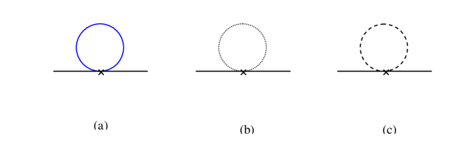
To illustrate explicitly the mechanism of coupling renormalization, the cosmological term will be discussed first, since the procedure is a bit simpler. The cosmological term is first expanded by setting with a flat background . One has
| (272) |
with . Terms linear in the fluctuation are dropped, since in a properly chosen background such terms are expected to be absent. The one-loop correction to the term in the above expression is then given by the tadpole diagrams for the two quadratic terms,
| (273) |
These are easily evaluated using the graviton propagator of Eq. (271). For the one loop divergences (see Fig. 6) associated with the term one then obtains
| (274) |
with coefficients
| (275) |
One notices that the kinematic singularities in the graviton propagator, proportional to , can combine with the one loop ultraviolet divergent part of momentum integrals, as in
| (276) |
to give terms of order in Eq. (274). Generally it is better to separate the ultraviolet divergence from the infrared one, by using for example the following regulated integral
| (277) |
for and .
One can then follow the same procedure for the term. First one needs to expand the Einstein term to quadratic order in the quantum field
where denotes the covariant derivative with respect to the background metric . The complete expansion was given previously in Eq. (LABEL:eq:h-background). The same expansion then needs to be done for the gauge fixing term of Eq. (270) as well, and furthermore it is again convenient to choose as a background field the flat metric . For the one loop divergences associated with the term one then finds
| (279) |
with the coefficient given by (Gastmans et al 1977, Christensen et al 1978)
| (280) |
Thus the one-loop radiative corrections modify the total Lagrangian to
| (281) |
Next one can make use of the freedom to rescale the metric, by setting
| (282) |
which restores the original unit coefficient for the cosmological constant term. The rescaling is achieved by the following field redefinition
| (283) |
Hence the cosmological term is brought back into the standard form , and one obtains for the complete Lagrangian to first order in
| (284) |
where only terms singular in have been retained. From this last result one can finally read off the renormalization of Newton’s constant
| (285) |
From Eqs. (275) and (280) one notices that the contribution cancels out the gauge-dependent part of , giving for the remaining contribution . Therefore the gauge dependence has, as one would have hoped on physical grounds, disappeared from the final answer. It is easy to see that the same result would have been obtained if the scaled cosmological constant had been held constant, instead of as in Eq. (282). One important aspect of the result of Eq. (285) is that the quantum correction is negative, meaning that the strength of is effectively increased by the lowest order radiative correction.
In the presence of an explicit renormalization scale parameter the -function for pure gravity is obtained by requiring the independence of the quantity (here identified as an effective coupling constant, with lowest order radiative corrections included) from the original renormalization scale ,
| (286) |
To zero-th order in , the renormalization group -function entering the renormalization group equation
| (287) |
is just given by
| (288) |
The above result just follows from the trivial scale dependence of the classical, dimensionful gravitational coupling: to achieve a fixed given , the dimensionless quantity itself has to scale like . Next, to first order in , one has from Eq. (286)
| (289) |
with . From the procedure outlined above it is clear that is the only coupling that is scale-dependent in pure gravity. As will be appreciated further below, the importance of the gravitational -function lies in the fact that it can be used either to determine the ultraviolet cutoff dependence of the bare coupling needed to keep the effective coupling fixed (as in Eq. (286), or to determine the momentum dependence of the physical coupling for a fixed cutoff.
Matter fields can be included as well. When scalar fields and Majorana fermion fields are added, the results of Eqs. (280), (285) and (286) are modified to
| (290) |
with (the central charge of the Virasoro algebra in two dimensions), and therefore for the combined -function of Eq. (289) to one-loop order one has . Of course one noteworthy aspect of the perturbative calculation is the appearance of a non-trivial ultraviolet fixed point at for which , whose physical significance will be discussed further below.
To check their consistency, the above one-loop calculations have been repeated by performing a number of natural variations. One modification consists in using the Thirring interaction
| (291) |
instead of the cosmological constant term to set the scale for the metric. This results in a -function still of the form of Eq. (289) but with . The slight discrepancy between the two results was initially attributed (Kawai and Ninomiya, 1990) to the well known problems related to the kinematic singularities of the graviton propagator in discussed previously. To address this issue, a new perturbative expansion can be performed with the metric parametrized as
| (292) |
where the conformal mode (responsible for the kinematic singularity in the second term on the r.h.s. of Eq. (271)) is explicitly separated out, and is now taken to be traceless, . Furthermore the conformal mode is made massive by adding a cosmological constant term , which again acts as an infrared regulator. Repeating the calculation for the one loop divergences (Kawai, Kitazawa and Ninomiya, 1993) one now finds which is consistent with the above quoted Thirring result 555 For a while there was considerable uncertainty about the magnitude of the graviton contribution to , which was quoted originally as (Tsao 1977), later as (Gastman et al 1977, Christensen and Duff 1978; Weinberg, 1977), and more recently as (Kawai, Kitazawa and Ninomiya, 1992). As discussed in (Weinberg, 1977), the original expectation was that the graviton contribution should be times the scalar contribution close to , which would suggest for gravity the value . Direct numerical estimates of the scaling exponent in the lattice theory for (Hamber and Williams, 1993) give, using Eq. (306), a value and are therefore in much better agreement with the larger, more recent values..
In the meantime the calculations have been laboriously extended to two loops (Aida and Kitazawa, 1997), with the result
| (293) |
with and .
II.3.5 Phases of Gravity in Dimensions
The gravitational -function of Eqs. (289) and (293) determines the scale dependence of Newton’s constant for close to two. It has the general shape shown in Fig. 7. Because one is left, for the reasons described above, with a single coupling constant in the pure gravity case, the discussion becomes in fact quite similar to the non-linear -model case.
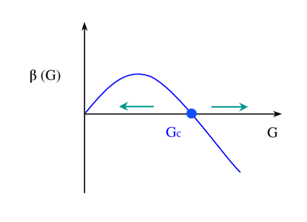
For a qualitative discussion of the physics it will be simpler in the following to just focus on the one loop result of Eq. (289); the inclusion of the two-loop correction does not alter the qualitative conclusions by much, as it has the same sign as the lower order, one-loop term. Depending on whether one is on the right () or on the left () of the non-trivial ultraviolet fixed point at
| (294) |
(with positive provided one has ) the coupling will either flow to increasingly larger values of , or flow towards the Gaussian fixed point at , respectively. In the following we will refer to the two phases as the strong coupling and weak coupling phase, respectively. Perturbatively one only has control on the small regime. When one then sets only the strong coupling phase survives, so two-dimensional gravity is always strongly coupled within this picture.
The running of as a function of a sliding momentum scale in pure gravity can be obtained by integrating Eq. (289), and one finds
| (295) |
with a positive constant and a mass scale. The choice of or sign is determined from whether one is to the left (+), or to right (-) of , in which case the effective decreases or, respectively, increases as one flows away from the ultraviolet fixed point towards lower momenta, or larger distances. Physically the two solutions represent a screening () and an anti-screening () situation. The renormalization group invariant mass scale arises here as an arbitrary integration constant of the renormalization group equations (one could have absorbed the constant in , but we will not do so here for reasons that will become clearer later).
While in the continuum perturbative calculation both phases, and therefore both signs, seem acceptable, the Euclidean lattice results on the other hand seem to rule out the weak coupling phase as pathological, in the sense that the lattice collapses into a two-dimensional branched polymer, as will be discussed later in this review in Sec. IV.1.
At the opposite end, at energies sufficiently high to become comparable to the ultraviolet cutoff (the inverse lattice spacing in a lattice discretization), the gravitational coupling flows towards the ultraviolet fixed point,
| (296) |
where is the coupling at the cutoff scale , to be identified with the bare (or lattice) coupling. Note that it would seem meaningless to consider, within this framework, momenta which are larger than the ultraviolet cutoff . At such energies higher dimension operators (such as higher derivative curvature terms) are expected to become important and should therefore be included in the microscopic action.
Note that the result of Eq. (295) is quite different from the naive expectation based on straight perturbation theory in dimensions (where the theory is not perturbatively renormalizable)
| (297) |
which gives a much worse ultraviolet behavior. The existence of a non-trivial ultraviolet fixed point alters the naive picture and drastically improves the ultraviolet behavior.
The -dependent contribution in the denominator of Eq. (295) is the quantum correction, which at least within a perturbative framework is assumed to be small. In the weak coupling phase the coupling then flows towards the origin corresponding to a gravitational screening solution, which sounds a bit odd as one would not expect gravity to be screened. On the other hand the infrared growth of the coupling in the strong coupling phase can be written equivalently as
| (298) |
where the dots indicate higher order radiative corrections, and which exhibits a number of interesting features. Firstly the fractional power suggests new non-trivial gravitational scaling dimensions, just as in the case of the non-linear -model. Furthermore, the quantum correction involves a new physical, renormalization group invariant scale which cannot be fixed perturbatively, and whose size determines the scale for the quantum effects. In terms of the bare coupling , it is given by
| (299) |
which just follows from integrating and then setting as the arbitrary scale . Conversely, since is an invariant, one has ; the running of in accordance with the renormalization group equation of Eq. (287) ensures that the l.h.s. is indeed a renormalization group invariant. The constant on the r.h.s. of Eq. (299) cannot be determined perturbatively, it needs to be computed by non-perturbative (lattice) methods, for example by evaluating invariant correlations at fixed geodesic distances. It is related to the constant in Eq. (298) by .
At the fixed point the theory is scale invariant by definition. In statistical field theory language the fixed point corresponds to a phase transition, where the correlation length diverges and the theory becomes scale (conformally) invariant. In general in the vicinity of the fixed point, for which , one can write
| (300) |
If one then defines the exponent by
| (301) |
then from Eq. (299) one has by integration in the vicinity of the fixed point
| (302) |
which is why is often referred to as the mass gap exponent. Solving the above equation (with ) for one obtains back Eq. (298), with the constant there related to in Eq. (302) by and .
That is a renormalization group invariant is seen from
| (303) |
provided runs in accordance with Eq. (298). To one-loop order one has from Eqs. (289) and (301) . When the bare (lattice) coupling one has achieved criticality, . How far the bare theory is from the critical point is determined by the choice of , the distance from criticality being measured by the deviation .
Furthermore Eq. (302) shows how the (lattice) continuum limit is to be taken. In order to reach the continuum limit for fixed physical correlation , the bare coupling needs to be tuned so as to approach the ultraviolet fixed point at ,
| (304) |
The fixed point at thus plays a central role in the cutoff theory: together with the universal scaling exponent it determines the correct unique quantum continuum limit in the presence of an ultraviolet cutoff . Sometimes it can be convenient to measure all quantities in units of the cutoff and set . In this case the quantity measured in units of the cutoff (i.e. ) has to be tuned to zero in order to construct the lattice continuum limit: for a fixed lattice cutoff, the continuum limit is approached by tuning the bare lattice to . In other words, the lattice continuum limit has to be taken in the vicinity of the non-trivial ultraviolet point.
The discussion given above is not altered significantly, at least in its qualitative aspects, by the inclusion of the two-loop correction of Eq. (293). From the expression for the two-loop -function
| (305) |
for massless real scalar fields minimally coupled to gravity, one computes the roots to obtain the location of the ultraviolet fixed point, and from it on can then determine the universal exponent . One finds
| (306) |
which gives, for pure gravity without matter () in four dimensions, to lowest order , and at the next order.
Also, in general higher order corrections to the results of the linearized renormalization group equations of Eq. (300) are present, which affect the scaling away from the fixed point. Let us assume that close to the ultraviolet fixed point at one can write for the -function the following expansion
| (307) |
After integrating as before, one finds for the structure of the correction to [see for comparison Eq. (302)]
| (308) |
The hope of course is that these corrections to scaling are small, ; in the vicinity of the fixed point the higher order term becomes unimportant when . For the effective running coupling one then has
| (309) |
which gives an estimate for the size of the modifications to Eq. (298).
Finally, as a word of caution, one should mention that in general the convergence properties of the expansion are not well understood. The poor convergence found in some better known cases is usually ascribed to the suspected existence of infrared renormalon-type singularities close to two dimensions, and which could possibly arise in gravity as well. At the quantitative level, the results of the expansion for gravity therefore remain somewhat limited, and obtaining the three- or four-loop term still represents a daunting task. Nevertheless they provide, through Eqs. (298) and (302), an analytical insight into the scaling properties of quantum gravity close and above two dimensions, including the suggestion of a non-trivial phase structure and an estimate for the non-trivial universal scaling exponents (Eq. (306)). The key question raised by the perturbative calculations is therefore: what remains of the above phase transition in four dimensions, how are the two phases of gravity characterized there non-perturbatively, and what is the value of the exponent determining the running of in the vicinity of the fixed point in four dimensions.
Finally we should mention that there are other continuum renormalization group methods which can be used to estimate the scaling exponents. An approach which is closely related to the expansion for gravity is the derivation of approximate flow equations from the changes of the Legendre effective action with respect to a suitably introduced infrared cutoff . The method can be regarded as a variation on Wilson’s original momentum slicing technique for obtaining approximate renormalization group equations for lattice couplings. In the simplest case of a scalar field theory (Morris, 1994) one starts from the partition function
| (310) |
The term is taken to be an ’additive infrared cutoff term’. For it to be an infrared cutoff it needs to be small for , ideally tending to zero as , and such that is large when . Since the method is only ultimately applied to the vicinity of the fixed point, for which all physical relevant scales are much smaller than the ultraviolet cutoff , it is argued that the specific nature of this cutoff is not really relevant in the following. Taking a derivative of with respect to the scale gives
| (311) |
which can be re-written in terms of the Legendre transform as
| (312) |
where now is regarded as the classical field. The traces can then be simplified by writing them in momentum space. What remains to be done is first settle on a suitable cutoff function , and subsequently compute the effective action in a derivative expansion, thus involving terms of the type , with dependent coefficients.
As far as the cutoff function is concerned, it is first written as so as to include the expected anomalous dimensions of the propagator. To simplify things further, it is then assumed for the remaining function of a single variables that with a non-negative integer (Morris, 1994). The subsequent derivative expansion gives for example for the model in to lowest order an anomalous dimensions for all , and for . At the next order in the derivative expansion the method gives , compared to the best theoretical and experimental value (Morris and Turner 1997).
In the gravitational case one can proceed in a similar way. First the gravity analog of Eq. (312) is clearly
| (313) |
where now corresponds to the classical metric. The effective action itself contains the Einstein and cosmological terms
| (314) |
as well as gauge fixing and possibly higher derivative terms (Reuter 1998). After the addition of a background harmonic gauge fixing term with gauge parameter , the choice of a suitable (scalar) cutoff function is required, (Litim 2004), which is inserted into
| (315) |
Note that this added momentum-dependent cutoff term violates both the weak field general coordinate invariance [see for instance Eq. (11)], as well as the general rescaling invariance of Eq. (263).
The solution of the resulting renormalization group equation for the two couplings and is then truncated to the Einstein and cosmological term, a procedure which is equivalent to the derivative expansion discussed previously. A nontrivial fixed point in both couplings () is then found in four dimensions, with complex eigenvalues for a gauge parameter choice [for general gauge parameter the exponents can vary by as much as seventy percent (Lauscher and Reuter 2002)]. In the special limit of vanishing cosmological constant the equations simplify further and one finds a trivial Gaussian fixed point at , as well as a non-trivial ultraviolet fixed point with , which in gives now . So in spite of the apparent crudeness of the lowest order approximation, an ultraviolet fixed point similar to the one found in the expansion is recovered.
II.3.6 Running of in and
and provide two invaluable illustrative cases where the running of the gauge coupling with energy is not only theoretically well understood, but also verified experimentally. This section is intended to provide analogies and distinctions between the two theories, in a way later suitable for a comparison with the gravitational case. Most of the results found in this section are well known (see, for example, Frampton, 2000), but the purpose here is to provide some contrast (and in some instances, a relationship) with the gravitational case.
In the non-relativistic static Coulomb potential is affected by the vacuum polarization contribution due to electrons (and positrons) of mass . To lowest order in the fine structure constant, the contribution is from a single Feynman diagram involving a fermion loop. One finds for the vacuum polarization contribution at small the well known result (Itzykson and Zuber, 1980)
| (316) |
which, for a Coulomb potential with a charge centered at the origin of strength leads to well-known Uehling -function correction
| (317) |
It is not necessary though to resort to the small- approximation, and in general a static charge of strength at the origin will give rise to a modified potential
| (318) |
with
| (319) |
for small , and
| (320) |
for large . Here the normalization is such that the potential at infinity has 666 The running of the fine structure constant has recently been verified experimentally at . The scale dependence of the vacuum polarization effects gives a fine structure constant changing from at atomic distances to about at energies comparable to the boson mass, in good agreement with the theoretical renormalization group prediction.. The reason we have belabored this example is to show that the screening vacuum polarization contribution would have dramatic effects in QED if for some reason the particle running through the fermion loop diagram had a much smaller (or even close to zero) mass. There are two interesting aspects of the (one-loop) result of Eqs. (319) and (320). The first one is that the exponentially small size of the correction at large is linked with the fact that the electron mass is not too small: the range of the correction term is , but would have been much larger if the electron mass had been a lot smaller.
In (and related Yang-Mills theories) radiative corrections are also known to alter significantly the behavior of the static potential at short distances. The changes in the potential are best expressed in terms of the running strong coupling constant , whose scale dependence is determined by the celebrated beta function of with light fermion flavors
| (321) |
with , , and . The solution of the renormalization group equation Eq. (321) then gives for the running of
| (322) |
(see Fig. 8). The non-perturbative scale appears as an integration constant of the renormalization group equations, and is therefore - by construction - scale independent. The physical value of cannot be fixed from perturbation theory alone, and needs to be determined by experiment, giving .
In principle one can solve for in terms of the coupling at any scale, and in particular at the cutoff scale , obtaining
| (323) |
In lattice QCD this is usually taken as the definition of the running strong coupling constant . It then leads to an effective potential between quarks and anti-quarks of the form
| (324) |
and the leading logarithmic correction makes the potential appear softer close to the origin, .
When the result is contrasted with the answer of Eqs. (316) and (317) it appears that the infrared small singularity in Eqs. (324) is quite serious. An analogous conclusion is reached when examining Eqs. (322): the coupling strength diverges in the infrared due to the singularity at . In phenomenological approaches to low energy (Richardson, 1979) the uncontrolled growth in due to the spurious small- divergence is regulated by the dynamically generated infrared cutoff , which can then be shown to give a confining linear potential at large distances.
Not all physical properties can be computed reliably in weak coupling perturbation theory. In non-Abelian gauge theories a confining potential is found at strong coupling by examining the behavior of the Wilson loop (Wilson, 1973), defined for a large closed loop as
| (325) |
with and the ’s the group generators of in the fundamental representation. In the pure gauge theory at strong coupling, the leading contribution to the Wilson loop can be shown to follow an area law for sufficiently large loops
| (326) |
where is the minimal area spanned by the planar loop . The quantity is the gauge field correlation length, defined for example from the exponential decay of the Euclidean correlation function of two infinitesimal loops separated by a distance ,
| (327) |
Here the ’s are two infinitesimal loops centered around ands respectively, suitably defined on the lattice as elementary square loops, and for which one has at sufficiently large separations
| (328) |
The inverse of the correlation length corresponds to the lowest mass excitation in the gauge theory, the scalar glueball, . Notice that since the glueball mass is expected to be proportional to the parameter of Eq. (323) for small , it is non-analytic in the gauge coupling.

III LATTICE REGULARIZED QUANTUM GRAVITY
The following sections are based on the lattice discretized description of gravity known as Regge calculus, where the Einstein theory is expressed in terms of a simplicial decomposition of space-time manifolds. Its use in quantum gravity is prompted by the desire to make use of techniques developed in lattice gauge theories (Wilson, 1973) 777 As an example of a state-of-the-art calculation of hadron properties in the lattice formulation of see (Aoki et al., 2003). , but with a lattice which reflects the structure of space-time rather than just providing a flat passive background (Regge, 1961). It also allows one to use powerful nonperturbative analytical techniques of statistical mechanics as well as numerical methods. A regularized lattice version of the continuum field theory is also usually perceived as a necessary prerequisite for a rigorous study of the latter.
In Regge gravity the infinite number of degrees of freedom in the continuum is restricted by considering Riemannian spaces described by only a finite number of variables, the geodesic distances between neighboring points. Such spaces are taken to be flat almost everywhere and are called piecewise linear (Singer and Thorpe, 1967). The elementary building blocks for -dimensional space-time are simplices of dimension . A 0-simplex is a point, a 1-simplex is an edge, a 2-simplex is a triangle, a 3-simplex is a tetrahedron. A -simplex is a -dimensional object with vertices and edges connecting them. It has the important property that the values of its edge lengths specify the shape, and therefore the relative angles, uniquely.
A simplicial complex can be viewed as a set of simplices glued together in such a way that either two simplices are disjoint or they touch at a common face. The relative position of points on the lattice is thus completely specified by the incidence matrix (it tells which point is next to which) and the edge lengths, and this in turn induces a metric structure on the piecewise linear space. Finally the polyhedron constituting the union of all the simplices of dimension is called a geometrical complex or skeleton. The transition from a smooth triangulation of a sphere to the corresponding secant approximation is illustrated in Fig. 9.

A manifold can then be defined by its relationship to a piecewise linear space: a topological space is called a closed -dimensional manifold if it is homeomorphic to a connected polyhedron, and furthermore, if its points possess neighborhoods which are homeomorphic to the interior of the d-dimensional sphere.
III.1 General Formulation
We will consider here a general simplicial lattice in dimensions, made out of a collection of flat -simplices glued together at their common faces so as to constitute a triangulation of a smooth continuum manifold, such as the -torus or the surface of a sphere. If we focus on one such -simplex, it will itself contain sub-simplices of smaller dimensions; as an example in four dimensions a given 4-simplex will contain 5 tetrahedra, 10 triangles (also referred to as hinges in four dimensions), 10 edges and 5 vertices. In general, an -simplex will contain -simplices in its boundary. It will be natural in the following to label simplices by the letter , faces by and hinges by . A general connected, oriented simplicial manifold consisting of simplices will also be characterized by an incidence matrix , whose matrix element is chosen to be equal to one if the two simplices labeled by and share a common face, and zero otherwise.
The geometry of the interior of a -simplex is assumed to be flat, and is therefore completely specified by the lengths of its edges. Let be the -th coordinate of the -th site. For each pair of neighboring sites and the link length squared is given by the usual expression
| (329) |
with the flat metric. It is therefore natural to associate, within a given simplex , an edge vector with the edge connecting site to site .

III.1.1 Volumes and Angles
When focusing on one such -simplex it will be convenient to label the vertices by and denote the square edge lengths by , … , . The simplex can then be spanned by the set of vectors , … connecting the vertex to the other vertices. To the remaining edges within the simplex one then assigns vectors with . One has therefore independent vectors, but invariants given by all the edge lengths squared within .
In the interior of a given simplex one can also assign a second, orthonormal (Lorentz) frame, which we will denote in the following by . The expansion coefficients relating this orthonormal frame to the one specified by the directed edges of the simplex associated with the vectors is the lattice analog of the -bein or tetrad .
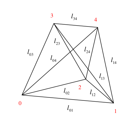
Within each -simplex one can define a metric
| (330) |
with , and which in the Euclidean case is positive definite. In components one has . In terms of the edge lengths , the metric is given by
| (331) |
Comparison with the standard expression for the invariant interval confirms that for the metric in Eq. (331) coordinates have been chosen along the directions.
The volume of a general -simplex is given by the -dimensional generalization of the well-known formula for a tetrahedron, namely
| (332) |
An equivalent, but more symmetric, form for the volume of an -simplex can be given in terms of the bordered determinant of an matrix (Wheeler, 1964)
| (333) |
It is possible to associate -forms with lower dimensional objects within a simplex, which will become useful later (Hartle, 1984). With each face of an -simplex (in the shape of a tetrahedron in four dimensions) one can associate a vector perpendicular to the face
| (334) |
where are a set of oriented edges belonging to the face , and is the sign of the permutation .
The volume of the face is then given by
| (335) |
Similarly, one can consider a hinge (a triangle in four dimensions) spanned by edges ,, . One defines the (un-normalized) hinge bivector
| (336) |
with the area of the hinge then given by
| (337) |
Next, in order to introduce curvature, one needs to define the dihedral angle between faces in an -simplex. In an -simplex two -simplices and will intersect on a common -simplex , and the dihedral angle at the specified hinge is defined as
| (338) |
where the scalar product appearing on the r.h.s. can be re-written in terms of squared edge lengths using
| (339) |
and in turn expressed in terms of squared edge lengths by the use of Eq. (331). (Note that the dihedral angle would have to be defined as minus the arccosine of the expression on the r.h.s. if the orientation for the ’s had been chosen in such a way that the ’s would all point from the face inward into the simplex ). As an example, in two dimensions and within a given triangle, two edges will intersect at a vertex, giving as the angle between the two edges. In three dimensions within a given simplex two triangles will intersect at a given edge, while in four dimension two tetrahedra will meet at a triangle. For the special case of an equilateral -simplex, one has simply . A related and often used formula for the sine of the dihedral angle is
| (340) |
but is less useful for practical calculations, as the sine of the angle does not unambiguously determine the angle itself, which is needed in order to compute the local curvature.
In a piecewise linear space curvature is detected by going around elementary loops which are dual to a ()-dimensional subspace. From the dihedral angles associated with the faces of the simplices meeting at a given hinge one can compute the deficit angle , defined as
| (341) |
where the sum extends over all simplices meeting on . It then follows that the deficit angle is a measure of the curvature at . The two-dimensional case is illustrated in Fig. 12, while the three- and four-dimensional cases are shown in Fig. 13.


III.1.2 Rotations, Parallel Transports and Voronoi Loops
Since the interior of each simplex is assumed to be flat, one can assign to it a Lorentz frame . Furthermore inside one can define a -component vector . Under a Lorentz transformation of , described by the matrix satisfying the usual relation for Lorentz transformation matrices
| (342) |
the vector will rotate to
| (343) |
The base edge vectors themselves are of course an example of such a vector.
Next consider two -simplices, individually labeled by and , sharing a common face of dimensionality . It will be convenient to label the edges residing in the common face by indices . Within the first simplex one can then assign a Lorentz frame , and similarly within the second one can assign the frame . The edge vectors on the common interface (corresponding physically to the same edges, viewed from two different coordinate systems) are expected to be related to each other by a Lorentz rotation ,
| (344) |
Under individual Lorentz rotations in and one has of course a corresponding change in , namely . In the Euclidean -dimensional case is an orthogonal matrix, element of the group .
In the absence of torsion, one can use the matrix to describes the parallel transport of any vector from simplex to a neighboring simplex ,
| (345) |
therefore describes a lattice version of the connection (Lee, 1983). Indeed in the continuum such a rotation would be described by the matrix
| (346) |
with the affine connection. The coordinate increment is interpreted as joining the center of to the center of , thereby intersecting the face . On the other hand, in terms of the Lorentz frames and defined within the two adjacent simplices, the rotation matrix is given instead by
| (347) |
(this last matrix reduces to the identity if the two orthonormal bases and are chosen to be the same, in which case the connection is simply given by ). Note that it is possible to choose coordinates so that is the unit matrix for one pair of simplices, but it will not then be unity for all other pairs.
This last set of results will be useful later when discussing lattice Fermions. Let us consider here briefly the problem of how to introduce lattice spin rotations. Given in dimensions the above rotation matrix , the spin connection between two neighboring simplices and is defined as follows. Consider to be an element of the -dimensional representation of the covering group of , , with or , and for which is a matrix of dimension . Then can be written in general as
| (348) |
where is an antisymmetric matrix The ’s are matrices, generators of the Lorentz group ( in the Euclidean case, and in the Lorentzian case), whose explicit form is
| (349) |
so that, for example,
| (350) |
For Fermions the corresponding spin rotation matrix is then obtained from
| (351) |
with generators , and with the Dirac matrices satisfying as usual . Taking appropriate traces, one can obtain a direct relationship between the original rotation matrix and the corresponding spin rotation matrix
| (352) |
which determines the spin rotation matrix up to a sign.
One can consider a sequence of rotations along an arbitrary path going through simplices , whose combined rotation matrix is given by
| (353) |
and which describes the parallel transport of an arbitrary vector from the interior of simplex to the interior of simplex ,
| (354) |
If the initial and final simplices and coincide, one obtains a closed path , for which the associated expectation value can be considered as the gravitational analog of the Wilson loop. Its combined rotation is given by
| (355) |
Under Lorentz transformations within each simplex along the path one has a pairwise cancellation of the matrices except at the endpoints, giving in the closed loop case
| (356) |
Clearly the deviation of the matrix from unity is a measure of curvature. Also, the trace is independent of the choice of Lorentz frames.
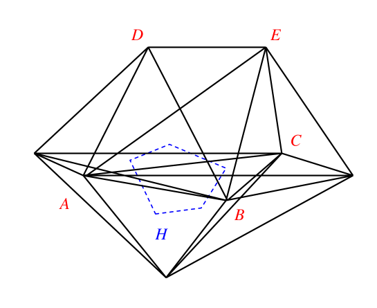
Of particular interest is the elementary loop associated with the smallest non-trivial, segmented parallel transport path one can build on the lattice. One such polygonal path in four dimensions is shown in Fig. 14. In general consider a -dimensional simplex (hinge) , which will be shared by a certain number of -simplices, sequentially labeled by , and whose common faces will also contain the hinge . Thus in four dimensions several four-simplices will contain, and therefore encircle, a given triangle (hinge). In three dimensions the path will encircle an edge, while in two dimensions it will encircle a site. Thus for each hinge there is a unique elementary closed path for which one again can define the ordered product
| (357) |
The hinge , being geometrically an object of dimension , is naturally represented by a tensor of rank , referred to a coordinate system in : an edge vector in , and an area bi-vector in etc. Following Eq. (336) it will therefore be convenient to define a hinge bi-vector in any dimension as
| (358) |
normalized, by the choice of the constant , in such a way that . In four dimensions
| (359) |
where and two independent edge vectors associated with the hinge , and the area of the hinge.
An important aspect related to the rotation of an arbitrary vector, when parallel transported around a hinge , is the fact that, due to the hinge’s intrinsic orientation, only components of the vector in the plane perpendicular to the hinge are affected. Since the direction of the hinge is specified locally by the bivector of Eq. (359), one can write for the loop rotation matrix
| (360) |
where is now the small polygonal loop entangling the hinge , and the deficit angle at , previously defined in Eq. (341). One particularly noteworthy aspect of this last result is the fact that the area of the loop does not enter in the expression for the rotation matrix, only the deficit angle and the hinge direction.
At the same time, in the continuum a vector carried around an infinitesimal loop of area will change by
| (361) |
where is an area bivector in the plane of , with squared magnitude . Since the change in the vector is given by one is led to the identification
| (362) |
Thus the above change in can equivalently be re-written in terms of the infinitesimal rotation matrix
| (363) |
(where the Riemann tensor appearing in the exponent on the r.h.s. should not be confused with the rotation matrix on the l.h.s.).
It is then immediate to see that the two expressions for the rotation matrix in Eqs. (360) and (363) will be compatible provided one uses for the Riemann tensor at a hinge the expression
| (364) |
expected to be valid in the limit of small curvatures, with the area of the loop entangling the hinge . Here use has been made of the geometric relationship . Note that the bivector has been defined to be perpendicular to the edge vectors spanning the hinge , and lies therefore in the same plane as the loop . Furthermore, the expression of Eq. (364) for the Riemann tensor at a hinge has the correct algebraic symmetry properties, such as the antisymmetry in the first and second pair of indices, as well as the swap symmetry between first and second pair, and is linear in the curvature, with the correct dimensions of one over length squared.
The area is most suitably defined by introducing the notion of a dual lattice, i.e. a lattice constructed by assigning centers to the simplices, with the polygonal curve connecting these centers sequentially, and then assigning an area to the interior of this curve. One possible way of assigning such centers is by introducing perpendicular bisectors to the faces of a simplex, and locate the vertices of the dual lattice at their common intersection, a construction originally discussed in (Voronoi, 1908) and in (Meijering, 1953). Another, and perhaps even simpler, possibility is to use a barycentric subdivision (Singer and Thorpe, 1967).
III.1.3 Invariant Lattice Action
The first step in writing down an invariant lattice action, analogous to the continuum Einstein-Hilbert action, is to find the lattice analog of the Ricci scalar. From the expression for the Riemann tensor at a hinge given in Eq. (364) one obtains by contraction
| (365) |
The continuum expression is then obtained by multiplication with the volume element associated with a hinge. The latter is defined by first joining the vertices of the polyhedron , whose vertices lie in the dual lattice, with the vertices of the hinge , and then computing its volume.
By defining the polygonal area as , where is the volume of the hinge (an area in four dimensions), one finally obtains for the Euclidean lattice action for pure gravity
| (366) |
with the constant . One would have obtained the same result for the single-hinge contribution to the lattice action if one had contracted the infinitesimal form of the rotation matrix in Eq. (360) with the hinge bivector of Eq. (336) (or equivalently with the bivector of Eq. (359) which differs from by a constant). The fact that the lattice action only involves the content of the hinge (the area of a triangle in four dimensions) is quite natural in view of the fact that the rotation matrix at a hinge in Eq. (360) only involves the deficit angle, and not the polygonal area .
An alternative form for the lattice action (Fröhlich, 1981) can be obtained instead by contracting the elementary rotation matrix of Eq. (360), and not just its infinitesimal form, with the hinge bivector of Eq. (336),
| (367) |
The above construction can be regarded as analogous to Wilson’s lattice gauge theory, for which the action also involves traces of products of color rotation matrices (Wilson, 1973). For small deficit angles one can of course use to show the equivalence of the two lattice actions.
But in general, away from a situation of small curvatures, the two lattice action are not equivalent, as can be seen already in two dimensions. Writing the rotation matrix at a hinge as , expressed for example in terms of Pauli matrices, and taking the appropriate trace ( in two dimensions) one finds
| (368) |
and therefore . In general one can show that the compact action in dimensions involves the sine of the deficit angle, instead of just the angle itself as in the Regge case. In the weak field limit the two actions should lead to similar expansions, while away from the weak field limit one would have to verify that the same universal long distance properties are recovered.
The preceding observations can in fact be developed into a consistent first order (Palatini) formulation of Regge gravity, with suitably chosen independent transformation matrices and metrics, related to each other by a set of appropriate lattice equations of motion (Caselle, d’Adda and Magnea, 1986). Ultimately one would expect the first and second order formulations to describe the same quantum theory, with common universal long-distance properties. How to consistently define finite rotations, frames and connections in Regge gravity was first discussed systematically in (Fröhlich, 1981).
One important result that should be mentioned in this context is the rigorous proof of convergence in the sense of measures of the Regge lattice action towards the continuum Einstein-Hilbert action (Cheeger, Müller and Schrader, 1984). Some general aspects of this result have recently been reviewed from a mathematical point of view in (Lafontaine, 1986). A derivation of the Regge action from its continuum counterpart was later presented in (Lee, Feinberg and Friedberg, 1984).
Other terms can be added to the lattice action. Consider for example a cosmological constant term, which in the continuum theory takes the form . The expression for the cosmological constant term on the lattice involves the total volume of the simplicial complex. This may be written as
| (369) |
or equivalently as
| (370) |
where is the volume associated with each hinge via the construction of a dual lattice, as described above. Thus one may regard the local volume element as being represented by either (centered on ) or (centered on ).
The Regge and cosmological constant term then lead to the combined action
| (371) |
One would then write for the lattice regularized version of the Euclidean Feynman path integral
| (372) |
where is an appropriate functional integration measure over the edge lengths, to be discussed later.
The structure of the gravitational action of Eq. (371) leads naturally to some rather general observations, which we will pursue here. The first, cosmological constant, term represents the total four-volume of space-time. As such, it does not contain any derivatives (or finite differences) of the metric and is completely local; it does not contribute to the propagation of gravitational degrees of freedom and is more akin to a mass term (as is already clear from the weak field expansion of in the continuum). In an ensemble in which the total four-volume is fixed in the thermodynamic limit (number of simplices tending to infinity) one might in fact take the lattice coupling , since different values of just correspond to a trivial rescaling of the overall four-volume (of course in a traditional renormalization group approach to field theory, the overall four-volume is always kept fixed while the scale or dependence of the action and couplings are investigated). Alternatively, one might even want to choose directly an ensemble for which the probability distribution in the total four-volume is
| (373) |
in analogy with the microcanonical ensemble of statistical mechanics.
The second, curvature contribution to the action contains, as in the continuum, the proper kinetic term. This should already be clear from the derivation of the lattice action given above, and will be made even more explicit in the section dedicated to the lattice weak field expansion. Such a term now provides the necessary coupling between neighboring lattice metrics, but the coupling still remains local. Geometrically, it can be described as a sum of elementary loop contributions, as it contains as its primary ingredient the deficit angle associated with an elementary parallel transport loop around the hinge . When one resides in the extreme strong coupling regime There the fluctuations in the metric are completely unconstrained by the action, insofar as only the total four-volume of the manifold is kept constant.
At this point it might be useful to examine some specific cases with regards to the overall dimensionality of the simplicial complex. In two dimensions the Regge action reduces to a sum over lattice sites of the deficit angle, giving the discrete analog of the Gauss-Bonnet theorem
| (374) |
where is the Euler characteristic of the surface, and the genus (the number of handles). In this case the action is therefore a topological invariant, and the above lattice expression is therefore completely analogous to the well known continuum result
| (375) |
This remarkable identity ensures that two-dimensional lattice -gravity is as trivial as in the continuum, since the variation of the local action density under a small variation of an edge length is still zero. Of course there is a much simpler formula for the Euler characteristic of a simplicial complex, namely
| (376) |
where is the number of simplices of dimension . Also it should be noted that in two dimensions the compact action does not satisfy the Gauss-Bonnet relation.
In three dimensions the Regge lattice action reads
| (377) |
where is the deficit angle around the edge labeled by . Variation with respect to an edge length gives two terms, of which only the term involving the variation of the edge is non-zero
| (378) |
In fact it was shown by Regge that for any the term involving the variation of the deficit angle does not contribute to the equations of motion (just as in the continuum the variation of the Ricci tensor does not contribute to the equations of motion either). Therefore in three dimensions the lattice equations of motion, in the absence of sources and cosmological constant term, reduce to
| (379) |
implying that all deficit angles have to vanish, i.e. a flat space.
In four dimensions variation of with respect to the edge lengths gives the simplicial analog of Einstein’s field equations, whose derivation is again, as mentioned, simplified by the fact that the contribution from the variation of the deficit angle is zero
| (380) |
In the discrete case the field equations reduce therefore to
| (381) |
and the derivatives can then be worked out for example from Eq. (333). Alternatively, a rather convenient and compact expression can be given (Hartle, 1984) for the derivative of the squared volume of an arbitrary -simplex with respect to one of its squared edge lengths
| (382) |
where the ’s (here referring to two simplices part of the same -simplex) are given in Eqs. (334) and (339). In the above expression the ’s are meant to be associated with vertex labels for , and for respectively.
Then in the absence of a cosmological term one finds the remarkably simple expression for the lattice field equations
| (383) |
where the sum is over hinges (triangles) labeled by meeting on the common edge , and is the angle in the hinge opposite to the edge . This is illustrated in Fig. 15.

The discrete equations given above represent the lattice analogues of the Einstein field equations in a vacuum, for which suitable solutions can be searched for by adjusting the edge lengths. Since the equations are in general non-linear, the existence of multiple solutions cannot in general be ruled out (Misner, Thorne and Wheeler, 1973). A number of papers have adressed the general issue of convergence to the continuum in the framework of the classical formulation (Brewin and Gentle, 2001). Several authors have discussed non-trivial applications of the Regge equations to problems in classical general relativity such as the Schwarzschild and Reissner-Nordstrom geometries (Wong, 1971), the Friedmann and Tolman universes (Collins and Williams, 1974), and the problem of radial motion and circular (actually polygonal) orbits (Williams and Ellis, 1980). Spherically symmetric, as well as more generally inhomogeneous, vacuum spacetimes were studied using a discrete formulation with a variety of time-slicing prescriptions in (Porter, 1987), and later extended (Dubal, 1989) to a systematic investigation of the axis-symmetric non-rotating vacuum solutions and to the problem of relativistic spherical collapse for polytropic perfect fluids.
In classical gravity the general time evolution problem plays of course a central role. The time evolution problem in Regge gravity was discussed originally in (Sorkin, 1975) and later re-examined from a numerical, practical prespective in (Barrett, Galassi, Miller, Sorkin, Tuckey and Williams, 1994) using a discrete time step formulation, whereas in (Piran and Williams, 1986) a continuous time fomalism was proposed. The choice of lapse and shift functions in Regge gravity were discussed further in (Tuckey, 1989; Galassi, 1993) and in (Gentle and Miller, 1998), and applied to the Kasner cosmology in the last reference. An alternative so-called null-strut approach was proposed in (Miller and Wheeler, 1985) which builds up a spacelike-foliated spacetime with a maximal number of null edges, but seems difficult to implement in practice. Finally in (Khatsymovsky, 1991) and (Immirzi,1996) a continuous time Regge gravity formalism in the tetrad-connection variables was developed, in part targeted towards quantum gravity calculations. A recent comprehensive review of classical applications of Regge gravity can be found for example in (Gentle, 2002), as well as a more complete set of references.
III.1.4 Lattice Diffeomorphism Invariance
Consider the two-dimensional flat skeleton shown in Fig. 16. It is clear that one can move around a point on the surface, keeping all the neighbors fixed, without violating the triangle inequalities and leave all curvature invariants unchanged.

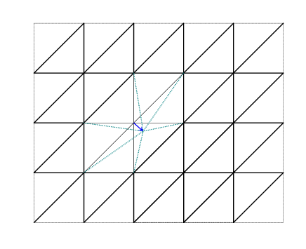
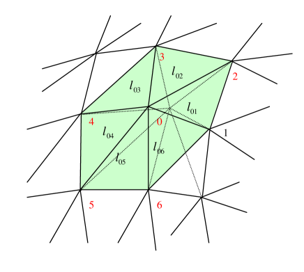
In dimensions this transformation has parameters and is an exact invariance of the action. When space is slightly curved, the invariance is in general only an approximate one, even though for piecewise linear spaces piecewise diffeomorphisms can still be defined as the set of local motions of points that leave the local contribution to the action, the measure and the lattice analogues of the continuum curvature invariants unchanged (Hamber and Williams, 1998). Note that in general the gauge deformations of the edges are still constrained by the triangle inequalities. The general situation is illustrated in Figs. 16, 17 and 18. In the limit when the number of edges becomes very large, the full continuum diffeomorphism group should be recovered.
In general the structure of lattice local gauge transformations is rather complicated and will not be given here; it can be found in the above quoted reference. These are defined as transformations acting locally on a given set of edges which leave the local lattice curvature invariant. The simplest context in which this local invariance can be exhibited explicitly is the lattice weak field expansion, which will be discussed later in Sec. III.2.1. The local gauge invariance corresponding to continuum diffeomorphism is given there in Eq. (LABEL:eq:eigenmodes). From the transformation properties of the edge lenghts it is clear that their transformation properties are related to those of the local metric, as already suggested for example by the identification of Eqs. (331) and (396).
III.1.5 Lattice Bianchi Identities
Consider therefore a closed path encircling a hinge and passing through each of the simplices that meet at that hinge. In particular one may take to be the boundary of the polyhedral dual (or Voronoi) area surrounding the hinge. We recall that the Voronoi polyhedron dual to a vertex is the set of all points on the lattice which are closer to than any other vertex; the corresponding new vertices then represent the sites on the dual lattice. A unique closed parallel transport path can then be assigned to each hinge, by suitably connecting sites in the dual lattice.
With each neighboring pair of simplices one associates a Lorentz transformation , which describes how a given vector transforms between the local coordinate systems in these two simplices As discussed previously, the above transformation is directly related to the continuum path-ordered () exponential of the integral of the local affine connection via
| (384) |
The connection here has support only on the common interface between the two simplices.
Just as in the continuum, where the affine connection and therefore the infinitesimal rotation matrix is determined by the metric and its first derivatives, on the lattice one expects that the elementary rotation matrix between simplices is fixed by the difference between the ’s of Eq. (331) within neighboring simplices.
For a vector transported once around a Voronoi loop, i.e. a loop formed by Voronoi edges surrounding a chosen hinge, the change in the vector is given by
| (385) |
where is now the total rotation matrix associated with the given hinge, given by
| (386) |
It is these lattice parallel transporters around closed elementary loops that satisfy the lattice analogues of the Bianchi identities. These are derived by considering paths which encircle more than one hinge and yet are topologically trivial, in the sense that they can be shrunk to a point without entangling any hinge (Regge, 1961).
Thus, for example, the ordered product of rotation matrices associated with the triangles meeting on a given edge has to give one, since a single path can be constructed which sequentially encircles all the triangles and is topologically trivial
| (387) |
Other identities might be derived by considering paths that encircle several hinges meeting on one point. Regge has shown that the above lattice relations correspond precisely to the continuum Bianchi identities. One can therefore explicitly construct exact lattice analogues of the continuum uncontracted, partially contracted, and fully contracted Bianchi identities (Hamber and Kagel, 2004). The lattice Bianchi identities are illustrated in Figs. 19 for the three-dimensional case, and 20 for the four-dimensional case.
The resulting lattice equations are quite similar in structure to the Bianchi identities in lattice gauge theories, where one considers identities arising from the multiplication of group elements associated with the square faces of a single cube part of a hypercubic lattice (Wilson, 1973). The motivation there was the possible replacement of the integration over the group elements by an integration over the “plaquette variables” associated with an elementary square (thereby involving the ordered product of four group elements), provided the Bianchi identity constraint is included as well in the lattice path integral.
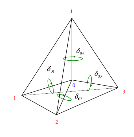
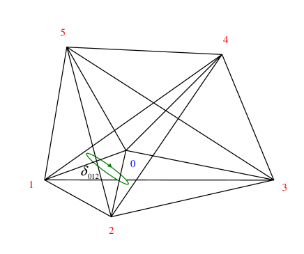
III.1.6 Gravitational Wilson Loop
We have seen that with each neighboring pair of simplices one can associate a Lorentz transformation , which describes how a given vector transforms between the local coordinate systems in these two simplices, and that the above transformation is directly related to the continuum path-ordered () exponential of the integral of the local affine connection via
| (388) |
with the connection having support only on the common interface between the two simplices. Also, for a closed elementary path encircling a hinge and passing through each of the simplices that meet at that hinge one has for the total rotation matrix associated with the given hinge
| (389) |
Equivalently, this last expression can be re-written in terms of a surface integral of the Riemann tensor, projected along the surface area element bivector associated with the loop,
| (390) |
More generally one might want to consider a near-planar, but non-infinitesimal, closed loop , as shown in Fig. 21. Along this closed loop the overall rotation matrix will still be given by
| (391) |
In analogy with the infinitesimal loop case, one would like to state that for the overall rotation matrix one has
| (392) |
where is now an area bivector perpendicular to the loop - which will work only if the loop is close to planar so that can be taken to be approximately constant along the path .

If that is true, then one can define, again in analogy with the infinitesimal loop case, an appropriate coordinate scalar by contracting the above rotation matrix with the bivector of Eq. (336), namely
| (393) |
where the loop bivector, in four dimensions, is now intended as being representative of the overall geometric features of the loop. For example, it can be taken as an average of the hinge bivector along the loop.
In the quantum theory one is of course interested in the average of the above loop operator , as in Eq. (325). The previous construction is indeed quite analogous to the Wilson loop definition in ordinary lattice gauge theories (Wilson, 1973), where it is defined via the trace of path ordered products of color rotation matrices. In gravity though the Wilson loop does not give any information about the static potential (Modanese, 1993; Hamber, 1993). It seems that the Wilson loop in gravity provides instead some insight into the large-scale curvature of the manifold, just as the infinitesimal loop contribution entering the lattice action of Eqs. (366) and (367) provides, through its averages, insight into the very short distance, local curvature. Of course for any continuum manifold one can define locally the parallel transport of a vector around a near-planar loop . Indeed parallel transporting a vector around a closed loop represents a suitable operational way of detecting curvature locally. If the curvature of the manifold is small, one can treat the larger loop the same way as the small one; then the expression of Eq. (392) for the rotation matrix associated with a near-planar loop can be re-written in terms of a surface integral of the large-scale Riemann tensor, projected along the surface area element bivector associated with the loop,
| (394) |
Thus a direct calculation of the Wilson loop provides a way of determining the effective curvature at large distance scales, even in the case where short distance fluctuations in the metric may be significant. Conversely, the rotation matrix appearing in the elementary Wilson loop of Eqs. (357) and (360) only provides information about the parallel transport of vectors around infinitesimal loops, with size comparable to the ultraviolet cutoff.
One would expect that for a geometry fluctuating strongly at short distances (corresponding therefore to the small limit) the infinitesimal parallel transport matrices should be distributed close to randomly, with a measure close to the uniform Haar measure, and with little correlation between neighboring hinges. In such instance one would have for the local quantum averages of the infinitesimal lattice parallel transports , but , which would require, for a non-vanishing lowest order contribution to the Wilson loop, that the loop at least be tiled by elementary action contributions from Eqs. (366) or (367), thus forming a minimal surface spanning the loop. Then, in close analogy to the Yang-Mills case of Eq. (326) (see for example Peskin and Schroeder, 1995), the leading contribution to the gravitational Wilson loop would be expected to follow an area law,
| (395) |
where is the minimal physical area spanned by the near-planar loop , and the gravitational correlation length at small . Thus for a close-to-circular loop of perimeter one would use .
The rapid decay of the gravitational Wilson loop as a function of the area is seen here simply as a general and direct consequence of the disorder in the fluctuations of the parallel transport matrices at strong coupling. It should then be clear from the above discussion that the gravitational Wilson loop provides in a sense a measure of the magnitude of the large-scale, averaged curvature, where the latter is most suitably defined by the process of parallel-transporting test vectors around very large loops, and is therefore, from the above expression, computed to be of the order , at least in the small limit. A direct calculation of the Wilson loop should therefore Provide, among other things, a direct insight into whether the manifold is de Sitter or anti-de Sitter at large distances. More details on the lattice construction of the gravitational Wilson loop, the various issues that arise in its precise definition, and a sample calculation in the strong coupling limit of lattice gravity, can be found in (Hamber and Williams, 2007).
Finally we note that the definition of the gravitational Wilson loop is based on a surface with a given boundary , in the simplest case the minimal surface spanning the loop. It is possible though to consider other surfaces built out of elementary parallel transport loops. An example of such a generic closed surface tiled with elementary parallel transport polygons (here chosen for illustrative purposes to be triangles) will be given later in Fig. 29.
Later similar surfaces will arise naturally in the context of the strong coupling (small ) expansion for gravity, as well as in the high dimension (large ) expansion.
III.1.7 Lattice Regularized Path Integral
As the edge lengths play the role of the continuum metric , one would expect the discrete measure to involve an integration over the squared edge lengths (Hamber, 1984; Hartle, 1984; Hamber and Williams, 1999). Indeed the induced metric at a simplex is related to the squared edge lengths within that simplex, via the expression for the invariant line element . After choosing coordinates along the edges emanating from a vertex, the relation between metric perturbations and squared edge length variations for a given simplex based at 0 in dimensions is
| (396) |
For one -dimensional simplex labeled by the integration over the metric is thus equivalent to an integration over the edge lengths, and one has the identity
| (397) |
There are edges for each simplex, just as there are independent components for the metric tensor in dimensions (Cheeger, Müller and Schrader, 1981). Here one is ignoring temporarily the triangle inequality constraints, which will further require all sub-determinants of to be positive, including the obvious restriction .
Let us discuss here briefly the simplicial inequalities that need to be imposed on the edge lengths (Wheeler 1964). These are conditions on the edge lengths such that the sites can then be considered the vertices of a -simplex embedded in flat -dimensional Euclidean space. In one dimension, , one requires trivially for all edge lengths
| (398) |
In two dimensions, , the conditions on the edge lengths are again as in one dimensions, as well as
| (399) |
which is equivalent, by virtue of Heron’s formula for the area of a triangle where is the semi-perimeter , to the requirement that the area of the triangle be positive. In turn Eq. (399) implies that the triangle inequalities must be satisfied for all three edges,
| (400) |
In three dimensions, , the conditions on the edge lengths are again such that one recovers a physical tetrahedron. One therefore requires for the individual edge lengths the condition of Eq. (398), the reality and positivity of all four triangle areas as in Eq. (399), as well as the requirement that the volume of the tetrahedron be real and positive,
| (401) |
The generalization to higher dimensions is such that one requires all triangle inequalities and their higher dimensional analogues to be satisfied,
| (402) |
with for every possible choice of sub-simplex (and therefore sub-determinant) within the original simplex .
The extension of the measure to many simplices glued together at their common faces is then immediate. For this purpose one first needs to identify edges and which are shared between simplices and ,
| (403) |
After summing over all simplices one derives, up to an irrelevant numerical constant, the unique functional measure for simplicial geometries
| (404) |
Here is a (step) function of the edge lengths, with the property that it is equal to one whenever the triangle inequalities and their higher dimensional analogues are satisfied, and zero otherwise. The quantity has been introduced as a cutoff at small edge lengths. If the measure is non-singular for small edges, one can safely take the limit . In four dimensions the lattice analog of the DeWitt measure () takes on a particularly simple form, namely
| (405) |
Lattice measures over the space of squared edge lengths have been used extensively in numerical simulations of simplicial quantum gravity (Hamber and Williams, 1984; Hamber, 1984; Berg 1985). The derivation of the above lattice measure closely parallels the analogous procedure in the continuum.
There is no obstacle in defining a discrete analog of the supermetric, as a way of introducing an invariant notion of distance between simplicial manifolds, as proposed in (Cheeger, Müller and Schrader, 1984). It leads to an alternative way of deriving the lattice measure in Eq. (405), by considering the discretized distance between induced metrics
| (406) |
with the inverse of the lattice DeWitt supermetric now given by the expression
| (407) |
and with again . This procedure defines a metric on the tangent space of positive real symmetric matrices . After computing the determinant of , the resulting functional measure is
| (408) |
with the determinant of the super-metric given by the local expression
| (409) |
Using Eq. (397), and up to irrelevant constants, one obtains again the standard lattice measure of Eq. (404). Of course the same procedure can be followed for the Misner-like measure, leading to a similar result for the lattice measure, but with a different power .
One might be tempted to try to find alternative lattice measures by looking directly at the discrete form for the supermetric, written as a quadratic form in the squared edge lengths (instead of the metric components), and then evaluating the resulting determinant. The main idea, inspired by work described in a paper (Lund and Regge, 1974) on the formulation of simplicial gravity, is as follows. First one considers a lattice analog of the DeWitt supermetric by writing
| (410) |
with now defined on the space of squared edge lengths (Hartle, Miller and Williams, 1997). The next step is to find an appropriate form for expressed in terms of known geometric objects. One simple way of constructing the explicit form for , in any dimension, is to first focus on one simplex, and write the squared volume of a given simplex in terms of the induced metric components within the same simplex ,
| (411) |
One computes to linear order
| (412) |
and to quadratic order
| (413) |
The right hand side of this equation contains precisely the expression appearing in the continuum supermetric of Eq. (162), for the specific choice of the parameter . One is led therefore to the identification
| (414) |
and therefore for the norm
| (415) |
One could be tempted at this point to write down a lattice measure, in parallel with Eq. (164), and write
| (416) |
with
| (417) |
where one has allowed for a parameter , possibly different from zero, interpolating between apparently equally acceptable measures. The reasoning here is that, as in the continuum, different edge length measures, here parametrized by ’, are obtained, depending on whether the local volume factor is included in the supermetric or not.
One rather undesirable, and puzzling, feature of the lattice measure of Eq. (416) is that in general it is non-local, in spite of the fact that the original continuum measure of Eq. (166) is completely local (although it is clear that for some special choices of and , one does recover a local measure; thus in two dimensions and for one obtains again the simple result ). Unfortunately irrespective of the value chosen for , one can show (Hamber and Williams, 1999) that the measure of Eq. (416) disagrees with the continuum measure of Eq. (166) already to lowest order in the weak field expansion, and does not therefore describe an acceptable lattice measure.
The lattice action for pure four-dimensional Euclidean gravity contains a cosmological constant and Regge scalar curvature term
| (418) |
with , as well as possibly higher derivative terms. It only couples edges which belong either to the same simplex or to a set of neighboring simplices, and can therefore be considered as local, just like the continuum action, and leads to the regularized lattice functional integral
| (419) |
where, as customary, the lattice ultraviolet cutoff is set equal to one (i.e. all length scales are measured in units of the lattice cutoff).
The lattice partition function should then be compared to the continuum Euclidean Feynman path integral of Eq. (182),
| (420) |
Occasionally it can be convenient to include the -term in the measure. For this purpose one defines
| (421) |
It should be clear that this last expression represents a fairly non-trivial quantity, both in view of the relative complexity of the expression for the volume of a simplex, Eq. (333), and because of the generalized triangle inequality constraints already implicit in . But, like the continuum functional measure, it is certainly local, to the extent that each edge length appears only in the expression for the volume of those simplices which explicitly contain it. Furthermore, sets the overall scale and can therefore be set equal to one without any loss of generality.
III.1.8 An Elementary Example
In the very simple case of one dimension () one can work out explicitly a number of details, and see how potential problems with the functional measure arise, and how they are resolved.
In one dimension one discretizes the line by introducing points, with lengths associated with the edges, and periodic boundary conditions, . Here is the distance between points and . The only surviving invariant term in one dimension is then the overall length of a curve,
| (422) |
which corresponds to
| (423) |
(with ) in the continuum. Here is the “einbein”, and satisfies the obvious constraint . In this context the discrete action is unique, preserving the geometric properties of the continuum definition. From the expression for the invariant line element, , one associates with (and therefore with ). One can further take the view that distances can only be assigned between vertices which appear on some lattice in the ensemble, although this is not strictly necessary, as distances can also be defined for locations that do not coincide with any specific vertex.
The gravitational measure then contains an integration over the elementary lattice degrees of freedom, the lattice edge lengths. For the edges one writes the lattice integration measure as
| (424) |
where is a parameter interpolating between different local measures. The positivity of the edge lengths is all that remains of the triangle inequality constraints in one dimension. The factor plays a role analogous to the which appears for continuum measures in the Euclidean functional integral.
The functional measure does not have compact support, and the cosmological term (with a coefficient ) is therefore necessary to obtain convergence of the functional integral, as can be seen for example from the expression for the average edge length,
| (425) |
with
| (426) |
Similarly one finds for the fluctuation in the total length , which requires . Different choices for then correspond to trivial rescalings of the average lattice spacing, .
In the continuum, the action of Eq. (423) is invariant under continuous reparametrizations
| (427) |
| (428) |
or equivalently
| (429) |
and we have set . A gauge can then be chosen by imposing , which can be achieved by the choice of coordinates .
The discrete analog of the transformation rule is
| (430) |
where the ’s represent continuous gauge transformations defined on the lattice vertices. In order for the edge lengths to remain positive, one needs to require , which is certainly satisfied for sufficiently small ’s. The above continuous symmetry is an exact invariance of the lattice action of Eq. (422), since
| (431) |
and we have used . Moreover, it is the only local symmetry of the action of Eq. (422).
The infinitesimal local invariance property defined in Eq. (430) formally selects a unique measure over the edge lengths, corresponding to ( in Eq. (424)), as long as we ignore the effects of the lower limit of integration. On the other hand for sufficiently large lattice diffeomorphisms, the lower limit of integration comes into play (since we require always) and the measure is no longer invariant. Thus a measure would not be acceptable on physical grounds; it would violate the constraint or .
The same functional measure can be obtained from the following physical consideration. Define the gauge invariant distance between two configurations of edge lengths and by
| (432) |
with . Since is independent of and , the ensuing measure is again simply proportional to . Note that the above metric over edge length deformations is non-local.
In the continuum, the functional measure is usually determined by considering the following (local) norm in function space,
| (433) |
and diffeomorphism invariance would seem to require . The volume element in function space is then an ultraviolet regulated version of , which is the Misner measure in one dimension. Its naive discrete counterpart would be , which is not invariant under the transformation of Eq. (430) (it is invariant under , which is not an invariance of the action).
The point of the discussion of the one-dimensional case is to bring to the surface the several non-trivial issues that arise when defining a properly regulated version of the continuum Feynman functional measure , and how they can be systematically resolved.
III.1.9 Lattice Higher Derivative Terms
So far only the gravitational Einstein-Hilbert contribution to the lattice action and the cosmological constant term have been considered. There are several motivations for extending the discussion to lattice higher derivative terms, which would include the fact that these terms a) might appear in the original microscopic action, or might have to be included to cure the classical unboundedness problem of the Euclidean Einstein-Hilbert action, b) that they are in any case generated by radiative corrections, and c) that on a more formal level they may shed new light on the relationship between the lattice and continuum expressions for curvature terms as well as quantities such as the Riemann tensor on a hinge, Eq. (364).
For these reasons we will discuss here a generalization of the Regge gravity equivalent of the Einstein action to curvature squared terms. When considering contributions quadratic in the curvature there are overall six possibilities, listed in Eq. (93). Among the two topological invariants, the Euler characteristic for a simplicial decomposition may be obtained from a particular case of the general formula for the analog of the Lipschitz-Killing curvatures of smooth Riemannian manifolds for piecewise flat spaces. The formula of (Cheeger, Müller and Schrader, 1984) reduces in four dimensions to
| (434) |
where denotes an i-dimensional simplex and denotes the (internal) dihedral angle at an i-dimensional face of a j-dimensional simplex. Thus, for example, is the angle at the vertex of a triangle and is the dihedral angle at a triangle in a 4-simplex (The normalization of the angles is such that the volume of a sphere in any dimension is one; thus planar angles are divided by , 3-dimensional solid angles by and so on).
Of course, as noted before, there is a much simpler formula for the Euler characteristic of a simplicial complex
| (435) |
where is the number of simplices of dimension . However, it may turn out to be useful in quantum gravity calculations to have a formula for in terms of the angles, and hence of the edge lengths, of the simplicial decomposition. These expression are interesting and useful, but do not shed much light on how the other curvature squared terms should be constructed.
In a piecewise linear space curvature is detected by going around elementary loops which are dual to a ()-dimensional subspace. The area of the loop itself is not well defined, since any loop inside the -dimensional simplices bordering the hinge will give the same result for the deficit angle. On the other hand the hinge has a content (the length of the edge in and the area of the triangle in ), and there is a natural volume associated with each hinge, defined by dividing the volume of each simplex touching the hinge into a contribution belonging to that hinge, and other contributions belonging to the other hinges on that simplex (Hamber and Williams, 1984). The contribution belonging to that simplex will be called dihedral volume . The volume associated with the hinge is then naturally the sum of the dihedral volumes belonging to each simplex
| (436) |
The dihedral volume associated with each hinge in a simplex can be defined using dual volumes, a barycentric subdivision, or some other natural way of dividing the volume of a -simplex into parts. If the theory has some reasonable continuum limit, then the final results should not depend on the detailed choice of volume type.

As mentioned previously, there is a well-established procedure for constructing a dual lattice for any given lattice. This involves constructing polyhedral cells, known in the literature as Voronoi polyhedra, around each vertex, in such a way that the cell around each particular vertex contains all points which are nearer to that vertex than to any other vertex. Thus the cell is made up from ()-dimensional subspaces which are the perpendicular bisectors of the edges in the original lattice, ()-dimensional subspaces which are orthogonal to the 2-dimensional subspaces of the original lattice, and so on. General formulas for dual volumes are given in (Hamber and Williams, 1986). In the case of the barycentric subdivision, the dihedral volume is just times the volume of the simplex. This leads one to conclude that there is a natural area associated with each hinge
| (437) |
obtained by dividing the volume per hinge (which is -dimensional) by the volume of the hinge (which is ()-dimensional).
The next step is to find terms equivalent to the continuum expression of Eq. (93), and the remainder of this section will be devoted to this problem. It may be objected that since in Regge calculus where the curvature is restricted to the hinges which are subspaces of dimension 2 less than that of the space considered, then the curvature tensor involves -functions with support on the hinges, and so higher powers of the curvature tensor are not defined. But this argument clearly does not apply to the Euler characteristic and the Hirzebruch signature of Eq. Eq. (93), which are both integrals of 4-forms. However it is a common procedure in lattice field theory to take powers of fields defined at the same point, and there is no reason why one should not consider similar terms in lattice gravity. Of course one would like the expressions to correspond to the continuum ones as the edge lengths of the simplicial lattice become smaller and smaller.
Since the curvature is restricted to the hinges, it is natural that expressions for curvature integrals should involve sums over hinges as in Eq. (366). The curvature tensor, which involves second derivatives of the metric, is of dimension . Therefore is of dimension . Thus if one postulates that an -type term will involve the square of , which is of dimension , then one will need to divide by some -dimensional volume to obtain the correct dimension for the extra term in the action. Now any hinge is surrounded by a number of -dimensional simplices, so the procedure of dividing by a -dimensional volume seems ambiguous. The crucial step is to realize that there is a unique -dimensional volume associated with each hinge, as described above.
If one regards the invariant volume element as being represented by of Eq. (436) when one performs the sum over hinges as in Eq. (366), then this means that one may regard the scalar curvature contribution as being represented at each hinge by
| (438) |
It is then straightforward to see that a candidate curvature squared term is
| (439) |
where was defined in Eq. 437). Since the expression in Eq. (439) vanishes if and only if all deficit angles are zero, it is naturally identified with the continuum Riemann squared term,
| (440) |
The above construction then leaves open the question of how to construct the remaining curvature squared terms in four dimensions. If one takes the form given previously in Eq. (364) for the Riemann tensor on a hinge and contracts one obtains
| (441) |
which agrees with the form used in the Regge action for . But one also finds readily that with this choice the higher derivative terms are all proportional to each other (Hamber and Williams, 1986),
| (442) |
Furthermore if one uses the above expression for the Riemann tensor to evaluate the contribution to the Euler characteristic on each hinge one obtains zero, and becomes clear that at least in this case one needs cross terms involving contributions from different hinges.
The next step is therefore to embark on a slightly more sophisticated approach, and construct the full Riemann tensor by considering more than one hinge. Define the Riemann tensor for a simplex as a weighted sum of hinge contributions
| (443) |
where the are dimensionless weights, to be determined later. After squaring one obtains
| (444) |
The question of the weights introduced in Eq. (443) will now be addressed. Consider the expression for the scalar curvature of a simplex defined as
| (445) |
It is clear from the formulae given above for the lattice curvature invariants (constructed in a simplex by summing over hinge contributions) that there is again a natural volume associated with them : the sum of the volumes of the hinges in the simplex
| (446) |
where is the volume around the hinge, as defined in Eq. (436). Summing the scalar curvature over all simplices, one should recover Regge’s expression
| (447) |
which implies
| (448) |
where is the number of simplices meeting on that hinge. Therefore the correct choice for the weights is
| (449) |
Thus the weighting factors that reproduce Regge’s formula for the Einstein action are just the volume fractions occupied by the various hinges in a simplex, which is not surprising (of course the above formulae are not quite unique, since one might have done the above construction of higher derivative terms by considering a point instead of a four-simplex ).
In particular the following form for the Weyl tensor squared was given in (Hamber and Williams, 1986)
| (450) |
which introduces a short range coupling between deficit angles. The numerical factor is equal to if the two hinges have one edge in common and if they do not. Note that this particular interaction term has the property that it requires neighboring deficit angles to have similar values, but it does not require them to be small, which is a key property one would expect from the Weyl curvature squared term.
In conclusion the formulas given above allow one to construct the remaining curvature squared terms in four dimensions, and in particular to write, for example, the lattice analog of the continuum curvature squared action of Eq. (103)
| (451) | |||||
To compare with the form of Eq. (103) use has been made of and , up to additive constant contributions. A special case corresponds to , which gives a pure contribution. The latter vanishes if and only if the curvature is locally zero, which is not true of any of the other curvature squared terms.
III.1.10 Scalar Matter Fields
In the previous section we have discussed the construction and the invariance properties of a lattice action for pure gravity. Next a scalar field can be introduced as the simplest type of dynamical matter that can be coupled invariantly to gravity. In the continuum the scalar action for a single component field is usually written as
| (452) |
where the dots denote scalar self-interaction terms. Thus for example a scalar field potential could be added containing quartic field terms, whose effects could be of interest in the context of cosmological models where spontaneously broken symmetries play an important role. The dimensionless coupling is arbitrary; two special cases are the minimal () and the conformal () coupling case. In the following we shall mostly consider the case . Also, it will be straightforward to extend later the treatment to the case of an -component scalar field with .
One way to proceed is to introduce a lattice scalar defined at the vertices of the simplices. The corresponding lattice action can then be obtained through a procedure by which the original continuum metric is replaced by the induced lattice metric, with the latter written in terms of squared edge lengths as in Eq. (331). For illustrative purposes only the two-dimensional case will be worked out explicitly here (Christ, Friedberg and Lee, 1982; Itzykson, 1983; Bander and Itzykson, 1983; Jevicki and Ninomiya, 1984). The generalization to higher dimensions is straightforward, and in the end the final answer for the lattice scalar action is almost identical to the two dimensional form. Furthermore in two dimensions it leads to a natural dicretization of the bosonic string action (Polyakov, 1989).
In two dimensions the simplicial lattice is built out of triangles. For a given triangle it will be convenient to use the notation of Fig. 23, which will display more readily the symmetries of the resulting scalar lattice action. Here coordinates will be picked in each triangle along the (1,2) and (1,3) directions.
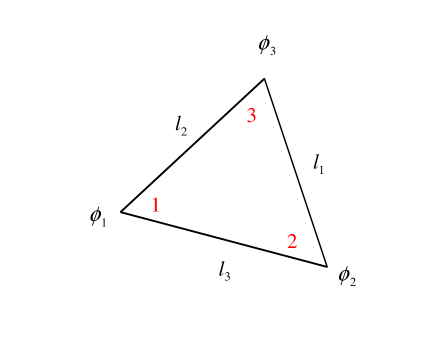
To construct a lattice action for the scalar field, one performs in two dimensions the replacement
| (453) |
with the following definitions
| (454) |
| (455) |
| (456) |
The scalar field derivatives get replaced as usual by finite differences
| (457) |
where the index labels the possible directions in which one can move away from a vertex within a given triangle. Then
| (458) |
Then the discrete scalar field action takes the form
| (459) |
where the sum is over all triangles on the lattice. Using the identity
| (460) |
one obtains after some re-arrangements the slightly more appealing expression for the action of a massless scalar field (Bander and Itzykson, 1984)
| (461) |
is the dual (Voronoi) area associated with the edge , and the symbol denotes a sum over nearest neighbor lattice vertices. It is immediate to generalize the action of Eq. (461) to higher dimensions, with the two-dimensional Voronoi volumes replaced by their higher dimensional analogues, leading to
| (462) |
Here is the dual (Voronoi) volume associated with the edge , and the sum is over all links on the lattice.
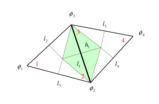
In two dimensions, in terms of the edge length and the dual edge length , connecting neighboring vertices in the dual lattice, one has (see Fig. 24). Other choices for the lattice subdivision will lead to a similar formula for the lattice action, with the Voronoi dual volumes replaced by their appropriate counterparts for the new lattice. Explicitly, for an edge of length the dihedral dual volume contribution is given by
| (463) |
with is the length of the edge dual to .
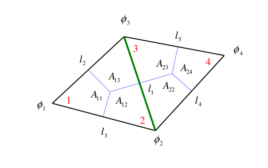
On the other hand the barycentric dihedral area for the same edge would be simply
| (464) |
It is well known that one of the disadvantages of the Voronoi construction is the lack of positivity of the dual volumes, as pointed out in (Hamber and Williams, 1984). Thus some of the weights appearing in Eq. (461) can be negative for such an action. For the barycentric subdivision this problem does not arise, as the areas are always positive due to the enforcement of the triangle inequalities. Thus from a practical point of view the barycentric volume subdivision is the simplest to deal with.
The scalar action of Eq. (462) has a very natural form: it involves the squared difference of fields at neighboring points divided by their invariant distances , weighted by the appropriate space-time volume element associated with the lattice link . This suggests that one could just as well define the scalar fields on the vertices of the dual lattice, and write
| (465) |
with the length of the edge connecting the dual lattice vertices and , and consequently the spacetime volume fraction associated with the dual lattice edge . One would expect both forms to be equivalent in the continuum limit.
Continuing on with the two-dimensional case, mass and curvature terms such as the ones appearing in Eq. (452) can be added to the action, so that the total scalar lattice action contribution becomes
| (466) |
The term containing the discrete analog of the scalar curvature involves the quantity
| (467) |
In the above expression for the scalar action, is the area associated with the edge , while is associated with the site . Again there is more than one way to define the volume element , (Hamber and Williams, 1986), but under reasonable assumptions, such as positivity, one expects to get equivalent results in the lattice continuum limit, if it exists.
In higher dimensions one would use
| (468) |
where the term containing the discrete analog of the scalar curvature involves
| (469) |
In the expression for the scalar action, is the (dual) volume associated with the edge , while is the (dual) volume associated with the site .
The lattice scalar action contains a mass parameter , which has to be tuned to zero in lattice units to achieve the lattice continuum limit for scalar correlations. The agreement between different lattice actions in the smooth limit can be shown explicitly in the lattice weak field expansion. But in general, as is already the case for the purely gravitational action, the correspondence between lattice and continuum operators is true classically only up to higher derivative corrections. But such higher derivative corrections in the scalar field action are expected to be irrelevant when looking at the large distance limit, and they will not be considered here any further.
As an extreme case one could even consider a situation in which the matter action by itself is the only action contribution, without any additional term for the gravitational field, but still with a non-trivial gravitational measure; integration over the scalar field would then give rise to an effective non-local gravitational action.
Finally let us take notice here of the fact that if an -component scalar field is coupled to gravity, the power appearing in the gravitational functional measure has to be modified to include an additional factor of . The additional measure factor insures that the integral
| (470) |
evaluates to a constant. Thus for large mass the scalar field completely decouples, leaving only the dynamics of the pure gravitational field.
The quadratic scalar field action of Eq. (462) can be written in terms of a matrix
| (471) |
The matrix can then be regarded as a lattice version of the continuum scalar Laplacian,
| (472) |
for a given background metric. This then allows one to define the massless lattice scalar propagator as the inverse of the above matrix, . The continuum scalar propagator for a finite scalar mass and in a given background geometry, evaluated for large separations ,
| (473) | |||||
involves the geodesic distance between points and ,
| (474) |
Analogously, one can define the discrete massive lattice scalar propagator
| (475) | |||||
where is the lattice geodesic distance between vertex and vertex . The inverse can be computed, for example, via the recursive expansion (valid for to avoid the zero eigenvalue of the Laplacian)
| (476) |
The large distance behavior of the Euclidean (flat space) massive free field propagator in dimensions is known in the statistical mechanics literature as the Ornstein-Zernike result.
As a consequence, the lattice propagator can be used to estimate the lattice geodesic distance between any two lattice points and in a fixed background lattice geometry (provided again that their mutual separation is such that ).
| (477) |
III.1.11 Invariance Properties of the Scalar Action
In the very simple case of one dimension () one can work out the details to any degree of accuracy, and see how potential problems arise and how they are resolved. Introduce a scalar field defined on the sites, with action
| (478) |
with . It is natural in one dimension to take for the “volume per edge” , and for the “volume per site” . Here plays the role of a mass for the scalar field, . In addition one needs a term
| (479) |
which is necessary in order to make the integration convergent at large . Varying the action with respect to gives
| (480) |
This is the discrete analog of the equation . The spectrum of the Laplacian of Eq. (480) corresponds to . Variation with respect to gives instead
| (481) |
For it suggests the well-known interpretation of the fields as coordinates in embedding space. In the following we shall only consider the case , corresponding to a massless scalar field.
It is instructive to look at the invariance properties of the scalar field action under the continuous lattice diffeomorphisms defined in Eq. (430). Physically, these local gauge transformations, which act on the vertices, correspond to re-assignments of edge lengths which leave the distance between two fixed points unchanged. In the simplest case, only two neighboring edge lengths are changed, leaving the total distance between the end points unchanged. On physical grounds one would like to maintain such an invariance also in the case of coupling to matter, just as is done in the continuum.
The scalar nature of the field requires that in the continuum under a change of coordinates ,
| (482) |
where and refer to the same physical point in the two coordinate systems. On the lattice, as discussed previously, diffeomorphisms move the points around, and at the same vertex labeled by we expect
| (483) |
One can determine the exact form of the change needed in by requiring that the local variation of the scalar field action be zero. Solving the resulting quadratic equation for one obtains a rather unwieldy expression, given to lowest order by
| (484) | |||||
and which is indeed of the expected form (as well as symmetric in the vertices and ). For fields which are reasonably smooth, this correction is suppressed if . On the other hand it should be clear that the measure is no longer manifestly invariant, due to the rather involved transformation property of the scalar field.
The full functional integral for sites then reads
| (485) |
In the absence of the scalar field one just has the of Eq. (426). The trivial translational mode in can be eliminated for example by setting .
It is possible to further constrain the measure over the edge lengths by examining some local averages. Under a rescaling of the edge lengths one can derive the following identity for
| (486) |
where we have replaced the coefficient of the scalar kinetic term by . It follows then that
| (487) |
and
| (488) |
Without loss of generality we can fix the average edge length to be equal to one, , which then requires . In order for the model to be meaningful, the measure parameter is constrained by , i.e. the measure over the edges cannot be too singular.
III.1.12 Lattice Fermions, Tetrads and Spin Rotations
On a simplicial manifold spinor fields and are most naturally placed at the center of each d-simplex . In the following we will restrict our discussion for simplicity to the four-dimensional case, and largely follow the original discussion given by (Fröhlich, 1981) and (Drummond 1986). As in the continuum (see for example Veltman, 1974), the construction of a suitable lattice action requires the introduction of the Lorentz group and its associated tetrad fields within each simplex labeled by .
Within each simplex one can choose a representation of the Dirac gamma matrices, denoted here by , such that in the local coordinate basis
| (489) |
These in turn are related to the ordinary Dirac gamma matrices , which obey
| (490) |
by
| (491) |
so that within each simplex the tetrads satisfy the usual relation
| (492) |
In general the tetrads are not fixed uniquely within a simplex, being invariant under the local Lorentz transformations discussed earlier in Sec. III.1.2.
In the continuum the action for a massless spinor field is given by
| (493) |
where is the spinorial covariant derivative containing the spin connection . It will be convenient to first consider only two neighboring simplices and , covered by a common coordinate system . When the two tetrads in and are made to coincide, one can then use a common set of gamma matrices within both simplices. Then in the absence of torsion the covariant derivative in Eq. (493) reduces to just an ordinary derivative. The fermion field within the two simplices can then be suitably interpolated, by writing for example
| (494) |
where is the common normal to the face shared by the simplices and , and chosen to point into . Inserting the expression for from Eq. (494) into Eq. (493) and applying the divergence theorem (or equivalently using the fact that the derivative of a step function only has support at the origin) one obtains
| (495) |
where represents the volume of the -dimensional common interface , a tetrahedron in four dimensions. But the contributions from the diagonal terms containing and vanish when summed over the faces of an -simplex, by virtue of the useful identity
| (496) |
where are the volumes of the faces of a given simplex, and the inward pointing unit normals to those faces.
So far the above partial expression for the lattice spinor action was obtained by assuming that the tetrads and in the two simplices coincide. If they do not, then they will be related by a matrix such that
| (497) |
and whose spinorial representation was given previously for example in Eq. (352). Such a matrix is now needed to additionally parallel transport the spinor from a simplex to the neighboring simplex .
The invariant lattice action for a massless spinor takes therefore the form
| (498) |
where the sum extends over all interfaces connecting one simplex to a neighboring simplex . As shown in (Drummond 1986) it can be further extended to include a dynamical torsion field.
The above spinorial action can be considered analogous to the lattice Fermion action proposed originally in (Wilson 1973) for non-Abelian gauge theories. It is possible that it still suffers from the Fermion doubling problem, although the situation is less clear for a dynamical lattice (Nielsen and Ninomiya, 1981; Christ and Lee, 1982).
III.1.13 Alternate Discrete Formulations
The simplicial lattice formulation offers a natural way of representing gravitational degrees in a discrete framework by employing inherently geometric concepts such as areas, volumes and angles. It is possible though to formulate quantum gravity on a flat hypercubic lattice, in analogy to Wilson’s discrete formulation for gauge theories, by putting the connection center stage. In this new set of theories the natural variables are then lattice versions of the spin connection and the vierbein. Also, because the spin connection variables appear from the very beginning, it is much easier to incorporate fermions later. Some lattice models have been based on the pure Einstein theory (Smolin, 1979; Das, Kaku and Townsend, 1979; Mannion and Taylor, 1981; Caracciolo and Pelissetto, 1987), while others attempt to incorporate higher derivative terms (Tomboulis 1984; Kondo 1984).
Difficult arise when attempting to put quantum gravity on a flat hypercubic lattice a la Wilson, since it is not entirely clear what the gravity analog of the Yang-Mills connection is. In continuum formulations invariant under the Poincaré or de Sitter group the action is invariant under a local extension of the Lorentz transformations, but not under local translations (Kibble, 1961). Local translations are replaced by diffeomorphisms which have a different nature. One set of lattice discretizations starts from the action of (MacDowell and Mansouri, 1977; West, 1978) whose local invariance group is the de Sitter group . In the lattice formulation of (Smolin, 1979; Das, Kaku and Townsend, 1979) the lattice variables are gauge potentials and defined on lattice sites , generating local matrix transformations with the aid of the de Sitter generators and . The resulting lattice action reduces classically to the Einstein action with cosmological term in first order form in the limit of the lattice spacing ; to demonstrate the quantum equivalence one needs an additional zero torsion constraint. In the end the issue of lattice diffeomorphism invariance remains somewhat open, with the hope that such an invariance will be restored in the full quantum theory.
As an example, we will discuss here the approach of (Mannion and Taylor, 1981) which relies on a four-dimensional lattice discretization of the Einstein-Cartan theory with gauge group , and does not initially require the presence of a cosmological constant, as would be the case if one had started out with the de Sitter group . On a lattice of spacing with vertices labelled by and directions by one relates the relative orientations of nearest-neighbor local frames by
| (499) |
with , being the set of six generators of , the covering group of the Lorentz group , usually taken to be
| (500) |
with ’s the Dirac gamma matrices. The local lattice curvature is then obtained in the usual way by computing the product of four parallel transport matrices around an elementary lattice square,
| (501) |
giving in the limit of small by the Baker-Hausdorff formula the value , where is the Riemann tensor defined in terms of the spin connection
| (502) |
If one were to write for the action the usual Wilson lattice gauge form
| (503) |
then one would obtain a curvature squared action proportional to instead of the Einstein-Hilbert one. One needs therefore to introduce lattice vierbeins on the sites by defining the matrices
| (504) |
Then a suitable lattice action is given by
| (505) |
The latter is invariant under local transformations defined on the lattice vertices
| (506) |
for which the curvature transforms as
| (507) |
and the vierbein matrices as
| (508) |
Since commutes with , the expression in Eq. (505) is invariant. The metric is then obtained as usual by
| (509) |
From the expression for the lattice curvature given above if follows immediately that the lattice action in the continuum limit becomes
| (510) |
which is the Einstein action in Cartan form
| (511) |
with the parameter identified with the Planck length. One can add more terms to the action; in this theory a cosmological term can be represented by
| (512) |
Both Eqs. (505) and Eq. (512) are locally invariant. The functional integral is then given by
| (513) |
and from it one can then compute suitable quantum averages. Here is the Haar measure for ; it is less clear how to choose the integration measure over the ’s, and how it should suitably constrained, which obscure the issue of diffeomorphism invariance in this theory.
In these theories it is possible to formulate curvature squared terms as well. In general for a hypercubic lattices the formulation of -type terms in four dimensions involves constraints between the connections and the tetrads, which are a bit difficult to handle. Also there is no simple way of writing down topological invariants, which are either related to the Einstein action (in two dimensions), or are candidates for extra terms to be included in the action. A flat hypercubic lattice action has been written with higher derivative terms which appears to be reflection positive but has a very cumbersome form. These difficulties need not be present on a simplicial lattice (except that it is not known how to write an exact expression for the Hirzebruch signature in lattice terms).
There is another way of discretizing gravity, still using largely geometric concepts as is done in the Regge theory. In the dynamical triangulation approach one fixes the edge lengths to unity, and varies the incidence matrix. As a result the volume of each simplex is fixed at
| (514) |
and all dihedral angles are given by the constant value
| (515) |
so that for example in four dimensions one has . Local curvatures are then determined by how many simplices meet on a given hinge,
| (516) |
The action contribution from a single hinge is therefore from Eq. (366) with a positive integer. The local curvatures are inherently discrete, and there is no equivalent lattice notion of continuous diffeomorphisms, or for that matter of continuous local deformations corresponding for example to shear waves. The hope is that for lattices made of some large number of simplices one recovers some sort of discrete version of diffeomorphism invariance. The Euclidean dynamical triangulation approach has been reviewed recently in (Ambjørn, Carfora and Marzuoli, 1999), and we refer the reader to further references therein. A recent discussion of attempts at simulating the Lorentzian case, which leads to complex weights in the functional integral which are difficult to handle, can be found in (Loll et al, 2006).
Another lattice approach closely related to the Regge theory described in this review is based on the so-called spin foam models, which have their origin in an observation found in (Ponzano and Regge, 1968) relating the geometry of simplicial lattices to the asymptotics of Racah angular momentum addition coefficients. The original Regge-Ponzano concepts were later developed into a spin model for gravity (Hasslacher and Perry, 1981) based on quantum spin variables attached to lattice links. In these models representations of label edges. One natural underlying framework for such theories is the canonical approach to quantum gravity, wherein quantum spin variables are naturally related to spin connections. Extensions to four dimensions have been attempted, and we refer the reader to the recent review of spin foam models in (Perez, 2003).
III.2 Analytical Expansion Methods
The following sections will discuss a number of instances where the lattice theory of quantum gravity can be investigated analytically, subject to some simplifying assumptions.
The first problem is the lattice weak field expansion about a flat background. It will be shown that in this case the relevant modes are the lattice analogues of transverse-traceless deformations.
The second problem is the strong coupling (large ) expansion, where the weight factor in the path integral is expanded in powers of . The domain of validity of this expansion can be regarded as somewhat complementary to the weak field limit.
The third case to be discussed is what happens in lattice gravity in the limit of large dimensions , which formally is similar in some ways to the large- expansion discussed previously in this review. In this limit one can derive exact estimates for the phase transition point and for the scaling dimensions.
III.2.1 Lattice Weak Field Expansion and Transverse-Traceless Modes
One of the simplest possible problems that can be treated in quantum Regge calculus is the analysis of small fluctuations about a fixed flat Euclidean simplicial background (Roček and Williams, 1981). In this case one finds that the lattice graviton propagator in a De Donder-like gauge is precisely analogous to the continuum expression.
To compute an expansion of the lattice Regge action
| (517) |
to quadratic order in the lattice weak fields one needs first and second variations with respect to the edge lengths. In four dimensions the first variation of the lattice Regge action is given by
| (518) |
since Regge has shown that the term involving the variation of the deficit angle vanishes (here the variation symbol should obviously not be confused with the deficit angle). Furthermore in flat space all the deficit angles vanish, so that the second variation is given simply by
| (519) |
Next a specific lattice structure needs to be chosen as a background geometry. A natural choice is to use a flat hypercubic lattice, made rigid by introducing face diagonals, body diagonals and hyperbody diagonals, which results into a subdivision of each hypercube into (here 4!=24) simplices. This subdivision is shown in Fig. 26.

By a simple translation, the whole lattice can then be constructed from this one elemental hypercube. Consequently there will be lattice fields per point, corresponding to all the edge lengths emanating in the positive lattice directions from any one vertex. Note that the number of degrees per lattice point is slightly larger than what one would have in the continuum, where the metric has degrees of freedom per spacetime point in four dimensions (perturbatively, the physical degrees of freedom in the continuum are much less: = , for a traceless symmetric tensor, and after imposing gauge conditions). Thus in four dimensions each lattice hypercube will contain 4 body principals, 6 face diagonals, 4 body diagonals and one hyperbody diagonal. Within a given hypercube it is quite convenient to label the coordinates of the vertices using a binary notation, so that the four body principals with coordinates will be labeled by integers 1,2,4,8, and similarly for the other vertices (thus for example the vertex , corresponding to a face diagonal along the second and third Cartesian direction, will be labeled by the integer 6).
For a given lattice of fixed connectivity, the edge lengths are then allowed to fluctuate around an equilibrium value
| (520) |
In the case of the hypercubic lattice subdivided into simplices, the unperturbed edge lengths take on the values , depending on edge type. The second variation of the action then reduces to a quadratic form in the 15-component small fluctuation vector
| (521) |
Here is the small fluctuation matrix, whose inverse determines the free lattice graviton propagator, and the indices and label the sites on the lattice. But just as in the continuum, has zero eigenvalues and cannot therefore be inverted until one supplies an appropriate gauge condition. Specifically, one finds that the matrix in four dimensions has four zero modes corresponding to periodic translations of the lattice, and a fifth zero mode corresponding to periodic fluctuations in the hyperbody diagonal. After block-diagonalization it is found that 4 modes completely decouple and are constrained to vanish, and thus the remaining degrees of freedom are 10, as in the continuum, where the metric has 10 independent components. The wrong sign for the conformal mode, which is present in the continuum, is also reproduced by the lattice propagator.
Due to the locality of the original lattice action, the matrix can be considered local as well, since it only couples edge fluctuations on neighboring lattice sites. In Fourier space one can write for each of the fifteen displacements , defined at the vertex of the hypercube with labels ,
| (522) |
with , , and (it will be convenient in the following to use binary notation for and , but the regular notation for ). Here and in the following we have set the lattice spacing equal to one.
In this basis the matrix reduces to a block-diagonal form, with entries given by the dimensional matrices
| (523) |
where is a dimensional matrix, a dimensional matrix and is the dimensional identity matrix. Explicitly the above cited authors find
| (524) |
where the remaining non-vanishing matrix elements can be obtained either by permuting appropriate indices, or by complex conjugation.
Besides one obvious zero eigenvalue, corresponding to a periodic fluctuation in , the matrix exhibits four additional zero modes corresponding to the four-parameter group of translations in flat space. An explicit form for these eigenmodes is
with and .
The next step consists in transforming the lattice action into a form more suitable for comparison with the continuum action. To this end a set of transformations are performed sequentially, the first of which involves the matrix
| (526) |
which rotates into
| (527) |
thus completely decoupling the (body diagonal) fluctuations . These in turn can now be integrated out, as they appear in the action with no (i.e. derivative) term. As a result the number of dynamical degrees of freedom has been reduced from 15 to 10, the same number as in the continuum.
The remaining dynamics is thus encoded in the dimensional matrix . By a second rotation, here affected by the matrix , it can finally be brought into the form
| (528) |
with the matrix given by
| (529) |
The other matrix appearing in the second term is given by
| (530) |
with and . Furthermore , and for small momenta one finds
| (531) |
which shows that the surviving terms in the lattice action are indeed quadratic in . The rotation matrix involved in the last transformation is given by
| (532) |
with and , and
| (533) |
At this point one is finally ready for a comparison with the continuum result, namely with the Lagrangian for pure gravity in the weak field limit as given in Eq. (7)
| (534) | |||||
The latter can be conveniently split into two parts, as was done already in Eq. (52), as follows
| (535) |
with
| (536) |
or as a matrix,
| (537) |
with metric components more conveniently labeled sequentially by integers , and the gauge fixing term given by the term in Eq. (53)
| (538) |
The above expression is still not quite the same as the lattice weak field action, but a simple transformation to trace reversed variables leads to
| (539) |
with the matrix given by
| (540) |
with . Now is the same as the matrix in Eq. (529), and is nothing but the small limit of the matrix by the same name in Eq. (530), for which one needs to set . The resulting continuum expression is then recognized to be identical to the lattice weak field results of Eq. (528).
This concludes the outline of the proof of equivalence of the lattice weak field expansion of the Regge action to the corresponding continuum expression. To summarize, there are several ingredients to this proof, the first of which is a relatively straightforward weak field expansion of both actions, and the second of which is the correct identification of the lattice degrees of freedom with their continuum counterparts , which involves a sequence of non-trivial -dependent transformations, expressed by the matrices and . One more important aspect of the process is the disappearance of redundant lattice variables (five in the case of the hypercubic lattice), whose dynamics turns out to be trivial, in the sense that the associated degrees of freedom are non-propagating.
It is easy to see that the sequence of transformations expressed by the matrices of Eq. (526) and of Eq. (532), and therefore ultimately relating the lattice fluctuations to their continuum counterparts , just reproduces the expected relationship between lattice and continuum fields (Hamber and Williams, 1993). On the one hand one has , where is the flat metric. At the same time one has from Eq. (331) for each simplex within a given hypercube
| (541) |
By inserting , with for the body principal (), face diagonal (), body diagonal () and hyperbody diagonal (), respectively, one gets for example , etc., which in turn can then be solved for the ’s in terms of the ’s. One would then obtain
and so on for the other edges, by suitably permuting indices. These relations can then be expanded out for weak , giving for example
and so on. The above correspondence between the ’s and the are the underlying reason for the existence of the rotation matrices and of Eqs. (526) and (532), with one further important amendment: on the hypercubic lattice four edges within a given simplex are assigned to one vertex, while the remaining six edges are assigned to neighboring vertices, and require therefore a translation back to the base vertex of the hypercube, using the result of Eq. (522). This explains the additional factors of appearing in the rotation matrices and . More importantly, one would expect such a combined rotation to be independent of what particular term in the lattice action one is considering, implying that it can be used to relate other lattice gravity contributions, such as the cosmological term and higher derivative terms, to their continuum counterparts (Hamber and Williams, 1993).
The choice of gauge in Eq. (538) is of course not the only possible one. Another possible choice is the so-called vacuum gauge for which in the continuum , . Expressed in terms of the lattice small fluctuation variables such a condition reads in momentum space
| (544) |
One can then evaluate the lattice action in such a gauge and again compare to the continuum expression. First one expands again the ’s in terms of the ’s, as given in Eq. (LABEL:eq:etoh), and then expand out the ’s in powers of . If one then sets one finds that the resulting contribution can be re-written as the sum of two parts (Hamber and Williams, 2005), the first part being the transverse-traceless contribution
| (545) |
| (546) |
with acting on the three-metric , and the second part arising due to the trace component of the metric
| (547) |
with . In the vacuum gauge , , one can further solve for the metric components , , and in terms of the two remaining degrees of freedom, and ,
| (548) |
and show that the second (trace) part vanishes.
The above manipulations underscore the fact that the lattice action, in the weak field limit and for small momenta, only propagates transverse-traceless modes, as for linearized gravity in the continuum. They can be used to derive an expression for the lattice analog of the result given in (Kuchar, 1972) and (Hartle, 1982) for the vacuum wave functional of linearized gravity, which gives therefore a suitable starting point for a lattice candidate for the same functional.
A cosmological constant term can be analyzed in the lattice weak field expansion along similar lines. According to Eqs. (369) or (370) it is given on the lattice by the total space-time volume, so that the action contribution is given by
| (549) |
where is defined to be the volume associated with an edge . The latter is obtained by subdividing the volume of each four-simplex into contributions associated with each hinge (here via a barycentric subdivision), and then adding up the contributions from each four-simplex touched by the given hinge. Expanding out in the small edge fluctuations one has
| (550) |
One needs to be careful since the expansion of in terms of contains terms quadratic in , so that there are additional diagonal contributions to the small fluctuation matrix ,
| (551) |
These additional contributions are required for the volume term to reduce to the continuum form of Eq. (41) for small momenta and to quadratic order in the weak field expansion.
Next the same set of rotations needs to be performed as for the Einstein term, in order to go from the lattice variables to the continuum variables . After the combined - and -matrix rotations of Eqs. (526) and (532) one obtains for the small fluctuation matrix arising from the gauge-fixed lattice Einstein-Regge term [see Eq. (528)]
| (552) |
with the matrix given by Eq. (537). Since the lattice cosmological term can also be expressed in terms of the matrix ,
| (553) |
one finds, as in the continuum, for the combined Einstein and cosmological constant terms
| (554) |
corresponding in this gauge to the exchange of a particle of ”mass” , in agreement with the continuum weak field result of Eq. (64). As for the Regge-Einstein term, there are higher order lattice corrections to the cosmological constant term of (which are completely absent in the continuum, since no derivatives are present there). These should be irrelevant in the lattice continuum limit.
III.2.2 Strong Coupling Expansion
In this section the strong coupling (large or small ) expansion of the lattice gravitational functional integral will be discussed. The resulting series is expected to be useful up to some , where is the lattice critical point, at which the partition function develops a singularity.
There will be two main aspects to the following discussion. The first aspect will be the development of a systematic expansion for the partition function and the correlation functions in powers of , and a number of rather general considerations that follow from it. The second main aspect will be a detailed analysis and interpretation of the individual terms which appear order by order in the strong coupling expansion. This second part will lead to a later discussion of what happens for large .
One starts from the lattice regularized path integral with action Eq. (371) and measure Eq. (404). In the following we will focus at first on the four-dimensional case. Then the four-dimensional Euclidean lattice action contains the usual cosmological constant and Regge scalar curvature terms of Eq. (418)
| (555) |
with , and possibly additional higher derivative terms as well. The action only couples edges which belong either to the same simplex or to a set of neighboring simplices, and can therefore be considered as local, just like the continuum action. It leads to a lattice partition function defined in Eq. (419)
| (556) |
where, as customary, the lattice ultraviolet cutoff is set equal to one (i.e. all length scales are measured in units of the lattice cutoff). For definiteness the measure will be of the form
| (557) |
The lattice partition function should be compared to the continuum Euclidean Feynman path integral of Eq. (182),
| (558) |
When doing an expansion in the kinetic term proportional to , it will be convenient to include the -term in the measure. We will set therefore in this Section as in Eq. (421)
| (559) |
It should be clear that this last expression represents a fairly non-trivial quantity, both in view of the relative complexity of the expression for the volume of a simplex, Eq. (333), and because of the generalized triangle inequality constraints already implicit in . But, like the continuum functional measure, it is certainly local, to the extent that each edge length appears only in the expression for the volume of those simplices which explicitly contain it. Also, we note that in general the integral can only be evaluated numerically; nevertheless this can be done, at least in principle, to arbitrary precision. Furthermore, sets the overall scale and can therefore be set equal to one without any loss of generality.
Thus the effective strong coupling measure of Eq. (559) has the properties that (a) it is local in the lattice metric of Eq. (331), to the same extent that the continuum measure is ultra-local, (b) it restricts all edge lengths to be positive, and (c) it imposes a soft cutoff on large simplices due to the -term and the generalized triangle inequalities. Apart from these constraints, it does not significantly restrict the fluctuations in the lattice metric field at short distances. It will be the effect of the curvature term to restrict such fluctuation, by coupling the metric field between simplices, in the same way as the derivatives appearing in the continuum Einstein term couple the metric between infinitesimally close space-time points.
As a next step, is expanded in powers of ,
| (560) |
It is easy to show that is analytic at , so this expansion should be well defined up to the nearest singularity in the complex plane. A quantitative estimate for the expected location of such a singularity in the large- limit will be given later in Sec. III.2.3. Beyond this singularity can sometimes be extended, for example, via Padé or differential approximants 888 A first order transition cannot affect the singularity structure of as viewed from the strong coupling phase, as the free energy is at a first order transition. . The above expansion is of course analogous to the high temperature expansion in statistical mechanics systems, where the on-site terms are treated exactly and the kinetic or hopping term is treated as a perturbation. Singularities in the free energy or its derivatives can usually be pinned down with the knowledge of a large enough number of terms in the relevant expansion (Domb and Green, 1973).
Next consider a fixed, arbitrary hinge on the lattice, and call the corresponding curvature term in the action . Such a contribution will be denoted in the following, as is customary in lattice gauge theories, a plaquette contribution. For the average curvature on that hinge one has
| (561) |
After expanding out in the resulting expression, one obtains for the cumulants
| (562) |
with
| (563) |
whereas to first order in one has
| (564) |
This last expression clearly represents a measure of the fluctuation in , namely , using the homogeneity properties of the lattice . Here is the number of hinges in the lattice. Equivalently, it can be written in an even more compact way as .
To second order in one has . At the next order one has , and so on. Note that the expressions in square parentheses become rapidly quite small, with increasing order , as a result of large cancellations that must arise eventually between individual terms inside the square parentheses. In principle, a careful and systematic numerical evaluation of the above integrals (which is quite feasible in practice) would allow the determination of the expansion coefficients in for the average curvature to rather high order.
As an example, consider a non-analyticity in the average scalar curvature
| (565) |
assumed for concreteness to be of the form of an algebraic singularity at , namely
| (566) |
with some exponent. It will lead to a behavior, for the general term in the series in , of the type
| (567) |
Given enough terms in the series, the singularity structure can then be investigated using a variety of increasingly sophisticated series analysis methods.
It can be advantageous to isolate in the above expressions the local fluctuation term, from those terms that involve correlations between different hinges. To see this, one needs to go back, for example, to the first order expression in Eq. (564) and isolate in the sum the contribution which contains the selected hinge with value , namely
| (568) |
where the primed sum indicates that the term containing is not included. The result is
| (569) | |||||
One then observes the following: the first two terms describe the local fluctuation of on a given hinge; the third and fourth terms describe correlations between terms on different hinges. But because the action is local, the only non-vanishing contribution to the last two terms comes from edges and hinges which are in the immediate vicinity of the hinge in question. For hinges located further apart (indicated below by “”) one has that their fluctuations remain uncorrelated, leading to a vanishing variance
| (570) |
since for uncorrelated random variables ’s, . Therefore the only non-vanishing contributions in the last two terms in Eq. (569) come from hinges which are close to each other.
The above discussion makes it clear that a key quantity is the correlation between different plaquettes,
| (571) |
or, better, its connected part (denoted here by )
| (572) |
which subtracts out the trivial part of the correlation. Here again the exponentials in the numerator and denominator can be expanded out in powers of , as in Eq. (561). The lowest order term in will involve the correlation
| (573) |
But unless the two hinges are close to each other, they will fluctuate in an uncorrelated manner, with . In order to achieve a non-trivial correlation, the path between the two hinges and needs to be tiled by at least as many terms from the product in
| (574) |
as are needed to cover the distance between the two hinges. One then has
| (575) |
with the correlation length to lowest order as (here we have used the usual definition of the correlation length , namely that a generic correlation function is expected to decay as for large separations) 999This statement, taken literally, oversimplifies the situation a bit, as depending on the spin (or tensor structure) of the operator appearing in the correlation function, the large distance decay of the corresponding correlator is determined by the lightest excitation in that specific channel. But in the gravitational context one is mostly concerned with correlators involving spin two (transverse-traceless) objects, evaluated at fixed geodesic distance. . This last result is quite general, and holds for example irrespective of the boundary conditions (unless of course , where is the linear size of the system, in which case a path can be found which wraps around the lattice).
But further thought reveals that the above result is in fact not completely correct, due to the fact that in order to achieve a non-vanishing correlation one needs, at least to lowest order, to connect the two hinges by a narrow tube (Hamber and Williams, 2006). The previous result should then read correctly as
| (576) |
where represents the minimal number of dual lattice polygons needed to form a closed surface connecting the hinges and , with the actual distance (in lattice units) between the two hinges. Fig. 27 provides an illustration of the situation.
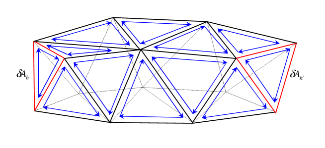
With some additional effort many additional terms can be computed in the strong coupling expansion. In practice the method is generally not really competitive with direct numerical evaluation of the path integral via Monte Carlo methods. But it does provide a new way of looking at the functional integral, and provide the basis for new approaches, such as the large limit to be discussed in the second half of the next section.
III.2.3 Discrete Gravity in the Large-d Limit
In the large- limit the geometric expressions for volume, areas and angles simplify considerably, and as will be shown below one can obtain a number of interesting results for lattice gravity. These can then be compared to earlier investigations of continuum Einstein gravity in the same limit (Strominger, 1981).
Here we will consider a general simplicial lattice in dimensions, made out of a collection of flat -simplices glued together at their common faces so as to constitute a triangulation of a smooth continuum manifold, such as the -torus or the surface of a sphere. Each simplex is endowed with vertices, and its geometry is completely specified by assigning the lengths of its edges. We will label the vertices by and denote the square edge lengths by , … , .
As discussed in Sec. III.1.1, the volume of a -simplex can be computed from the determinant of a matrix,
| (577) |
If one calls the above matrix then previous expression can the re-written as
| (578) |
In general the formulae for volumes and angles are quite complicated and therefore of limited use in large dimensions. The next step consists in expanding them out in terms of small edge length variations, by setting
| (579) |
From now on we will set . Unless stated otherwise, we will be considering the expansion about the equilateral case, and set ; later on this restriction will be relaxed. In the equilateral case one has for the volume of a simplex
| (580) |
From the well-known expansion for determinants
one finds after a little algebra
| (582) |
Note that the terms linear in , which would have required a shift in the ground state value of for non-vanishing cosmological constant , vanish to leading order in . The complete volume term appearing in the action can then be easily written down using the above expressions.
In dimensions the dihedral angle in a -dimensional simplex of volume , between faces of volume and , is obtained from Eq. (340)
| (583) |
In the equilateral case one has for the dihedral angle
| (584) |
which will require four simplices to meet on a hinge, to give a deficit angle of in large dimensions. One notes that in large dimensions the simplices look locally (i.e. at a vertex) more like hypercubes. Several -dimensional simplices will meet on a -dimensional hinge, sharing a common face of dimension between adjacent simplices. Each simplex has edges “on” the hinge, some more edges are then situated on the two “interfaces” between neighboring simplices meeting at the hinge, and finally one edge lies “opposite” to the hinge in question.
In the large limit one then obtains, to leading order for the dihedral angle at the hinge with vertices labelled by
| (585) | |||||
From the expressions in Eq. (582) for the volume and (585) for the dihedral angle one can then evaluate the -dimensional Euclidean lattice action, involving cosmological constant and scalar curvature terms as in Eq. (371)
| (586) |
where is the -dimensional deficit angle, . The lattice functional integral is then
| (587) |
To evaluate the curvature term appearing in the gravitational lattice action one needs the hinge volume , which is easily obtained from Eq. (582), by reducing .
We now specialize to the case where four simplices meet at a hinge. When expanded out in terms of the ’s one obtains for the deficit angle
The action contribution involving the deficit angle is then, for a single hinge,
| (589) |
It involves two types of terms: one linear in the (single) edge opposite to the hinge, as well as a term involving a product of two distinct edges, connecting any hinge vertex to the two vertices opposite to the given hinge. Since there are four simplices meeting on one hinge, one will have 4 terms of the first type, and terms of the second type.
To obtain the total action, a sum over all simplices, resp. hinges, has still to be performed. Dropping the irrelevant constant term and summing over edges one obtains for the total action in the large limit
| (590) |
up to an overall multiplicative factor , which will play no essential role in the following.
The next step involves the choice of a specific lattice. Here we will evaluate the action for the cross polytope . The cross polytope is the regular polytope in dimensions corresponding to the convex hull of the points formed by permuting the coordinates , and has therefore vertices. It is named so because its vertices are located equidistant from the origin, along the Cartesian axes in -space. The cross polytope in dimensions is bounded by -simplices, has vertices and edges.
In three dimensions, it represents the convex hull of the octahedron, while in four dimensions the cross polytope is the 16-cell (Coxeter 1948; Coxeter 1974). In the general case it is dual to a hypercube in dimensions, with the ‘dual’ of a regular polytope being another regular polytope having one vertex in the center of each cell of the polytope one started with. Fig. 28 shows as an example the polytope .

When we consider the surface of the cross polytope in dimensions, we have an object of dimension , which corresponds to a triangulated manifold with no boundary, homeomorphic to the sphere. From Eq. (LABEL:eq:deficit-d) the deficit angle is then given to leading order by
| (591) |
and therefore close to flat in the large limit (due to our choice of an equilateral starting configuration). Indeed if the choice of triangulation is such that the deficit angle is not close to zero, then the discrete model leads to an average curvature whose magnitude is comparable to the lattice spacing or ultraviolet cutoff, which from a physical point of view does not seem very attractive: one obtains a space-time with curvature radius comparable to the Planck length.
When evaluated on such a manifold the lattice action becomes
| (592) |
Dropping the correction the action is proportional to
| (593) |
Since there are edges in the cross polytope, one finds therefore that, at the critical point , the quadratic form in , defined by the above action, develops zero eigenvalues.
This result is quite close to the zero eigenvalues expected in the continuum for large , with the factor of four discrepancy presumably attributed to an underlying intrinsic ambiguity that arises when trying to identify lattice points with points in the continuum.
It is worth noting here that the competing curvature () and cosmological constant () terms will have comparable magnitude when
| (594) |
Here we have further allowed for the possibility that the average lattice spacing is not equal to one (in other words, we have restored the appropriate overall scale for the average edge length, which is in fact largely determined by the value of ).
The average lattice spacing can easily be estimated from the following argument. The volume of a general equilateral simplex is given by Eq. (580), multiplied by an additional factor of . In the limit of small the average volume of a simplex is largely determined by the cosmological term, and can therefore be computed from
| (595) |
with . After doing the integral over with measure and solving this last expression for one obtains
| (596) |
(which, for example, gives for in four dimensions, in reasonable agreement with the actual value found near the transition point).
This then gives for the estimate in , to be compared with obtained in (Hamber, 2000) by direct numerical simulation in four dimensions. Even in one finds again for , from Eqs. (594) and (596), , to be compared with obtained in (Hamber and Williams, 1993) by direct numerical simulation.
Using Eq. (596) inserted into Eq. (594) one obtains in the large limit for the dimensionless combination
| (597) |
To summarize, an expansion in powers of can be developed, which relies on a combined use of the weak field expansion. It can be regarded therefore as a double expansion in and , valid wherever the fields are smooth enough and the geometry is close to flat, which presumably is the case in the vicinity of the lattice critical point at .
A somewhat complementary expansion can be set up, which does not require weak fields, but relies instead on the strong coupling (small , or large ) limit. As such it will be a double expansion in and . Its validity will be in a regime where the fields are not smooth, and in fact will involve lattice field configurations which are very far from smooth at short distances.
The general framework for the strong coupling expansion for pure quantum gravity was outlined in the previous section, and is quite analogous to what one does in gauge theories (Balian, Drouffe and Itzykson, 1975). One expands in powers of as in Eq. (560)
| (598) |
Then one can show that dominant diagrams contributing to correspond to closed surfaces tiled with elementary transport loops. In the case of the hinge-hinge connected correlation function the leading contribution at strong coupling come from closed surfaces anchored on the two hinges, as in Eq. (576).
It will be advantageous to focus on general properties of the parallel transport matrices , discussed previously in Sec. III.1.2. For smooth enough geometries, with small curvatures, these rotation matrices can be chosen to be close to the identity. Small fluctuations in the geometry will then imply small deviations in the ’s from the identity matrix. But for strong coupling () the measure does not significantly restrict fluctuations in the lattice metric field. As a result we will assume that these fields can be regarded, in this regime, as basically unconstrained random variables, only subject to the relatively mild constraints implicit in the measure . The geometry is generally far from smooth since there is no coupling term to enforce long range order (the coefficient of the lattice Einstein term is zero), and one has as a consequence large local fluctuations in the geometry. The matrices will therefore fluctuate with the local geometry, and average out to zero, or a value close to zero. In the sense that, for example, the rotation
| (599) |
averages out to zero when integrated over . In general an element of is described by independent parameters, which in the case at hand can be conveniently chosen as the six Euler angles. The uniform (Haar) measure over the group is then
| (600) |
This is just a special case of the general result, which reads
| (601) |
with , .
These averaging properties of rotations are quite similar of course to what happens in Yang-Mills theories, or even more simply in (compact) QED, where the analogues of the rotation matrices are phase factors . There one has and . In addition, for two contiguous closed paths and sharing a common side one has
| (602) |
with the slightly larger path encircling the two loops. For a closed surface tiled with many contiguous infinitesimal closed loops the last expression evaluates to , due to the divergence theorem. In the lattice gravity case the discrete analog of this last result is considerably more involved, and ultimately represents the (exact) lattice analog of the contracted Bianchi identities. An example of a closed surface tiled with parallel transport polygons (here chosen for simplicity to be triangles) is shown in Fig. 29.
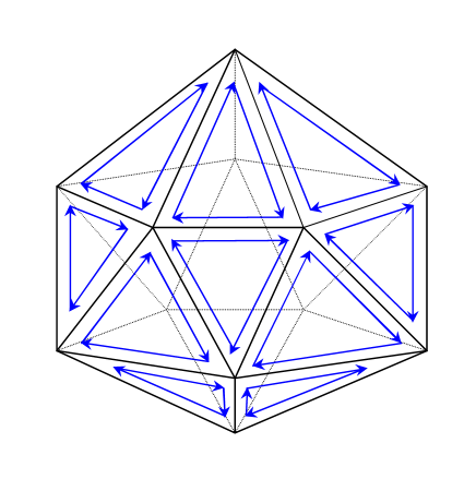
As one approaches the critical point, , one is interested in random surfaces which are of very large extent. Let be the number of polygons in the surface, and set since after all one is describing a surface. The critical point then naturally corresponds to the appearance of surfaces of infinite extent,
| (603) |
A legitimate parallel is to the simpler case of scalar field theories, where random walks of length describing particle paths become of infinite extent at the critical point, situated where the inverse of the (renormalized) mass , expressed in units of the ultraviolet cutoff, diverges.
In the present case of polygonal random surfaces, one can provide the following concise argument in support of the identification in Eq. (603). First approximate the discrete sums over , as they appear for example in the strong coupling expansion for the average curvature, Eq. (561) or its correlation, Eq. (571), by continuous integrals over areas
| (604) |
where is the area of a given surface. The term can be regarded as counting the multiplicity of the surface (its entropy, in statistical mechanics terms). The exponent depends on the specific quantity one is looking at. For the average curvature one has from Eq. (566) , while for its derivative, the curvature fluctuation (the curvature correlation function at zero momentum), one expects . The saddle point is located at
| (605) |
From this discussion one then concludes that close to the critical point very large areas dominate, as claimed in Eq. (603).
Furthermore, one would expect that the universal geometric scaling properties of such a (closed) surface would not depend on its short distance details, such as whether it is constructed out of say triangles or more complex polygons. In general excluded volume effects at finite will provide constraints on the detailed geometry of the surface, but as these constraints can presumably be neglected and one is dealing then with a more or less unconstrained random surface. This should be regarded as a direct consequence of the fact that as there are infinitely many dimensions for the random surface to twist and fold into, giving a negligible contribution from unallowed (by interactions) directions. In the following we will assume that this is indeed the case, and that no special pathologies arise, such as the collapse of the random surface into narrow tube-like, lower dimensional geometric configurations. Then in the large limit the problem simplifies considerably.
Related examples for what is meant in this context are the simpler cases of random walks in infinite dimensions, random polymers and random surfaces in gauge theories (Drouffe, Parisi and Sourlas, 1979), which have been analysed in detail in the large- limit. There too the problem simplifies considerably in such a limit since excluded volume effects (self-intersections) can be neglected there as well. A summary of these results, with a short derivation, is given in the appendices of (Hamber and Williams, 2006).
Following (Gross, 1984) one can define the partition function for such an ensemble of unconstrained random surfaces, and one finds that the mean square size of the surface increases logarithmically with the intrinsic area of the surface. This last result is usually interpreted as the statement that an unconstrained random surface has infinite fractal (or Hausdorff) dimension. Although made of very many triangles (or polygons), the random surface remains quite compact in overall size, as viewed from the original embedding space. In a sense, an unconstrained random surface is a much more compact object than an unconstrained random walk, for which . Identifying the size of the random surface with the gravitational correlation length then gives
| (606) |
From the definition of the exponent , namely , the above result then implies (i.e. a weak logarithmic singularity) at .
It is of interest to contrast the result for gravity in large dimensions with what one finds for scalar (Wilson and Fisher, 1972; Wilson 1973) and gauge (Drouffe, Parisi and Sourlas, 1979) fields, in the same limit . So far, known results can be summarized as follows
| (607) | |||||
It should be regarded as encouraging that the new value obtained here, namely for gravitation, appears to some extent to be consistent with the general trend observed for lower spin, at least at infinite dimension. What happens in finite dimensions? The situation becomes much more complicated since the self-intersection properties of the surface have to be taken into account. But a simple geometric argument then suggests in finite but large dimensions (Hamber and Williams, 2004).
IV NUMERICAL STUDIES IN FOUR DIMENSIONS
The exact evaluation of the lattice functional integral for quantum gravity by numerical methods allows one to investigate a regime which is generally inaccessible by perturbation theory, where the coupling is strong and quantum fluctuations are expected to be large.
The hope in the end is to make contact with the analytic results obtained, for example, in the expansion, and determine which scenarios are physically realized in the lattice regularized model, and then perhaps even in the real world.
Specifically, one can enumerate several major questions that one would like to get at least partially answered.
-
The first one is: which scenarios suggested by perturbation theory are realized in the lattice theory? Perhaps a stable ground state for the quantum theory cannot be found, which would imply that the regulated theory is still inherently pathological.
-
Furthermore, if a stable ground state exists for some range of bare parameters, does it require the inclusion of higher derivative couplings in an essential way, or is the minimal theory, with an Einstein and a cosmological term, sufficient?
-
Does the presence of dynamical matter, say in the form of a massless scalar field, play an important role, or is the non-perturbative dynamics of gravity largely determined by the pure gravity sector (as in Yang-Mills theories)?
-
Is there any indication that the non-trivial ultraviolet fixed point scenario is realized in the lattice theory in four dimensions? This would imply, as in the non-linear sigma model, the existence of at least two physically distinct phases and non-trivial exponents. Which quantity can be used as an order parameter to physically describe, in a qualitative, way the two phases?
-
A clear physical characterization of the two phases would allow one, at least in principle, to decide which phase, if any, could be realized in nature. Ultimately this might or might not be possible based on purely qualitative aspects. As will discussed below, the lattice continuum limit is taken in the vicinity of the fixed point, so close to it is the physically most relevant regime.
-
At the next level one would hope to be able to establish a quantitative connection with those continuum perturbative results which are not affected by uncontrollable errors, such as for example the expansion of Sec. II.3.4. Since the lattice cutoff and the method of dimensional regularization cut the theory off in the ultraviolet in rather different ways, one needs to compare universal quantities which are cutoff-independent. One example is the critical exponent , as well as any other non-trivial scaling dimension that might arise. Within the expansion only one such exponent appears, to all orders in the loop expansion, as . Therefore one central issue in the lattice regularized theory is the value of the universal exponent .
Knowledge of would allow one to be more specific about the running of the gravitational coupling. One purpose of the discussion in Sec. II.3.2 was to convince the reader that the exponent determines the renormalization group running of in the vicinity of the fixed point, as in Eq. (206) for the non-linear -model, and more appropriately in Eq. (298) for quantized gravity. From a practical point of view, on the lattice it is difficult to determine the running of directly from correlation functions , since the effects from the running of are generally small. Instead one would like to make use of the analog of Eqs. (213), (243) and (244) for the non-linear -model, and, again, more appropriately of Eqs. (302) and possibly (308) for gravity to determine , and from there the running of . But the correlation length is also difficult to compute, since it enters the curvature correlations at fixed geodesic distance, which are hard to compute for (genuinely geometric) reasons to be discussed later. Furthermore, these generally decay exponentially in the distance at strong , and can therefore be difficult to compute due to the signal to noise problem of numerical simulations.
Fortunately the exponent can be determined instead, and with good accuracy, from singularities of the derivatives of the path integral , whose singular part is expected, on the basis of very general arguments, to behave in the vicinity of the fixed point as where is the gravitational correlation length. From Eq. (302) relating to and one can then determine , as well as the critical coupling .
IV.1 Observables, Phase Structure and Critical Exponents
The starting point is once again the lattice regularized path integral with action as in Eq. (371) and measure as in Eq. (404). Then the lattice action for pure four-dimensional Euclidean gravity contains a cosmological constant and Regge scalar curvature term as in Eq. (418)
| (608) |
with , and leads to the regularized lattice functional integral
| (609) |
where, as customary, the lattice ultraviolet cutoff is set equal to one (i.e. all length scales are measured in units of the lattice cutoff). The lattice measure is given in Eq. (404) and will be therefore of the form
| (610) |
with a real parameter given below.
Ultimately the above lattice partition function is intended as a regularized form of the continuum Euclidean Feynman path integral of Eq. (182),
| (611) |
with functional measure over the ’s of the form
| (612) |
where is a real parameter constrained by the requirement . For one obtains the De Witt measure of Eq. (166), while for one recovers the original Misner measure of Eq. (170). In the following we will mostly be interested in the four-dimensional case, for which and therefore for the DeWitt measure.
It is possible to add higher derivative terms to the lattice action and investigate how the results are affected. The original motivation was that they would improve the convergence properties of functional integral for the lattice theory, but extensive numerical studies suggest that they don’t seem to be necessary after all. In any case, with such terms included the lattice action for pure gravity aquires the two additional terms whose lattice expressions can be found in Eqs. (439) and (450),
| (613) | |||||
The above action is intended as a lattice form for the continuum action
| (614) |
and is therefore of the form in Eqs. (103) and (451). Because of its relative complexity, in the following the Weyl term will not be considered any further, and will chosen so that . Thus the only curvature term to be discussed here will be a Riemann squared contribution, with a (small) positive coefficient .
IV.1.1 Invariant Local Gravitational Averages
Among the simplest quantum mechanical averages is the one associated with the local curvature
| (615) |
The curvature associated with the quantity above is the one that would be detected when parallel-tranporting vectors around infinitesimal loops, with size comparable to the average lattice spacing . Closely related to it is the fluctuation in the local curvature
| (616) |
The latter is related to the connected curvature correlation at zero momentum
| (617) |
Both and are directly related to derivatives of with respect to ,
| (618) |
and
| (619) |
Thus a divergence or non-analyticity in , as caused for example by a phase transition, is expected to show up in these local averages as well. Note that the above expectation values are manifestly invariant, since they are related to derivatives of .
On the lattice one prefers to define quantities in such a way that variations in the average lattice spacing are compensated by an appropriate factor determined from dimensional considerations. In the case of the average curvature one defines therefore the lattice quantity as
| (620) |
and similarly for the curvature fluctuation,
| (621) |
Fluctuations in the local curvature probe graviton correlations, and are expected to be sensitive to the presence of a massless spin two particle. Note that both of the above expressions are dimensionless, and are therefore unaffected by an overall rescaling of the edge lenghts. As in the continuum, they are proportional to first and second derivatives of with respect to .
One can contrast the behavior of the preceding averages, related to the curvature, with the corresponding quantities involving the local volumes (the quantity in the continuum). Consider the average volume per site
| (622) |
and its fluctuation, defined as
| (623) |
where is the volume associated with the hinge . The last two quantities are again simply related to derivatives of with respect to the bare cosmological constant , as for example in
| (624) |
and
| (625) |
Some useful relations and sum rules can be derived, which follow directly from the scaling properties of the discrete functional integral. Thus a simple scaling argument, based on neglecting the effects of curvature terms entirely (which, as will be seen below, vanish in the vicinity of the critical point), gives an estimate of the average volume per edge [for example from Eqs. (595) and (596)]
| (626) |
where is the functional measure parameter in Eqs. (175) and (404). In four dimensions direct numerical simulations with (corresponding to the lattice DeWitt measure) agree quite well with the above formula.
Some exact lattice identities can be obtained from the scaling properties of the action and measure. The bare couplings and in the gravitational action are dimensionful in four dimensions, but one can define the dimensionless ratio , and rescale the edge lengths so as to eliminate the overall length scale . As a consequence the path integral for pure gravity,
| (627) |
obeys the scaling law
| (628) |
where represents the number of edges in the lattice, and the measure () has been selected. This implies in turn a sum rule for local averages, which for the measure reads
| (629) |
and is easily derived from Eq. (628) and the definitions in Eqs. (618) and (624). represents the number of sites in the lattice, and the averages are defined per site (for the hypercubic lattice divided up into simplices as in Fig. 26, ). This last formula can be very useful in checking the accuracy of numerical evaluations of the path integral. A similar sum rule holds for the fluctuations
| (630) | |||||
In light of the above discussion one can therefore consider without loss of generality the case of unit bare cosmological coupling (in units of the cutoff). Then all lengths are expressed in units of the fundamental microscopic length scale .
IV.1.2 Invariant Correlations at Fixed Geodesic Distance
Compared to ordinary field theories, new issues arise in quantum gravity due to the fact that the physical distance between any two points and
| (631) |
is a fluctuating function of the background metric . In addition, the Lorentz group used to classify spin states is meaningful only as a local concept.
In the continuum the shortest distance between two events is determined by solving the equation of motion (equation of free fall, or geodesic equation)
| (632) |
On the lattice the geodesic distance between two lattice vertices and requires the determination of the shortest lattice path connecting several lattice vertices, and having the two given vertices as endpoints. This can be done at least in principle by enumerating all paths connecting the two points, and then selecting the shortest one. Equivalently it can be computed from the scalar field propagator, as in Eq. (473).
Consequently physical correlations have to be defined at fixed geodesic distance , as in the following correlation between scalar curvatures
| (633) |
Generally these do not go to zero at large separation, so one needs to define the connected part, by subtracting out the value at . These will be indicated in the following by the connected average, and we will write the resulting connected curvature correlation function at fixed geodesic distance compactly as
| (634) |
One can define several more invariant correlation functions at fixed geodesic distance for other operators involving curvatures (Hamber, 1994). The gravitational correlation function just defined is similar to the one in non-Abelian gauge theories, Eq. (327).
In the lattice regulated theory one can define similar correlations, using for example the correspondence of Eqs. (366) or (438) for the scalar curvature
| (635) |
If the deficit angles are averaged over a number of contiguous hinges sharing a common vertex , one is naturally lead to the connected correlation function
| (636) |
which probes correlations in the scalar curvatures. In practice the above lattice correlations have to be computed by a suitable binning procedure: one averages out all correlations in a geodesic distance interval with comparable to one lattice spacing . See Fig. 30. Similarly one can construct the connected correlation functions for local volumes at fixed geodesic distance
| (637) |
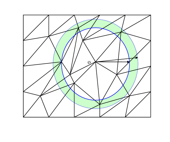
In general one expects for the curvature correlation either a power law decay, for distances sufficiently larger than the lattice spacing ,
| (638) |
with some exponent characterizing the power law decay, or at very large distances an exponential decay, characterized by a correlation length ,
| (639) |
In fact the invariant correlation length is generally defined (in analogy with what one does for other theories) through the long-distance decay of the connected, invariant correlations at fixed geodesic distance . In the pure power law decay case of Eq. (638) the correlation length is of course infinite. One can show from scaling considerations (see below) that the power in Eq. (638) is related to the critical exponent by .
In the presence of a finite correlation length one needs therefore to carefully distinguish between the ”short distance” regime
| (640) |
where Eq. (638) is valid, and the ”long distance” regime
| (641) |
where Eq. (639) is appropriate. Here is the average lattice spacing, and the linear size of the system.
Recently the issue of defining diffeomorphism invariant correlations in quantum gravity has been re-examined from a new perspective (Giddings, Marolf and Hartle, 2006).
IV.1.3 Wilson Lines and Static Potential
In a gauge theory such as QED the static potential can be computed from the manifestly gauge invariant Wilson loop. To this end one considers the process where a particle-antiparticle pair are created at time zero, separated by a fixed distance , and re-annihilated at a later time . In QED the amplitude for such a process associated with the closed loop is given by the Wilson loop
| (642) |
which is a manifestly gauge invariant quantity. Performing the required Gaussian average using the (Euclidean) free photon propagator one obtains
| (643) |
For a rectangular loop of sides and one has after a short calculation
| (644) |
| (645) |
where is an ultraviolet cutoff. In the last line use has been made of the fact that for large imaginary times the exponent in the amplitude involves the energy for the process multiplied by the time . Thus for itself one obtains
| (646) |
which is the correct Coulomb potential for two oppositely charged particles.
To obtain the static potential it is not necessary to consider closed loops. Alternatively, in a periodic box of length one can introduce two long oppositely oriented parallel lines in the time direction, separated by a distance and closed by the periodicity of the lattice, and associated with oppositely charged particles,
| (647) |
In the large time limit one can then show that the result for the potential is the same.
In the gravitational case there is no notion of “oppositely charged particles”, so one cannot use the closed Wilson loop to extract the potential (Modanese 1995). One is therefore forced to consider a process in which one introduces two separate world-lines for the two particles. It is well known that the equation for free fall can be obtained by extremizing the space-time distance travelled. Thus the quantity
| (648) |
can be taken as the Euclidean action contribution associated with the heavy spinless particle of mass .
Next consider two particles of mass , , propagating along parallel lines in the ‘time’ direction and separated by a fixed distance . Then the coordinates for the two particles can be chosen to be with either or . The amplitude for this process is a product of two factors, one for each heavy particle. Each is of the form
| (649) |
where the first argument indicates the spatial location of the Wilson line. For the two particles separated by a distance the amplitude is
| (650) |
For weak fields one sets , with , and therefore . Then the amplitude reduces to
| (651) |
In perturbation theory the averaged amplitude can then be easily evaluated (Hamber and Williams, 1995)
| (652) |
and the static potential has indeed the expected form, . The contribution involving the sum of the two particle masses is independent, and can therefore be subtracted, if the Wilson line correlation is divided by the averages of the individual single line contribution, as in
| (653) |
If one is only interested in the spatial dependence of the potential, one can simplify things further and take . To higher order in the weak field expansion one has to take into account multiple graviton exchanges, contributions from graviton loops and self-energy contributions due to other particles.
How does all this translate to the lattice theory? At this point, the prescription for computing the Newtonian potential for quantum gravity should be clear. For each metric configuration (which is a given configuration of edge lengths on the lattice) one chooses a geodesic that closes due to the lattice periodicity (and there might be many that have this property for the topology of a four-torus), with length (see Fig. 31). One then enumerates all the geodesics that lie at a fixed distance from the original one, and computes the associated correlation between the Wilson lines. After averaging the Wilson line correlation over many metric configurations, one extracts the potential from the dependence of the correlation of Eq. (653). In general since two geodesics will not be at a fixed geodesic distance from each other in the presence of curvature, one needs to introduce some notion of average distance, which then gives the spatial separations of the sources .
On the lattice one can construct the analog of the Wilson line for one heavy particle,
| (654) |
where edges are summed in the “” direction, and the path is closed by the periodicity of the lattice in the direction. One can envision the simplicial lattice as divided up in hypercubes, in which case the points can be taken as the remaining labels for the Wilson line.

For a single line one expects
| (655) |
where is the linear size of lattice in the direction and the renormalized mass. The correlation between Wilson lines at average “distance” is then given by
| (656) |
Numerical studies suggest that the correct qualitative features of the potential emerge close to the critical point. In particular it was found that the potential is attractive close to the critical point, and for two equal mass particles of mass scales, as expected, like the mass squared. As for any correlation in gravity, the accurate determination of the potential as a function of distance is a more difficult task, since at large distance the correlations are small and the statistical noise becomes large. Still, the first results (Hamber and Williams, 1995) suggest that the potential has more or less the expected classical form in the vicinity of the critical point, both as far as the mass dependence and perhaps even the distance dependence are concerned. In particular it is attractive.
The correlation of Wilson lines is not the only possible method to determine that non-perturbative gravity is still attractive. One alternate procedure involves the properties of correlation functions of scalar particles in the presence of gravity (de Bakker and Smit, 1995).
IV.1.4 Scaling in the Vicinity of the Critical Point
In practice the correlation functions at fixed geodesic distance are difficult to compute numerically, and therefore not the best route to study the critical properties. But scaling arguments allow one to determine the scaling behavior of correlation functions from critical exponents characterizing the singular behavior of the free energy and various local averages in the vicinity of the critical point. In general a divergence of the correlation length
| (657) |
signals the presence of a phase transition, and leads to the appearance of a singularity in the free energy . The scaling assumption for the free energy postulates that a divergent correlation length in the vicinity of the critical point at leads to non-analyticities of the type
| (658) | |||||
where the second relationship follows simply from dimensional arguments (the free energy is an extensive quantity). The regular part is generally not determined from by purely dimensional considerations, but as the name implies is a regular function in the vicinity of the critical point. Combining the definition of in Eq. (657) with the scaling assumption of Eq. (658) one obtains
| (659) |
The presence of a phase transition can then be inferred from non-analytic terms in invariant averages, such as the average curvature and its fluctuation. For the average curvature one obtains
| (660) |
up to regular contributions (i.e. constant terms in the vicinity of ). An additive constant can be added, but numerical evidence sor far points to this constant being consistent with zero. Similarly one has for the curvature fluctuation
| (661) |
At a critical point the fluctuation is in general expected to diverge, corresponding to the presence of a divergent correlation length. From such averages one can therefore in principle extract the correlation length exponent of Eq. (657) without having to compute a correlation function.
An equivalent result, relating the quantum expectation value of the curvature to the physical correlation length , is obtained from Eqs. (657) and (660)
| (662) |
again up to an additive constant. Matching of dimensionalities in this last equation is restored by inserting an appropriate power of the Planck length on the r.h.s..
One can relate the critical exponent to the scaling behavior of correlations at large distances. The curvature fluctuation is related to the connected scalar curvature correlator at zero momentum
| (663) |
A divergence in the above fluctuation is then indicative of long range correlations, corresponding to the presence of a massless particle. Close to the critical point one expects for large separations a power law decay in the geodesic distance, as in Eq. (638),
| (664) |
Inserting the above expression in Eq. (663) and comparing with Eq. (661) determines the as . A priori one cannot exclude to possibility that some states acquire a mass away from the critical point, in which case the correlation functions would have the behavior of Eq. (639) for .
IV.1.5 Physical and Unphysical Phases
An important alternative to the analytic methods in the continuum is an attempt to solve quantum gravity directly via numerical simulations. The underlying idea is to evaluate the gravitational functional integral in the discretized theory by summing over a suitable finite set of representative field configurations. In principle such a method given enough configurations and a fine enough lattice can provide an arbitrarily accurate solution to the original quantum gravity theory.
In practice there are several important factors to consider, which effectively limit the accuracy that can be achieved today in a practical calculation. Perhaps the most important one is the enormous amounts of computer time that such calculations can use up. This is particularly true when correlations of operators at fixed geodesic distance are evaluated. Another practical limitation is that one is mostly interested in the behavior of the theory in the vicinity of the critical point at , where the correlation length can be quite large and significant correlations develop both between different lattice regions, as well as among representative field configurations, an effect known as critical slowing down. Finally, there are processes which are not well suited to a lattice study, such as problems with several different length (or energy) scales. In spite of these limitations, the progress in lattice field theory has been phenomenal in the last few years, driven in part by enormous advances in computer technology, and in part by the development of new techniques relevant to the problems of lattice field theories.
The starting point is the generation of a large ensemble of suitable edge length configurations. The edge lengths are updated by a straightforward Monte Carlo algorithm, generating eventually an ensemble of configurations distributed according to the action and measure of Eq. (419) (Hamber and Williams, 1984; Hamber, 1984; Berg, 1985); some more recent references are (Beirl et al, 1994; Riedler et al, 1999; Bittner et al, 2002). Further details of the method as applied to pure gravity can be found for example in the recent work (Hamber, 2000) and will not be repeated here.
As far as the lattice is concerned, one starts with the 4-d hypercube of Fig. 26 divided into simplices, and then stacks a number of such cubes in such a way as to construct an arbitrarily large lattice, as shown in Fig. 32. Other lattice structures are of course possible, including even a random lattice. The expectation is that for long range correlations involving distance scales much larger than the lattice spacing the precise structure of the underlying lattice structure will not matter.
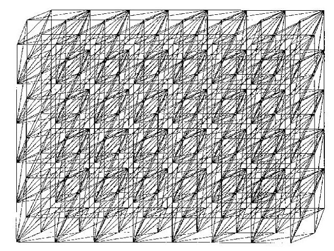
The lattice sizes investigated typically range from sites (3840 edges) to sites (15,728,640 edges). On a dedicated massively parallel supercomputer millions of consecutive edge length configurations can be generated for tens of values of in a few months time.
Even though these lattices are not very large, one should keep in mind that due to the simplicial nature of the lattice there are many edges per hypercube with many interaction terms, and as a consequence the statistical fluctuations can be comparatively small, unless measurements are taken very close to a critical point, and at rather large separation in the case of the correlation functions or the potential. In addition, extrapolations to the infinite volume limit can be aided by finite size scaling methods, which exploit predictable renormalization group properties of finite size systems.
Usually the topology is restricted to a four-torus, corresponding to periodic boundary conditions. One can perform similar calculations with lattices employing different boundary conditions or topology, but one would expect the universal scaling properties of the theory to be determined exclusively by short-distance renormalization effects. Indeed the Feynman rules of perturbation theory do not depend in any way on boundary terms, although some momentum integrals might require an infrared cutoff.
Based on physical considerations it would seem reasonable to impose the constraint that the scale of the curvature be much smaller than the inverse of the average lattice spacing, but still considerably larger than the inverse of the overall system size. Equivalently, that in momentum space physical scales should be much smaller that the ultraviolet cutoff, but much larger than the infrared cutoff. A typical requirement is therefore that
| (665) |
where is the linear size of the system, the correlation length related for example to the large scale curvature by , and the lattice spacing. Contrary to ordinary lattice field theories, the lattice spacing in lattice gravity is a dynamical quantity. Thus the quantity only represents an average cutoff parameter.
Furthermore the bare cosmological constant appearing in the gravitational action of Eq. (419) can be fixed at in units of the cutoff, since it just sets the overall length scale in the problem. The higher derivative coupling can be set to a value very close to since one ultimately is interested in the limit , corresponding to the pure Einstein theory.
One finds that for the measure in Eq. (405) this choice of parameters leads to a well behaved ground state for for higher derivative coupling . The system then resides in the ‘smooth’ phase, with an effective dimensionality close to four. On the other hand for the curvature becomes very large and the lattice collapses into degenerate configurations with very long, elongated simplices. Fig. 33 shows an example of a typical edge length distribution in the well behaved strong coupling phase close to but below .

Fig. 34 shows the corresponding curvature ( or ) distribution.

On one such edge length configuration one can compute the local curvatures, and then project the result on a two-dimensional plane. Using a red color coding for regions of increasingly positive curvature, and a blue color coding for regions of increasingly negative curvature, one obtains the picture in Fig. 35.
One finds that as is varied, the average curvature is negative for sufficiently small (’smooth’ phase), and appears to go to zero continuously at some finite value . For the curvature becomes very large, and the simplices tend to collapse into degenerate configurations with very small volumes (). This ’rough’ or ’collapsed’ phase is the region of the usual weak field expansion (). In this phase the lattice collapses into degenerate configurations with very long, elongated simplices (Hamber, 1984; Hamber and Williams, 1985; Berg, 1985). This phenomenon is usually interpreted as a lattice remnant of the conformal mode instability of Euclidean gravity discussed in Sec. (II.2.4).
An elementary argument can be given to explain the fact that the collapsed phase for has an effective dimension of two. The instability is driven by the Euclidean Einstein term in the action, and in particular its unbounded conformal mode contribution. As the manifold during collapse reaches an effective dimension of two, the action effectively turns into a topological invariant, unable to drive the instability further to a still lower dimension 101010 One way of determining coarse aspects of the underlying geometry is to compute the effective dimension in the scaling regime, for example by considering how the number of points within a thin shell of geodesic distance between and scales with the geodesic distance itself. For distances a few multiples of the average lattice spacing one finds (666) with for (the smooth phase) and for (the rough phase). One concludes that in the rough phase the lattice tends to collapse into a degenerate tree-like configuration, whereas in the smooth phase the effective dimension of space-time is consistent with four. Higher derivative terms affect these results at very short distances, where they tend to make the geometry smoother. .
Accurate and reproducible curvature data can only be obtained for below the instability point, since for an instability develops, presumably associated with the unbounded conformal mode. Its signature is typical of a sharp first order transition, beyond which the system ventually tunnels into the rough, elongated phase which is two-dimensional in nature and has no physically acceptable continuum limit. The instability is caused by the appearance of one or more localized singular configuration, with a spike-like curvature singularity. At strong coupling such singular configurations are suppressed by a lack of phase space due to the functional measure, which imposes non-trivial constraints due to the triangle inequalities and their higher dimensional analogues. In other words, it seems that the measure regulates the conformal instability at sufficiently strong coupling.
As a consequence, the non-analytic behavior of the free energy (and its derivatives, which include for example the average curvature) has to be obtained by analytic continuation of the Euclidean theory into the metastable branch. This procedure, while perhaps unusual, is formally equivalent to the construction of the continuum theory exclusively from its strong coupling (small , large ) expansion
| (667) |
Ultimately it should be kept in mind that one is really only interested in the pseudo-Riemannian case, and not the Euclidean one for which an instability due to the conformal mode is to be expected. Indeed had such an instability not occurred for small enough one might have wondered if the resulting theory still had any relationship to the original continuum theory.
IV.1.6 Numerical Determination of the Scaling Exponents
One way to extract the critical exponent is to fit the average curvature to the form [see Eq. (660)]
| (668) |
Using this set of procedures one obtains on lattices of up to sites and . Note that the average curvature is negative at strong coupling up to the critical point: locally the parallel transport of vectors around infinitesimal loops seems to be described by a lattice version of Euclidean anti-de Sitter space.
Fig. 36 shows as an example a graph of the average curvature raised to the third power. One would expect to get a straight line close to the critical point if the exponent for is exactly . The numerical data indeed supports this assumption, and in fact the linearity of the results close to is quite striking. Using this procedure one obtains on the -site lattice an esimate for the critical point, .

Often it can be advantageous to express results obtained in the cutoff theory in terms of physical (i.e. cutoff independent) quantities. By the latter one means quantities for which the cutoff dependence has been re-absorbed, or restored, in the relevant definition. As an example, an expression equivalent to Eq. (660), relating the vacuum expectation value of the local scalar curvature to the physical correlation length , is
| (669) |
which is obtained by substituting Eq. (657) into Eq. (660). The correct dimensions have been restored in this last equation by supplying appropriate powers of the Planck length , which involves the ultraviolet cutoff . For the result of Eq. (669) becomes particularly simple
| (670) |
Note that a naive estimate based on dimensional arguments would have suggested the incorrect result . Instead the above expression actually vanishes at the critical point. This shows that plays the role of an anomalous dimension, determining the magnitude of deviations from naive dimensional arguments.
Since the critical exponents play such a central role in determining the existence and nature of the continuum limit, it appears desirable to have an independent way of estimating them, which either does not depend on any fitting procedure, or at least analyzes a different and complementary set of data. By systematically studying the dependence of averages on the physical size of the system, one can independently estimate the critical exponents.
Reliable estimates for the exponents in a lattice field theory can take advantage of a comprehensive finite-size analysis, a procedure by which accurate values for the critical exponents are obtained by taking into account the linear size dependence of the result computed in a finite volume .
In practice the renormalization group approach is brought in by considering the behavior of the system under scale transformations. Later the scale dependence is applied to the overall volume itself. The usual starting point for the derivation of the scaling properties is the renormalization group behavior of the free energy
| (671) |
where is the singular, non-analytic part of the free energy, and is the regular part. is the block size in the RG transformation, while and are the relevant eigenvalues of the RG transformation, and the reduced temperature variable that gives the distance from criticality. One denotes here by the relevant eigenvalue, while the remaining eigenvalues are associated with either marginal or irrelevant operators. Usually the leading critical exponent is called , while the next subleading exponent is denoted . For more details on the method we have to refer to the comprehensive review in (Cardy, 1988).
The correlation length determines the asymptotic decay of correlations, in the sense that one expects for example for the two-point function at large distances
| (672) |
The scaling equation for the correlation length itself
| (673) |
implies for that with a correlation length exponent
| (674) |
Derivatives of the free energy with respect to then determine, after setting the scale factor , the scaling properties of physical observables, including corrections to scaling. Thus for example, the second derivative of the free energy with respect to yields the specific heat exponent ,
| (675) |
In the gravitational case one identifies the scaling field with , where involves the bare Newton’s constant. The appearance of singularities in physical averages, obtained from appropriate derivatives of , is rooted in the fact that close to the critical point at the correlation length diverges.
The above results can be extended to the case of a finite lattice of volume and linear dimension . The volume-dependent free energy is then written as
| (676) |
For (a lattice consisting of only one point) one obtains the Finite Size Scaling (FSS) form of the free energy [see for example (Brezin and Zinn-Justin, 1985) for a field-theoretic justification]. After taking derivatives with respect to the fields and , the FSS scaling form for physical observables follows,
| (677) |
where is the scaling dimension of the operator , and an arbitrary function.
As an example, consider the average curvature . From Eq. (677), with and , one has
| (678) |
where is a correction-to-scaling exponent. If scaling involving and holds according to Eq. (677), then all points should lie on the same universal curve.
Fig. 37 shows a graph of the scaled curvature for different values of , versus the scaled coupling . If scaling involving and holds according to Eq. (678), with the scaling dimension for the curvature, then all points should lie on the same universal curve. The data is in good agreement with such behavior, and provides a further test on the exponent, which seems consistent within errors with .

As a second example consider the curvature fluctuation . From the general Eq. (677) one expects in this case, for and ,
| (679) |
where is again a correction-to-scaling exponent. If scaling involving and holds according to Eq. (677), then all points should lie on the same universal curve.
Fig. 38 shows a graph of the scaled curvature fluctuation for different values of , versus the scaled coupling . If scaling involving and holds according to Eq. (679), then all points should lie on the same universal curve. Again the data supports such scaling behavior, and provides a further estimate on the value for .

The value of itself should depend on the size of the system. One expects
| (680) |
where is the infinite-volume limit critical point.
The previous discussion applies to continuous, second order phase transitions. First order phase transitions are driven by instabilities, and are in general not governed by any renormalization group fixed point. The underlying reason is that the correlation length does not diverge at the first order transition point, and thus the system never becomes scale invariant. In the simplest case, a first order transition develops as the system tunnels between two neighboring minima of the free energy. In the metastable branch the free energy acquires a small complex part with a very weak essential singularity in the coupling at the first order transition point (Langer, 1967; Fisher, 1967; Griffiths, 1969). As a consequence, such a singularity is not generally visible from the stable branch, in the sense that a power series expansion in the temperature is unaffected by such a weak singularity. Indeed in the infinite volume limit the singularities associated with a first order transition at become infinitely sharp, a - or -function type singularity. While the singularity in the free energy at the endpoint of the metastable branch (at say ) cannot be explored directly, it can be reached by a suitable analytic continuation from the stable side of the free energy branch. A similar situation arises in the case of lattice with fermions, where zero fermion mass (chiral) limit is reached by extrapolation (Hamber and Parisi, 1983).
From the best data (with the smallest statistical uncertainties and the least systematic effects) one concludes
| (681) |
which suggests for pure quantum gravity. Note that at the critical point the gravitational coupling is not weak, in units of the ultraviolet cutoff. It seems that the value does not correspond to any known field theory or statistical mechanics model in four dimensions. For a perhaps related system, namely dilute branched polymers, it is known that in three dimensions, and at the upper critical dimension , so one would expect a value close to somewhere in between. On the other hand for a scalar field one would have obtained in and for , which seems excluded.
| Method | in | in |
| lattice | 1.67(6) | - |
| lattice | - | 2.98(7) |
| 1.6 | 4.4 | |
| truncation | 1.2 | 2.666 |
| exact ? | 1.5882 | 3 |
Table I: Direct determinations of the critical exponent for quantum gravitation, using various analytical and numerical methods in three and four space-time dimensions.
Table I provides a short summary of the critical exponents for quantum gravitation as obtained by various perturbative and non-perturbative methods in three and four dimensions. The and the truncation method results were discussed previously in Secs. II.3.4 and II.3.5, respectively. The lattice model of Eq. (419) in four dimensions gives for the critical point in units of the ultraviolet cutoff, and which is used for comparison in Table I. In three dimensions the numerical results are consistent with the universality class of the interacting scalar field. The same set of results are compared graphically in Fig. 39 and Fig. 40 below.
The direct numerical determinations of the critical point in and space-time dimensions are in fact quite close to the analytical prediction of the lattice expansion given previously in Eq. (597),
| (682) |
The above expression gives for a bare cosmological constant the estimate in , to be compared with the numerical result in (Hamber, 2000). Even in one has , to be compared with the direct determination from (Hamber and Williams, 1993). These estimates are compared below in Fig. 40.
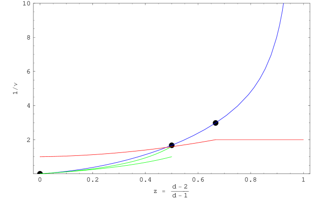
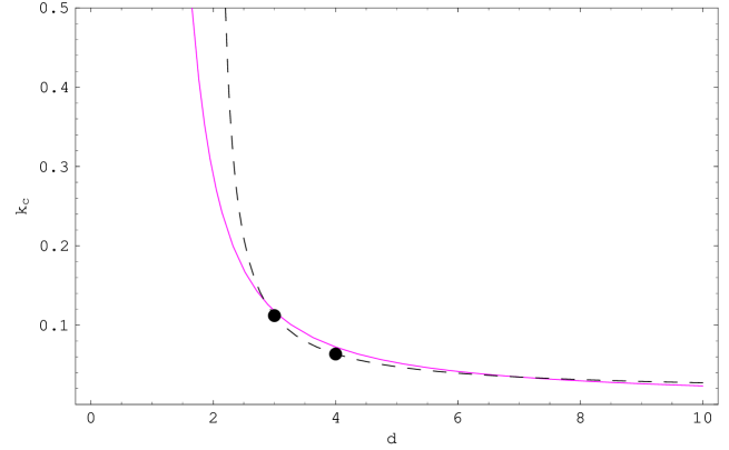
IV.1.7 Renormalization Group and Lattice Continuum Limit
The discussion in the previous sections points to the existence of a phase transition in the lattice gravity theory, with divergent correlation length in the vicinity of the critical point, as in Eq. (657)
| (683) |
As described previously, the existence of such a correlation length is usually inferred indirectly by scaling arguments, from the presence of singularities in the free energy as a function of the lattice coupling . Equivalently, could have been computed directly from correlation functions at fixed geodesic distance using the definition in Eq. (639), or even from the correlation of Wilson lines associated with the propagation of two heavy spinless particles. The outcome of such large scale numerical calculations is eventually a determination of the quantities , and from first principles, to some degree of numerical accuracy.
In either case one expects the scaling result of Eq. (683) close to the fixed point, which we choose to rewrite here in terms of the inverse correlation length
| (684) |
Note that in the above expression the correct dimension for (inverse length) has been restored by inserting explicitly on the r.h.s. the ultraviolet cutoff . Here and are of course still dimensionless quantities, and correspond to the bare microscopic couplings at the cutoff scale, . is a calculable numerical constant, related to in Eq. (657) by . It is worth pointing out that the above expression for is almost identical in structure to the one for the non-linear -model in the expansion, Eq. (220) and in the large limit, Eqs. (243), (244) and (248). It is of course also quite similar to result for continuum gravity, Eq. (302).
The lattice continuum limit corresponds to the large cutoff limit taken at fixed ,
| (685) |
which shows that the continuum limit is reached in the vicinity of the ultraviolet fixed point. Phrased equivalently, one takes the limit in which the lattice spacing is sent to zero at fixed , which requires an approach to the non-trivial UV fixed point . The quantity is supposed to be a renormalization group invariant, a physical scale independent of the scale at which the theory is probed. In practice, since the cutoff ultimately determines the physical value of Newton’s constant , cannot be taken to . Instead a very large value will suffice, , for which it will still be true that which is all that is required for the continuum limit.
For discussing the renormalization group behavior of the coupling it will be more convenient to write the result of Eq. (684) directly in terms of Newton’s constant as
| (686) |
with the dimensionless constant related to by . Note that the above expression only involves the dimensionless ratio , which is the only relevant quantity here. The lattice theory in principle completely determines both the exponent and the amplitude for the quantum correction. Thus from the knowledge of the dimensionless constant in Eq. (684) one can estimate from first principles the value of in Eqs. (691). Lattice results for the correlation functions at fixed geodesic distance give a value for with a significant uncertainty, which, when combined with the values and given above, gives . The rather surprisingly large value for appears here as a consequence of the relatively small value of the lattice in four dimensions.
The renormalization group invariance of the physical quantity requires that the running gravitational coupling varies in the vicinity of the fixed point in accordance with the above equation, with , where is now an arbitrary scale,
| (687) |
The latter is equivalent to the renormalization group invariance requirement
| (688) |
provided is varied in a specific way. Indeed this type of situation was already encountered before, for example in Eqs. (246) and (303). Eq. (688) can therefore be used to obtain, if one so wishes, -function for the coupling in units of the ultraviolet cutoff,
| (689) |
with given in the vicinity of the non-trivial fixed point, using Eq. (687), by
| (690) |
The above procedure is in fact in complete analogy to what was done for the non-linear -model, for example in Eq. (248). But the last two steps are not really necessary, for one can obtain the scale dependence of the gravitational coupling directly from Eq. (687), by simply solving for ,
| (691) |
This last expression can be compared directly to the result of Eq. (298), as well as to the -model result of Eq. (206). The physical dimensions of can be restored by multiplying the above expression on both sides by the ultraviolet cutoff , if one so desires. One concludes that the above result physically implies gravitational anti-screening: the gravitational coupling increases with distance.
Note that the last equation only involves the dimensionless ratio , and is therefore unaffected by whether the coupling is dimensionful (after inserting an appropriate power of the cutoff ) or dimensionless. It simply relates the gravitational coupling at one scale to the coupling at a different scale,
| (692) |
In conclusion, the lattice result for in Eq. (691) and the -function in Eq. (690) are qualitatively similar to what one finds both in the expansion for gravity and in the non-linear -model in the strong coupling phase.
But there are also significant differences. Besides the existence of a phase transition between two geometrically rather distinct phases, one major new aspect provided by non-perturbative lattice studies is the fact that the weakly coupled small phase turns out to be pathological, in the sense that the theory becomes unstable, with the four-dimensional lattice collapsing into a tree-like two-dimensional structure for . While in continuum perturbation theory both phases, and therefore both signs for the coupling constant evolution in Eq. (295), seem acceptable (giving rise to both a “Coulomb” phase, and a strong coupling phase), the Euclidean lattice results rule out the small branched polymer phase. The collapse eventually stops at because the gravitational action then becomes a topological invariant.
It appears difficult therefore to physically characterize the weak coupling phase based on just the lattice results, which only seem to make sense in the strong coupling phase . One could envision an approach wherein such a weak coupling phase would be discussed in the framework of some sort of analytic continuation from the strong coupling phase, which would seem possible at least for some lattice results, such as the gravitational -function of Eq. (690). The latter clearly makes sense on both sides of the transition, just as is the case for Eq. (248) for the non-linear -model. In particular Eq. (690) implies that the coupling will flow towards the Gaussian fixed point for . The scale dependence in this phase will be such that one expects gravitational screening: the coupling gets increasingly weaker at larger distances. But how to remove the geometric collapse to a two-dimensional manifold remains a major hurdle; one could envision an approach where one introduces one more cutoff on the edges at short distances, so that each simplex cannot go below a certain fatness. But if the results so far can be used as a guide, the gradual removal of such a cutoff would then plunge the theory back into a degenerate two-dimensional, and therefore physically unacceptable, geometry.
IV.1.8 Curvature Scales
As can be seen from Eqs. (263) and (628) the path integral for pure quantum gravity can be made to depend on the gravitational coupling and the cutoff only: by a suitable rescaling of the metric, or the edge lengths in the discrete case, one can set the cosmological constant to unity in units of the cutoff. The remaining coupling should then be viewed more appropriately as the gravitational constant in units of the cosmological constant .
The renormalization group running of in Eq. (691) involves an invariant scale . At first it would seem that this scale could take any value, including very small ones based on the naive estimate , which would preclude any observable quantum effects in the foreseeable future. But the result of Eqs. (669) and (670) suggest otherwise, namely that the non-perturbative scale is in fact related to curvature. From astrophysical observation the average curvature is very small, so one would conclude from Eq. (670) that is very large, and possibly macroscopic. But the problem with Eq. (670) is that it involves the lattice Ricci scalar, a quantity related curvature probed by parallel transporting vectors around infinitesimal loops with size comparable to the lattice cutoff . What one would like is instead a relationship between and quantities which describe the geometry on larger scales.
In many ways the quantity of Eq. (687) behaves as a dynamically generated mass scale, quite similar to what happens in the non-linear -model case [Eq. (244)], or in the gravity case [Eq. (299)]. Indeed in the weak field expansion, presumably appropriate for slowly varying fields on very large scales, a mass-like term does appear, as in Eq. (64), with where is the scaled cosmological constant. From the classical field equation one can relate the above , and therefore the mass-like parameter , to curvature, which leads to the identification
| (693) |
with the observed small but non-vanishing cosmological constant.
A further indication that the identification of the observed scaled cosmological constant with a mass-like - and therefore renormalization group invariant - term makes sense beyond the weak field limit can be seen for example by comparing the structure of the three classical field equations
| (694) |
for gravity, QED (massive via the Higgs mechanism) and a self-interacting scalar field, respectively.
A third argument suggesting the identification of the scale with large scale curvature and therefore with the observed scaled cosmological constant goes as follows. Observationally the curvature on large scale can be determined by parallel transporting vectors around very large loops, with typical size much larger than the lattice cutoff . In gravity, curvature is detected by parallel transporting vectors around closed loops. This requires the calculation of a path dependent product of Lorentz rotations , in the Euclidean case elements of , as discussed in Sec. III.1.2. On the lattice, the above rotation is directly related to the path-ordered () exponential of the integral of the lattice affine connection via
| (695) |
Now, in the strongly coupled gravity regime () large fluctuations in the gravitational field at short distances will be reflected in large fluctuations of the matrices. Deep in the strong coupling regime it should be possible to describe these fluctuations by a uniform (Haar) measure. Borrowing from the analogy with Yang-Mills theories, and in particular non-Abelian lattice gauge theories with compact groups [see Eq. (326)], one would therefore expect an exponential decay of near-planar Wilson loops with area of the type
| (696) |
where is the minimal physical area spanned by the near-planar loop. A derivation of this standard result for non-Abelian gauge theories can be found, for example, in the textbook (Peskin and Schroeder, 1995).
In summary, the Wilson loop in gravity provides potentially a measure for the magnitude of the large-scale, averaged curvature, operationally determined by the process of parallel-transporting test vectors around very large loops, and which therefore, from the above expression, is computed to be of the order . One would expect the power to be universal, but not the amplitude, leaving open the possibility of having both de Sitter or anti-de Sitter space at large distances (as discussed previously in Sec. IV.1.6, the average curvature describing the parallel transport of vectors around infinitesimal loops is described by a lattice version of Euclidean anti-de Sitter space). A recent explicit lattice calculation indeed suggests that the de Sitter case is singled out, at least for sufficiently strong copuling (Hamber and Williams, 2007). Furthermore one would expect, based on general scaling arguments, that such a behavior would persists throughout the whole strong coupling phase , all the way up to the on-trivial fixed point. From it then follows the identification of the correlation length with a measure of large scale curvature, the most natural candidate being the scaled cosmological constant , as in Eq. (693). This relationship, taken at face value, implies a very large, cosmological value for , given the present bounds on . Other closely related possibilities may exist, such as an identification of with the Hubble constant (as measured today), determining the macroscopic expansion rate of the universe via the correspondence . Since this quantity is presumably time-dependent, a possible scenario would be one in which , with , for which the horizon radius is .
Since, as pointed out in Sec. II.3.4 and Sec. IV.1.1, the gravitational path integral only depends in a non-trivial way on the dimensionless combination , the physical Newton’s constant itself can be decomposed into non-running and running parts as
| (697) |
where we have used . The running of the second, dimensionless term in square brackets can be directly deduced from either Eqs. (687) or (691). Note that there does not appear there explicitly, since originally it was set equal to one by scaling the metric (or the edge lengths).
IV.1.9 Gravitational Condensate
In strongly coupled gravity there appears to be a deep relationship, already encountered previously in non-Abelian gauge theories, between the non-perturbative scale appearing in Eqs. (691), and the non-perturbative vacuum condensate of Eqs. (669) and (693), which is a measure of curvature. The inescapable conclusion of the results of Eqs. (669) and (395) is that the scale appearing in Eq. (691) is related to curvature, and must be macroscopic for the lattice theory to be consistent. How can quantum effects propagate to such large distances and give such drastic modifications to gravity? The answer to this paradoxical question presumably lies in the fact that gravitation is carried by a massless particle whose interactions cannot be screened, on any length scale.
It is worth pointing out here that the gravitational vacuum condensate, which only exists in the strong coupling phase , and which is proportional to the curvature, is genuinely non-perturbative. One can summarize the result of Eq. (693) as
| (699) |
where the condensate is, according to Eq. (686), non-analytic at . A graviton vacuum condensate of order is of course extraordinarily small compared to the QCD color condensate () and the electro-weak Higgs condensate (). One can pursue the analogy with non-Abelian gauge theories further by stating that the quantum gravity theory cannot provide a value for the non-perturbative curvature scale : it needs to be fixed by some sort of phenomenological input, either by Eq. (691) or by Eq. (693). But one important message is that the scale in those two equations is one and the same.
Can the above physical picture be used to provide further insight into the nature of the phase transition, and more specifically the value for ? We will mention here a simple geometric argument which can be given to support the exact value for pure gravity (Hamber and Williams, 2004). First one notices that the vacuum polarization induced scale dependence of the gravitational coupling as given in Eq. (691) implies the following general structure for the quantum corrected static gravitational potential,
| (700) |
for a point source of mass located at the origin and for intermediate distances . One can visualize the above result by stating that virtual graviton loops cause an effective anti-screening of the primary gravitational source , giving rise to a quantum correction to the potential proportional to . But only for can the additional contribution be interpreted as being due to a close to uniform mass distribution surrounding the original source, of strength
| (701) |
Such a simple geometric interpretation fails unless the exponent for gravitation is exactly one third. In fact in dimensions one would expect based on the geometric argument that if the quantum correction to the gravitational potential arises from such a virtual graviton cloud. These arguments rely of course on the lowest order result for single graviton exchange in dimensions.
Equivalently, the running of can be characterized as being in part due to a tiny non-vanishing (and positive) non-perturbative gravitational vacuum contribution to the cosmological constant, with
| (702) |
and therefore an associated effective classical average curvature of magnitude . It is amusing that for a very large mass distribution , the above expression for the curvature can only be reconciled with the naive dimensional estimate , provided for the gravitational coupling itself one has , which is reminiscent of Mach’s principle and its connection with the Lense-Thirring effect (Lense and Thirring, 1918; Sciama, 1953; Feynman, 1962).
V SCALE DEPENDENT GRAVITATIONAL COUPLING
Non-perturbative studies of quantum gravity suggest the possibility that gravitational couplings might be weakly scale dependent due to nontrivial renormalization group effects. This would introduce a new gravitational scale, unrelated to Newton’s constant, required in order to parametrize the gravitational running in the infrared region. If one is willing to accept such a scenario, then it seems difficult to find a compelling theoretical argument for why the non-perturbative scale entering the coupling evolution equations should be very small, comparable to the Planck length. One possibility is that the relevant non-perturbative scale is related to the curvature and therefore macroscopic in size, which could have observable consequences. One key ingredient in this argument is the relationship, in part supported by Euclidean lattice results combined with renormalization group arguments, between the scaling violation parameter and the scale of the average curvature.
V.1 Effective Field Equations
V.1.1 Scale Dependence of
To summarize the results of the previous section, the result of Eq. (691) implies for the running gravitational coupling in the vicinity of the ultraviolet fixed point
| (703) |
with , and . Since is expected to be very large, the quantity in the above expression should now be identified with the laboratory scale value . Quantum corrections on the r.h.s are therefore quite small as long as , which in real space corresponds to the “short distance” regime .
The interaction in real space is often obtained by Fourier transform, and the above expression is singular as . The infrared divergence needs to be regulated, which can be achieved by utilizing as the lower limit of momentum integration . Alternatively, as a properly infrared regulated version of the above expression one can use
| (704) |
The last form for will only be necessary in the regime where is small, so that one can avoid unphysical results. From Eq. (704) the gravitational coupling then approaches at very large distances the finite value . Note though that in Eqs. (703) or (704) the cutoff no longer appear explicitly, it is absorbed into the definition of . In the follwing we will be mostly interested in the regime , for which Eq. (703) is completely adequate.
The first step in analyzing the consequences of a running of is to re-write the expression for in a coordinate-independent way. The following methods are not new, and have found over the years their fruitful application in gauge theories and gravity, for example in the discussion of non-local effective actions (Vilkovisky, 1984; Barvinsky and Vilkovisky, 1985). Since in going from momentum to position space one usually employs , to obtain a quantum-mechanical running of the gravitational coupling one should make the replacement
| (705) |
and therefore from Eq. (703)
| (706) |
In general the form of the covariant d’Alembertian operator depends on the specific tensor nature of the object it is acting on,
| (707) |
Only on scalar functions one has the fairly simple result
| (708) |
whereas on second rank tensors one has the already significantly more complicated expression .
The running of is expected to lead to a non-local gravitational action, for example of the form
| (709) |
Due to the fractional exponent in general the covariant operator appearing in the above expression, namely
| (710) |
has to be suitably defined by analytic continuation from positive integer powers. The latter can be done for example by computing for positive integer and then analytically continuing to . Alternatively one can make use of the identity
| (711) |
and later perform the relevant integrals with . Other procedures can be used to define , for example based on an integral representation involving the scalar propagator (Lopez Nacir and Mazzitelli, 2007).
It should be stressed here that the action in Eq. (709) should be treated as a classical effective action, with dominant radiative corrections at short distances () already automatically built in, and for which a restriction to generally smooth field configurations does make some sense. In particular one would expect that in most instances it should be possible, as well as meaningful, to neglect terms involving large numbers of derivatives of the metric in order to compute the effects of the new contributions appearing in the effective action.
Had one not considered the action of Eq. (709) as a starting point for constructing the effective theory, one would naturally be led (following Eq. (705)) to consider the following effective field equations
| (712) |
the argument again being the replacement . Being manifestly covariant, these expressions at least satisfy some of the requirements for a set of consistent field equations incorporating the running of . The above effective field equation can in fact be re-cast in a form similar to the classical field equations
| (713) |
with defined as an effective, or gravitationally dressed, energy-momentum tensor. Just like the ordinary Einstein gravity case, in general might not be covariantly conserved a priori, , but ultimately the consistency of the effective field equations demands that it be exactly conserved, in consideration of the Bianchi identity satisfied by the Riemann tensor (a similar problem arises in other non-local modifications of gravity (Barvinsky, 2003)). The ensuing new covariant conservation law
| (714) |
can be then be viewed as a constraint on (or ) which, for example, in the specific case of a perfect fluid, will imply again a definite relationship between the density , the pressure and the RW scale factor , just as it does in the standard case. Then the requirement that the bare energy momentum-tensor be conserved would imply that the quantum contribution itself be separately conserved. That this is indeed attainable can be shown in a few simple cases, such as the static isotropic solution discussed below. There a ”vacuum fluid” is introduced to account for the vacuum polarization contribution, whose energy momentum tensor can be shown to be covariantly conserved. That the procedure is consistent in general is not clear, in which case the present approach should perhaps be limited to phenomenological considerations.
Let us make a few additional comments regarding the above effective field equations, in which we will set the cosmological constant from now on. One simple observation is that the trace equation only involves the (simpler) scalar d’Alembertian, acting on the trace of the energy-momentum tensor
| (715) |
Finally, to the order one is working here, the above effective field equations should be equivalent to
| (716) |
where the running of has been moved over to the “gravitational” side.
V.1.2 Poisson’s Equation and Vacuum Polarization Cloud
One of the simplest cases to analyze is of course the static case. The non-relativistic, static Newtonian potential is defined as usual as
| (717) |
and therefore proportional to the Fourier transform of
| (718) |
But, as already mentioned, for small proper care has to be exercised in providing a properly infrared regulated version of the above expression, which, from Eq. (704), reads
| (719) |
where the limit should be taken at the end of the calculation.
Given the running of from either Eq. (704), or Eq. (703) in the large limit, the next step is naturally an attempt at finding a solution to Poisson’s equation with a point source at the origin, so that one can determine the structure of the quantum corrections to the static gravitational potential in real space. There are in principle two equivalent ways to compute the potential , either by inverse Fourier transform of Eq. (718), or by solving Poisson’s equation with the source term given by the inverse Fourier transform of the correction to , as given below in Eq. (722). The zero-th order term then gives the standard Newtonian term, while the correction in general is given by a rather complicated hypergeometric function. But for the special case the Fourier transform of Eq. (719) is easy to do, the integrals are elementary and the running of so obtained is particularly transparent,
| (720) |
where we have set and . therefore increases slowly from its value at small to the larger value at infinity. Fig. 41 illustrates the anti-screening effect of the virtual graviton cloud. Fig. 42 gives a schematic illustration of the behavior of as a function of .

Another possible procedure to obtain the static potential is to solve directly the radial Poisson equation for . This will give a density which can later be used to generalize to the relativistic case. In the case one needs to solve , or in the radial coordinate for
| (721) |
with the source term determined from the inverse Fourier transform of the correction term in Eq. (719). The latter is given by
| (722) |
with the constant
| (723) |
One can verify that the vacuum polarization density has the property
| (724) |
where the standard integral has been used. Note that the gravitational vacuum polarization distribution is singular close to , just as in QED, Eq. (319).
The result for (discussed in the following, as an example, for ) can then be obtained by solving the radial equation for ,
| (725) |
where the (modified) Bessel function is expanded out to lowest order in , , giving
| (726) |
where the two integration constants are matched to the general large solution
| (727) |
with . Note again that the vacuum polarization density has the expected normalization property
| (728) |
so that the total enclosed additional gravitational charge is indeed just , and .
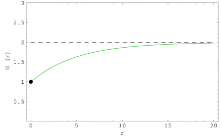
V.1.3 Static Isotropic Solution
The discussion of the previous section suggests that the quantum correction due to the running of can be described, at least in the non-relativistic limit of Eq. (704) as applied to Poisson’s equation, in terms of a vacuum energy density , distributed around the static source of strength in accordance with the result of Eqs. (722) and Eq. (724).
In general a manifestly covariant implementation of the running of , via the given in Eq. (706), will induce a non-vanishing effective pressure term. It is natural therefore to attempt to represent the vacuum polarization cloud by a relativistic perfect fluid, with energy-momentum tensor
| (729) |
which in the static isotropic case reduces to
| (730) |
and gives a trace . The , and components of the field equations then read
| (731) |
| (732) |
| (733) |
with the component equal to times the component. Covariant energy conservation implies
| (734) |
and forces a definite relationship between , and . The three field equations and the energy conservation equation are, as usual, not independent, because of the Bianchi identity. It seems reasonable to attempt to solve the above equations (usually considered in the context of relativistic stellar structure (Misner Thorne Wheeler 1972)) with the density given by the of Eq. (722). This of course raises the question of how the relativistic pressure should be chosen, an issue that the non-relativistic calculation did not have to address. One finds that covariant energy conservation in fact completely determines the pressure in the static case, leading to consistent equations and solutions (note that in particular it would not be consistent to take ).
Since the function drops out of the field equation, the latter can be integrated immediately, giving
| (735) |
It is natural to identify , which of course corresponds to the solution with (). Next, the field equation can be solved for ,
| (736) |
with the constant again determined by the requirement that the above expression for reduce to the standard Schwarzschild solution for (), giving . The last task left therefore is the determination of the pressure . One needs to solve the equation
| (737) |
which is usually referred to as the equation of hydrostatic equilibrium. From now on we will focus only the case . The last differential equation can be solved for ,
| (738) |
where the constant of integration has to be chosen so that when (no quantum correction) one has as well. Because of the singularity in the integrand at , we will take the lower limit in the integral to be , with .
To proceed further, one needs the explicit form for , which was given in Eq. (722),
| (739) |
The required integrands involve for general the modified Bessel function , which can lead to rather complicated expressions for the general case. To determine the pressure, one supposes that it as well has a power dependence on in the regime under consideration, , where is a numerical constant, and then substitute into the pressure equation Eq. (737). This gives, past the horizon the algebraic condition
| (740) |
giving the same power as for , and surprisingly also , implying that in this regime only gives a consistent solution.
The case can be dealt with separately, starting from the expression for for
| (741) |
One has for small
| (742) |
and consequently
| (743) |
From Eq. (737) one can then obtain an expression for the pressure , and one finds again in the limit
| (744) |
After performing the required integral in Eq. (736), and evaluating the resulting expression in the limit , one obtains
| (745) |
It is encouraging to note that in the solution just obtained the running of is the same in and . The expressions for and are consistent with a gradual slow increase in with distance, in accordance with the formula
| (746) |
in the regime , and therefore of course in agreement with the original result of Eqs. (703) or (704), namely that the classical laboratory value of is obtained for . Note that the correct relativistic small correction of Eq. (746) agrees roughly in magnitude (but not in sign) with the approximate non-relativistic, Poisson equation result of Eq. (726).
There are similarities, as well as some rather substantial differences, with the corresponding QED result of Eq. (319). In the gravity case, the correction vanishes as goes to zero: in this limit one is probing the bare mass, unobstructed by its virtual graviton cloud. On the other hand, in the QED case, as one approaches the source one is probing the bare charge, whose magnitude diverges logarithmically for small .
Finally it should be recalled that neither function or are directly related to the relativistic potential for particle orbits, which is given instead by the combination
| (747) |
where is proportional to the orbital angular momentum of the test particle, as discussed for example in (Hartle 2005).
The running term acts in a number of ways as a local cosmological constant term, for which the dependence of the vacuum solution for small is fixed by the nature of the Schwarzschild solution with a cosmological constant term. One can therefore wonder what the solutions might look like in dimensions. In dimensions the Schwarzschild solution to Einstein gravity with a cosmological term is (Myers and Perry 1986)
| (748) |
with , which would suggest, in analogy with the results for given above that in dimensions only is possible. This last result would also be in agreement with the exact value found at in Sec. III.2.3.
V.1.4 Cosmological Solutions
A scale dependent Newton’s constant will lead to small modifications of the standard cosmological solutions to the Einstein field equations. Here we will provide a brief discussion of what modifications are expected from the effective field equations on the basis of , as given in Eq. (705), which itself originates in Eqs. (704) and (703).
One starts therefore from the quantum effective field equations of Eq. (712),
| (749) |
with defined in Eq. (710). In the Friedmann-Robertson-Walker (FRW) framework these are applied to the standard homogeneous isotropic metric
| (750) |
It should be noted that there are two quantum contributions to the above set of effective field equations. The first one arises because of the presence of a non-vanishing cosmological constant caused by the non-perturbative vacuum condensate of Eq. (693). As in the case of standard FRW cosmology, this is expected to be the dominant contributions at large times , and gives an exponential (for or cyclic (for ) expansion of the scale factor.
The second contribution arises because of the running of in the effective field equations,
| (751) |
for , with and a calculable coefficient of order one [see Eqs. (703) and (704)].
As a first step in solving the new set of effective field equations, consider first the trace of the field equation in Eq. (749), written as
| (752) |
where is the scalar curvature. Here the operator has been moved over on the gravitational side, so that it now acts on functions of the metric only, using the binomial expansion of . To proceed further, one needs to compute the effect of on the scalar curvature. The d’Alembertian operator acting on scalar functions is given by
| (753) |
and for the Robertson-Walker metric, acting on functions of only, one obtains a fairly simple result in terms of the scale factor
| (754) |
As a next step one computes the action of on the scalar curvature , which gives
| (755) |
and then on etc. Since the resulting expressions are of rapidly escalating complexity, one sets , in which case one has first for the scalar curvature itself
| (756) |
Acting with on the above expression gives for and arbitrary power
| (757) |
with the coefficient given by
| (758) |
Here use has been made of the relationship
| (759) |
to analytically continue the above expressions to negative fractional (Samko et al 1993; Zavada 1998). For the correction on the scalar curvature term is therefore of the form
| (760) |
with
| (761) |
Putting everything together, one then obtains for the trace part of the effective field equations
| (762) |
The new term can now be moved back over to the matter side in accordance with the structure of the original effective field equation of Eq .(749), and thus avoids the problem of having to deal with the binomial expansion of . One then has
| (763) |
which is the Robertson-Walker metric form of Eq. (749). If one assumes for the matter density , then matching powers when the new term starts to take over at larger distances gives the first result
| (764) |
Thus the density decreases faster in time than the classical value would indicate. The expansion appears therefore to be accelerating, but before reaching such a conclusion one needs to determine the time dependence of the scale factor (or ) as well.
One can alternatively pursue the following exercise in order to check the overall consistency of the approach. Consider acting on instead, as in the trace of the effective field equation Eq. (749)
| (765) |
for and . For and one finds in this case
| (766) |
which again implies for the value as in Eq. (764) for large(r) times, when the quantum correction starts to become important (since the left hand side of Einstein’s equation always goes like , no matter what the value for is, at least for k=0).
The next step is to examine the full effective field equations (as opposed to just their trace part) of Eq. (715) with cosmological constant ,
| (767) |
Here the d’Alembertian operator
| (768) |
acts on a second rank tensor,
| (769) |
and would thus seem to require the calculation of 1920 terms, of which fortunately many vanish by symmetry. Next one assumes again that has the perfect fluid form, for which one obtains from the action of on
| (770) |
with the remaining components equal to zero. Note that a non-vanishing pressure contribution is generated in the effective field equations, even if one assumes initially a pressureless fluid, . As before, repeated applications of the d’Alembertian to the above expressions leads to rapidly escalating complexity, which can only be tamed by introducing some further simplifying assumptions. In the following we will therefore assume that has the perfect fluid form appropriate for non-relativistic matter, with a power law behavior for the density, , and . Thus all components of vanish in the fluid’s rest frame, except the one, which is simply . Setting and one then finds
| (771) |
which again shows that the and components get mixed by the action of the operator, and that a non-vanishing component gets generated, even though it was not originally present.
Higher powers of the d’Alembertian acting on can then be computed as well. But a comparison with the left hand (gravitational) side of the effective field equation, which always behaves like for , shows that in fact a solution can only be achieved at order provided the exponent satisfies , or
| (772) |
as was found previously from the trace equation, Eqs. (749) and (764). As a result one obtains a much simpler set of expressions, which for general read
| (773) |
for the component, and similarly for the component
| (774) |
But remarkably one finds for the two coefficients the simple identity
| (775) |
as well as and . The identity implies, from the consistency of the and effective field equations at large times,
| (776) |
One can find a closed form expression for the coefficients and as functions of which are not particularly illuminating, except for providing an explicit proof that they exist.
As a result, in the simplest case, namely for a universe filled with non-relativistic matter (=0), the effective Friedmann equations then have the following appearance
| (777) | |||||
for the field equation, and
| (778) |
for the field equation. The running of appropriate for the Robertson-Walker metric, and appearing explicitly in the first equation, is given by
| (779) |
with of the same order as of Eq. (703). Note that the running of induces as well an effective pressure term in the second () equation. 111111 We wish to emphasize that we are not talking here about models with a time-dependent value of . Thus, for example, the value of at laboratory scales should be taken to be constant throughout most of the evolution of the universe. One has therefore an effective density given by
| (780) |
and an effective pressure
| (781) |
with . Strictly speaking, the above results can only be proven if one assumes that the pressure’s time dependence is given by a power law. In the more general case, the solution of the above equations for various choices of and has to be done numerically. Within the FRW framework, the gravitational vacuum polarization term behaves therefore in some ways (but not all) like a positive pressure term, with and , which is therefore characteristic of radiation. One could therefore visualize the gravitational vacuum polarization contribution as behaving like ordinary radiation, in the form of a dilute virtual graviton gas: a radiative fluid with an equation of state . But this would overlook the fact that the relationship between density and scale factor is quite different from the classical case.
The running of in the above equations follows directly from the basic result of Eq. (703), following the more or less unambiguously defined sequence . For large times the form of Eq. (703), and therefore Eq. (779), is no longer appropriate, due to the spurious infrared divergence of Eq. (703) at small . Indeed from Eq. (704), the infrared regulated version of the above expression should read instead
| (782) |
For very large times the gravitational coupling then approaches a constant, finite value . The modification of Eq. (782) should apply whenever one considers times for which is not valid. But since is of the order the size of the visible universe, the latter regime is largely of academic interest.
It should also be noted that the effective Friedmann equations of Eqs. (777) and (778) also bear a superficial degree of resemblance to what might be obtained in some scalar-tensor theories of gravity, where the gravitational Lagrangian is postulated to be some singular function of the scalar curvature (Capoziello et al 2003; Carroll et al 2004; Flanagan 2004). Indeed in the Friedmann-Robertson-Walker case one has, for the scalar curvature in terms of the scale factor,
| (783) |
and for and one has
| (784) |
which suggests that the quantum correction in Eq. (777) is, at this level, nearly indistinguishable from an inverse curvature term of the type , or if one uses the infrared regulated version. The former would then correspond the to an effective gravitational action
| (785) |
with a numerical constant of order one, and . But this superficial resemblance is seen here more as an artifact, due to the particularly simple form of the Robertson-Walker metric, with the coincidence of several curvature invariants not expected to be true in general. In particular in Eqs. (777) and (778) it would seem artificial and in fact inconsistent to take to zero while keeping the in finite.
VI CONCLUSIONS and OUTLOOK
While it is certainly possible that traditional quantum-field theoretic approaches to quantum gravitation might ultimately fail, it is not clear yet from the evidence so far that such a conclusion is warranted. There are certainly aspects of gravity that make it unique among theories of fundamental interactions, such as the geometric interpretation and its possible connection with the ultimate nature of space-time. These aspects might or might not play a fundamental role in establishing the theoretical consistency of the quantum theory. In a more traditional field-theoretic investigation of gravity the scope might have to be limited as well: the theory might not provide any new deep insights into fundamental questions (such as why the gravitational couplings take on particular values), as is the case already in . Indeed the following discussion is not incompatible with the belief that present gravitational theories should eventually be replaced by more fundamental ones at distances comparable to the ultraviolet cutoff scale.
The theory of non-renormalizable interactions shows that the usual approach to quantum gravity, based on straight perturbation theory in the gravitational coupling applied to four dimensions is essentially flawed, and leads to fundamentally misleading answers. The expansion approach to gravity provides entirely new insights into what is most likely the true ground state of the theory, but faces a tremendous challenge in reaching the physical case of dimensions four, and furthermore gives few hints as to what the true nature of the strong coupling ground state arising for might be.
Due to its inherent complexity, the lattice approach is generally not particularly well suited for analytical investigations; even the simple task of connecting the lattice weak field limit with the corresponding continuum result represents a small algebraic tour de force. Yet the lattice theory appears to provide a concrete and constructive proof for the existence of the gravitational functional integral, at least in the regime where it exists, and perhaps the only reliable framework in which the issue of the gravitational measure can be properly addressed.
The existence of a small set of clear, unambiguous analytical results from the expansions provides the opportunity, as is the case already in the non-linear sigma model, of using the lattice theory to address a set of basic issues directly in four dimensions, relying at the same time on a pre-existing limited theoretical framework of scaling relations and running coupling scenarios. The natural underlying assumption is therefore that the four-dimensional results are qualitatively similar to the analytical results, but with somewhat different amplitudes and exponents. The numerical evidence so far suggests that such an identification is warranted, and is in fact at least up to now completely consistent.
At the same time, the lattice theory provides new essential ingredients, such as the non-existence (in the Euclidean field theory framework) of the weak coupling phase, and the appearance of a renormalization group invariant gravitational correlation length associated with large scale curvature. Furthermore the specific values of the critical exponents in four dimensions suggest possible scenarios (such as a non-local effective theory) by which new non-trivial analytical results in four dimensions might be obtained. In any case, there seems to be a clear prediction that gravitational couplings will be scale dependent. One can in fact re-phrase the last sentence even more strongly, to the effect that it would seem very difficult to accommodate in a quantum theory of gravity couplings that are not scale dependent.
One might view the non-perturbative lattice results in many respects as quite unsatisfactory. Since the lattice theory does not fix the correlation length , the latter remains completely undetermined and has to be fixed by physical considerations. Since it relates to curvature, it is natural to take it to be very large so as to recover agreement with observation. Consequently there is no clear explanation for the smallness of the cosmological constant, which instead has to be tuned to its physical value. Furthermore, since short-distance cutoff physics essentially decouples from universal long distance physics, there is no indication of what specific cutoff mechanism might be operative at short distances.
There is also the possibility of clear disagreements between theoretical predictions and observation. In the strong coupling, physical phase the average curvature for infinitesimal loops is negative, corresponding to an apparent Euclidean anti-de Sitter phase at very short distances, comparable to the ultraviolet cutoff. What happens for large loops is a more difficult and largely open questions, although there are indications that for large loops the average curvature is positive instead. In any case it is not clear yet that the sign of the curvature is a truly universal quantity. Since the recent distant supernova observations suggest a positive cosmological constant, there is potential for serious conflict. The analysis gets clouded further by the fact that in the strong coupling phase a growing gravitational coupling at large distance (corresponding to gravitational anti-screening) leads to cosmic acceleration and would therefore in part mimic the effects of a positive cosmological constant.
Could then the weak coupling phase still be physical, in spite of the fact that it appears pathological in the Euclidean lattice theory? In principle, as a last measure, such a phase could be reached by analytic continuation from the strong coupling phase of the Euclidean theory (it is easy to see that for example the -function is expected to be analytic at the fixed point), and the same exponent would apply to both sides of the transition, as in the non-linear sigma model. In this gravitational “Coulomb” phase the correlation length would be infinite, the cosmological constant presumably identically zero, and one would expect gravitational screening on some scale. How one would avoid the conclusion that in this phase space-time is essentially two-dimensional is unclear, at least to the author.
Acknowledgements.
I would like to thank first of all Ruth Williams for her collaboration on the many topics covered in this review. In addition I have benefited over the years from discussions with James Bjorken, Thibault Damour, Stanley Deser, James Hartle, Giorgio Parisi, Mike Peskin, Tullio Regge, Gabriele Veneziano and Jean Zinn-Justin on topics related to the contents of this review, and many other colleagues. I wish to thank in particular Hermann Nicolai, Robert Schrader and Stefan Theisen for their comments on the manuscript. This work was supported in part by a research grant from the Max Planck Gesellschaft zur Förderung der Wissenschaften. The author wishes to thank Hermann Nicolai and the Max Planck Institut für Gravitationsphysik (Albert-Einstein-Institut) in Potsdam for a very warm hospitality.References
- (1) Abers, E. S. , 2004, Quantum Mechanics, Prentice Hall, New Jersey.
- (2) Abbott, L., 1981, Introduction to the Background Field Method, CERN-Th 3113.
- (3) Aida, T. , Y. Kitazawa, H. Kawai and M. Ninomiya, 1994, Nucl. Phys. B 427, 158.
- (4) Aida, T. , and Y. Kitazawa, 1997, Nucl. Phys. B491 427.
- (5) Albeverio, S. A. , and Hoegh-Krohn R. J., 1976, Mathematical Theory of Feynmann Path Integrals, Lecture Notes in Mathematics, No. 523, Springer-Verlag, Berlin.
- (6) Ambjorn, J. , M. Carfora and A. Marzuoli, 1997, ‘The Geometry of Dynamical Triangulations’, Lecture Notes in Physics (Springer Verlag, Berlin).
- (7) Aoki, S. , et al. [CP-PACS Collaboration], 2003, Phys. Rev. D 67, 034503.
- (8) Arnowitt, R. , S. Deser and C. W. Misner, 1960, Phys. Rev. 117, 1595.
- (9) Arnowitt, R. , S. Deser and C. W. Misner, 1962, The Dynamics Of General Relativity, in Gravitation: An Introduction to Current Research, Louis Witten ed. (Wiley 1962), chapter 7, pp. 227-265 (gr-qc/0405109).
- (10) Ashtekar, A. , 1987, Phys. Rev. D 36, 1587; gr-qc/0404018.
- (11) Avis, S. J. , C. J. Isham and D. Storey, 1978, Phys. Rev. D 18, 3565.
- (12) Avramidy, I. G. , and A. O. Barvinsky, 1985, Phys. Lett. 159B 269.
- (13) Bakeyev, T. D. , and A. A. Slavnov, 1996 Mod. Phys. Lett. A 11, 1539.
- (14) Balian, R. , J. M. Drouffe and C. Itzykson, 1975, Phys. Rev. D 11, 2104, [Erratum-ibid. D 19, 2514 (1979)].
- (15) Bardeen, W. A. , B. W. Lee and R. E. Shrock, 1976, Phys. Rev. D14, 985.
- (16) Barrett, J. W. , M. Galassi, W. A. Miller, R. D. Sorkin, P. A. Tuckey and R. M. Williams, 1997, Int. J. Theor. Phys. 36, 815.
- (17) Barth, N. H. , and S. M. Christensen, 1983, Phys. Rev. D28, 1876.
- (18) Barvinsky, A. O. , 2003, Phys. Lett. B572 109.
- (19) Barvinsky, A. O. , 2007, Phys. Rev. Lett. 99 071301.
- (20) Barvinsky, A. O. , and G. A. Vilkovisky, 1985, Phys. Rept. 119 1.
- (21) Beneke, M. , 1999, Renormalons, Physics Reports 317 1.
- (22) Berg, B. , 1985, Phys. Rev. Lett. 55 904; Phys. Lett. B176 39 (1986).
- (23) Beirl, W. , E. Gerstenmayer, H. Markum and J. Riedler, 1994, Phys. Rev. D49 5231.
- (24) Bernreuther, W. and F. J. Wegner, 1986, Phys. Rev. Lett. 57, 1383.
- (25) Bern, Z. , L. J. Dixon and R. Roiban, 2007, Phys. Lett. B 644, 265.
- (26) Bittner, E. , W. Janke and H. Markum, 2002, Phys. Rev. D66, 024008.
- (27) Brans, C. , and R. H. Dicke, 1961, Phys. Rev. 124 925.
- (28) Brewin, L. C. , and A. P. Gentle, 2001, Class. Quant. Grav. 18, 517.
- (29) Brezin, E. and J. Zinn-Justin, 1976, Phys. Rev. Lett. 36, 691.
- (30) Brezin, E. , J. Zinn-Justin and J. C. Le Guillou, 1976, Phys. Rev. D 14, 2615.
- (31) Brezin, E. , and S. Hikami, 1996, LPTENS-96-64 (Dec 1996), cond-mat/9612016.
- (32) Brezin, E. , J. C. Le Guillou, J. Zinn-Justin, 1976, in Phase Transitions and Critical Phenomena, Vol. 6, eds. C. Domb and M. S. Green, Academic Press, New York.
- (33) Brezin, E. , and J. Zinn-Justin, 1985, Nucl. Phys. B 257, 867.
- (34) Boulware, D. G. , and S. Deser, 1975, Annals Phys. 89, 193.
- (35) Callan, C. G. . , 1970, Phys. Rev. D 2, 1541.
- (36) Campostrini, M. , M. Hasenbusch, A. Pelissetto, P. Rossi and E. Vicari, 2001, Phys. Rev. B63, 214503.
- (37) Capper, D. M. , G. Leibbrandt and M. Ramon Medrano, 1973, Phys. Rev. D 8, 4320.
- (38) Caracciolo, S. , and A. Pelissetto, 1988, Nucl. Phys. B 299, 693.
- (39) Cardy, J. L. (ed.), 1988, Finite Size Scaling, Current Physics - Sources and Comments, North Holland.
- (40) Cardy, J. L. , 1997, Scaling and the Renormalization Group in Statistical Physics, Cambridge University press.
- (41) Cardy, J. L. and H. W. Hamber, 1980, Phys. Rev. Lett. 45, 499.
- (42) Capozziello, S. , S. Carloni and A. Troisi, 2003, in Recent Research Developments in Astronomy and Astrophysics, RSP/AA/21-03, astro-ph/0303041.
- (43) Carroll, S. M. , V. Duvvuri, M. Trodden and M. S. Turner, 2004, Phys. Rev. D 70, 043528.
- (44) Caselle, M. , A. D’Adda and L. Magnea, 1989, Phys. Lett. B 232, 457.
- (45) Cheeger, J. , W. Müller and R. Schrader, 1982, in Unified Theories Of Elementary Particles, Heisenberg Symposium, München 1981, Springer Lecture Notes in Physics, P. Breitlohner and H. P. Dürr eds., New York 1982.
- (46) Cheeger, J., W. Müller and R. Schrader, 1984, Comm. Math. Phys. 92, 405.
- (47) Christ, N. H. , R. Friedberg and T. D. Lee, 1982, Nucl. Phys. B 202, 89.
- (48) Christensen, S. M. , and M.J. Duff, 1978, Phys. Lett. B79 213.
- (49) Christensen, S. M. , M. J. Duff, G. W. Gibbons and M. Roc̆ek, 1980, Phys. Rev. Lett. 45, 161.
- (50) Coxeter, H. , 1948, Regular Polytopes, Methuen and Co. Ltd., London.
- (51) Coxeter, H. , 1974, Regular Complex Polytopes, Cambridge University press.
- (52) Cremmer, E. , and J. Scherk, 1977, Nucl. Phys. B 127, 259.
- (53) Cremmer, E. , B. Julia and J. Scherk, 1978, Phys. Lett. B 76, 409.
- (54) Cremmer, E. , and B. Julia, 1978, Phys. Lett. B 80, 48; Nucl. Phys. B 159, 141 (1979).
- (55) Collins, P. A. , and R. M. Williams, 1972, Phys. Rev. D5, 1908; D7 (1973) 965; D10 (1974) 353.
- (56) Damour, T. , 2006, Experimental Tests of Gravitational Theory, in the 2006 Review of Particle Properties, W. M. Yao et al., J. Phys. G 33, 1.
- (57) Das, A. , 1977, Phys. Rev. D 15, 2805.
- (58) Das, A., M. Kaku and P.K. Townsend, 1979, Phys. Lett. 81B 11.
- (59) David, F. , 1982, Nucl. Phys. B 209, 433.
- (60) D’Eath, P. D. , 1984, Phys. Rev. D 29, 2199 [Erratum-ibid. D 32, 1593 (1985)].
- (61) D’Eath, P. D. , 1994, Phys. Lett. B 321, 368.
- (62) de Bakker, B. , and J. Smit, 1995, Nucl. Phys. B439 239.
- (63) de Calan, C. , P. A. Faria da Veiga, J. Magnen, R. Seneor, 1991, Phys. Rev. Lett. 66 3233.
- (64) Deser, S. , and P. van Nieuwenhuizen, 1974, Phys. Rev. D10 401, 411.
- (65) Deser, S. , and B. Zumino, 1976, Phys. Lett. B 62, 335.
- (66) Deser, S. , J. H. Kay and K. S. Stelle, 1977, Phys. Rev. Lett. 38, 527.
- (67) Deser, S. , R. Jackiw and S. Templeton, 1982, Annals Phys. 140, 372; ibid. 185, 406 (1988).
- (68) Deser, S. , R. Jackiw and G. ’t Hooft, 1984, Annals Phys. 152, 220.
- (69) Deser, S. , and R. Jackiw, 1984, Annals Phys. 153 405.
- (70) DeWitt, B. S. , 1962, J. Math. Phys. 3, 1073.
- (71) DeWitt, B. S. , 1964, Dynamical Theory of Groups and Fields, in Relativity, Groups and Topology, 1963 Les Houches Lectures, eds. B. de Witt and C. de Witt, Gordon and Breach, New York 1964.
- (72) DeWitt, B. S. , 1967, Phys. Rev. 160, 1113.
- (73) DeWitt, B. S. , 1967, Phys. Rev. 162, 1195.
- (74) DeWitt, B. S. , 1967, Phys. Rev. 162, 1239.
- (75) Dirac, P. A. M. , 1958, Proc. Roy. Soc. (London) A246, 333.
- (76) Domb, C. , and H. S. Green, 1976, ‘Phase Transitions and Critical Phenomena’, (Academic Press, London 1976), Vol. 3.
- (77) Drouffe, J. M. , G. Parisi and N. Sourlas, 1979, Nucl. Phys. B 161, 397.
- (78) Drummond, I. T. , 1986, Nucl. Phys. B 273, 125.
- (79) Dubal, M. R. , 1989, Class. Quant. Grav. 6, 141; 6, 1925; 7, 371 (1990).
- (80) Faddeev, L. , and V. Popov, 1974, Sov. Phys. Usp. 16 777 (1974); Usp. Fiz. Nauk. 109 427 (1974).
- (81) Feynman, R. P. , 1948, Rev. Mod. Phys. 20, 367 - 387.
- (82) Feynman, R. P. , 1950, Phys. Rev. 80, 440.
- (83) Feynman, R. P. , 1962, Lectures on Gravitation, 1962-1963, edited by F. B. Morinigo and W. G. Wagner, California Institute of Technology (Pasadena, 1971).
- (84) Feynman, R. P. , 1963, Act. Phys. Pol. 24 697.
- (85) Feynman, R. P. , and A. Hibbs, 1965, Quantum Mechanics and Path integrals, (McGraw-Hill, New York).
- (86) Fisher, M. E. , 1967, Physics 3 255.
- (87) Fischer, P. , and D. F. Litim, 2006, Phys. Lett. B 638, 497.
- (88) Flanagan, E. E. , 2004, Phys. Rev. Lett. 92, 071101.
- (89) Frampton, P. , 2000, ‘Gauge Field Theories’, (Wiley, New York).
- (90) Fradkin, E. S. , and G. A. Vilkovisky, 1973, Phys. Rev. D8, 4241.
- (91) Fradkin, E. S. , and G. A. Vilkovisky, 1977, CERN preprint TH-2332.
- (92) Fradkin, E. S. , and A. A. Tseytlin, 1981, Phys. Lett. 104B 377; Nucl. Phys. B201 (1982) 469.
- (93) Freedman, D. Z. , P. van Nieuwenhuizen and S. Ferrara, 1976, Phys. Rev. D 13, 3214.
- (94) Forger, K. , B. A. Ovrut, S. J. Theisen and D. Waldram, 1996, Phys. Lett. B 388, 512.
- (95) Fröhlich, J. , 1981, I. H. E. S. preprint 1981, in Non-Perturbative Quantum Field Theory: Mathematical Aspects and Applications, Selected Papers (World Scientific, Singapore, 1992), pp. 523-545.
- (96) Fujikawa, K. , 1983, Nucl. Phys. B226 437.
- (97) Galassi, M. , 1993, Phys. Rev. D 47, 3254-64.
- (98) Gallavotti, G. , 1985, Rev. Mod. Phys. 57, 471.
- (99) Gastmans, R. , R. Kallosh and C. Truffin, 1978, Nucl. Phys. B133 417.
- (100) Gawedzki, K. , and A. Kupiainen, 1985, Phys. Rev. Lett. 54 2191; 55 363.
- (101) Gell-Mann, M. , and F. E. Low, 1954, Phys. Rev. 95, 1300.
- (102) Gentle, A. P. , 2002, Gen. Rel. Grav. 34, 1701.
- (103) Gentle, A. P. , and W. A. Miller, 1998, Class. Quant. Grav. 15, 389.
- (104) Gibbons, G. W. , and S. W. Hawking, 1977, Phys. Rev. D 15, 2752.
- (105) Gibbons, G. W. , S. W. Hawking and M. J. Perry, 1978, Nucl. Phys. B 138, 141.
- (106) Gibbons, G. W. , and M. J. Perry, 1978, Nucl. Phys. B 146, 90.
- (107) Giddings, S. B. , D. Marolf and J. B. Hartle, 2006, Phys. Rev. D 74, 064018.
- (108) Gilkey, P. , 1975, J. Diff. Geom. 10 (1975), 601-618.
- (109) Glimm, J. , and A. Jaffe, 1981, Quantum Mechanics - A Functional Integral Point of View, Springer-Verlag, Berlin, 1981.
- (110) Glimm, J. , and A. Jaffe, 1974, Phys. Rev. Lett. 33, 440 - 442.
- (111) Goroff, M. H. , and A. Sagnotti, 1985, Phys. Lett. B 160, 81; Nucl. Phys. B 266, 709 (1986).
- (112) Goldberg, J. N. , 1958, Phys. Rev. 111, 315.
- (113) Griffiths, R. B. , 1969, Phys. Rev. Lett. 23 17.
- (114) Grisaru, M. T. , 1977, Phys. Lett. B 66, 75.
- (115) Grisaru, M. T. , P. van Nieuwenhuizen and J. A. M. Vermaseren, 1976, Phys. Rev. Lett. 37, 1662.
- (116) Gross, D. J. , and A. Neveu, 1974, Phys. Rev. D 10, 3235.
- (117) Gross, D. J. , 1984, Phys. Lett. B 138, 185.
- (118) Guida, R. and J. Zinn-Justin, 1998, J. Phys. A 31, 8103.
- (119) Halliwell, J. J. , and J. B. Hartle, 1990, Phys. Rev. D 41, 1815.
- (120) Halliwell, J. J. , and J. Louko, 1989, Phys. Rev. D 39, 2206.
- (121) Halliwell, J. J. , and J. Louko, 1989, Phys. Rev. D 40, 1868.
- (122) Halliwell, J. J. , and J. Louko, 1989, Phys. Rev. D 42, 3997.
- (123) Hamber, H. W. , 1981, Phys. Rev. D24, 941.
- (124) Hamber, H. W. , 1984, Simplicial Quantum Gravity, in Critical Phenomena, Random Systems, Gauge Theories, 1984 Les Houches Summer School, Session XLIII, edited by K. Osterwalder and R. Stora (North Holland, Amsterdam, 1986).
- (125) Hamber, H. W. , 1993, Nucl. Phys. B 400, 347.
- (126) Hamber, H. W. , 1994, Phys. Rev. D50 3932.
- (127) Hamber, H. W. , 2000, Phys. Rev. D61 124008; Phys. Rev. D45 507 (1992).
- (128) Hamber, H. W. , and S. Liu, 1995, Phys. Lett. B357 51.
- (129) Hamber, H. W. , and G. Parisi, 1983, Phys. Rev. D 27, 208.
- (130) Hamber, H. W. , and G. Kagel, 2004, Class. Quant. Grav. 21, 5915.
- (131) Hamber, H. W. , and R. M. Williams, 1984, Nucl. Phys. B 248, 392 [Erratum-ibid. B 260, 747 (1985)]; Nucl. Phys. B 269, 712 (1986).
- (132) Hamber, H. W. , and R. M. Williams, 1985, Phys. Lett. B 157, 368.
- (133) Hamber, H. W. , and R. M. Williams, 1993, Phys. Rev. D47 510.
- (134) Hamber, H. W. , and R. M. Williams, 1995, Nucl. Phys. B435 361.
- (135) Hamber, H. W. , and R. M. Williams, 1999, Phys. Rev. D59 064014.
- (136) Hamber, H. W. , and R. M. Williams, 2005, Phys. Rev. D 72, 044026.
- (137) Hamber, H. W. , and R. M. Williams, 2006, Phys. Rev. D 73, 044031.
- (138) Hamber, H. W. , and R. M. Williams, 2007, Phys. Rev. D 75, 084014.
- (139) Hamber, H. W. , and R. M. Williams, 2007, Phys. Rev. D 76, 084008.
- (140) Hartle, J. B. , 1984, Phys. Rev. D 29, 2730.
- (141) Hartle, J. B. , 1985, J. Math. Phys. 26, 804.
- (142) Hartle, J. B. , 1986, J. Math. Phys. 27, 287.
- (143) Hartle, J. B. , 1989, J. Math. Phys. 30, 452.
- (144) Hartle, J. B. , and S. W. Hawking, 1976, Phys. Rev. D 13, 2188.
- (145) Hartle, J. B. , and K. V. Kuchar, 1986, Phys. Rev. D 34, 2323.
- (146) Hartle, J. B. , W. A. Miller and R. M. Williams, 1997, Class. and Quant. Gravity 14, 2137.
- (147) Hasslacher, B. , and M. J. Perry, 1981, Phys. Lett. B 103, 21.
- (148) Hawking, S. W. , 1977, Commun. Math. Phys. 55, 133.
- (149) Hawking, S. W. , 1978, Phys. Rev. D 18, 1747.
- (150) Hawking, S. W. , 1978, Nucl. Phys. B 144, 349.
- (151) Hawking, S. W. , 1979, in ‘General Relativity - An Einstein Centenary Survey’, edited by S. W. Hawking and W. Israel, (Cambridge University Press, 1979).
- (152) Hawking, S. W. , 1984, Phys. Lett. 134B, 403.
- (153) Hawking, S. W. , and T. Hertog, 2002, Phys. Rev. D 65, 103515.
- (154) Heisenberg, W. , 1938, Z. Phys. 110, 251; ibid. 113, 61 (1939).
- (155) Hikami, S. , and E. Brezin, 1978, J. Phys. A 11, 1141.
- (156) Hikami, S. , 1983, Nucl. Phys. B215 [FS7], 555.
- (157) Hughes, R. J. , 1980, Phys. Lett. B 97, 246; Nucl. Phys. B, 186, 376 (1981).
- (158) Immirzi, G. , 1996, Class. Quantum Grav. 13 2385-2393..
- (159) Itzykson, C. , 1983, Fields On A Random Lattice, in Progress in Gauge Field Theory, Cargése, France, Sep 1-15, 1983.
- (160) Itzykson, C. , and M. Bander, 1983, in Non-linear equations in field theory, Meudon Seminar (Springer-Verlag, 1983).
- (161) Itzykson, C. , and Zuber J. -B. , 1980,Quantum Field Theory, (McGraw-Hill, New York, 1980).
- (162) Jevicki, A. , and M. Ninomiya, 1985, Phys. Lett. B 150, 115.
- (163) Julve, J. , and M. Tonin, 1978, Nuovo Cimento 46B, 137.
- (164) Kawai, H. , and M. Ninomiya, 1990, Nucl. Phys. B336 115.
- (165) Kawai, H. , Y. Kitazawa and M. Ninomiya, 1993, Nucl. Phys. B393 280; B404 684 (1993).
- (166) Khatsymovsky, V. , 1991, Class. Quantum Grav. 8 1205-1216 (1991).
- (167) Kibble, T. W. B. , 1961, J. Math. Phys. 2, 212.
- (168) Kivel, N. A. , A. S. Stepanenko and A. N. Vasiliev, 1994, Nucl. Phys. B 424, 619.
- (169) Kleinert, H. , 2006, Path Integrals in Quantum Mechanics, Statistics and Polymer Physics, World Scientific.
- (170) Kleinert, H. , 2000, Phys. Lett. A 277, 205.
- (171) Kondo, K. , 1984,Prog. Theor. Phys. 72, 841.
- (172) Konopleva, N. P. , and V. N. Popov, 1979, ‘Gauge Fields’, (Harwood Academic Publishers, New York 1979).
- (173) Kosterlitz, J. M. , and D. J. Thouless, 1973, J. Phys. CC 6, 1181.
- (174) Kuchar̆, K. , 1970, Jour. Math. Phys. 11, 3322.
- (175) Lafontaine, J. , 1986, Seminaire Bourbaki, 38‘eme annee, 1985-86, n. 664.
- (176) Lanczos, C. , 1938, The Annals of Mathematics 39, 842.
- (177) Langer, J. S. , 1967, Phys. Rev. Lett. 21, 973; Ann. Phys. 41, 108 (1967).
- (178) Lauscher, O. , and M. Reuter, 2002, Class. Quant. Grav. 19 483.
- (179) Lee, T. D. , 1983, in ‘Discrete Mechanics’, 1983 Erice International School of Subnuclear Physics, vol. 21 (Plenum Press, New York 1985); R. Friedberg and T. D. Lee, Nucl. Phys. B242 145 (1984).
- (180) Le Guillou, J. C. , and J. Zinn-Justin, 1980, Phys. Rev. B21 3976; J. Phys. (France) 50 1395 (1989).
- (181) Lehto, M. , H. B. Nielsen and M. Ninomiya, 1987, Nucl. Phys. B 289, 684.
- (182) Lense, J. , and H. Thirring, 1918, Physik. Zeitsch. 19 156.
- (183) Leutwyler, H. , 1964, Phys. Rev. 134, 1155.
- (184) Lipa, J. A. et al., 2003, Phys. Rev. B68, 174518.
- (185) Litim, D. ,2004, Phys. Rev. Lett. 92 201301.
- (186) Loll, R. , W. Westra and S. Zohren, 2006 Nucl. Phys. B 751, 419.
- (187) Lopez Nacir, D. , and F. D. Mazzitelli, 2007, Phys. Rev. D 75, 024003.
- (188) Lubensky, T. C. , and J. Isaacson, 1979, Phys. Rev. A20 2130.
- (189) Lund, F. , and T. Regge, 1974, Princeton preprint (unpublished).
- (190) Lüscher, M. , 1987, ‘Solution of Lattice Theory in 4 Dimensions’, in Non-Perturbative Quantum Field Theory, Cargése 1987.
- (191) MacDowell, S. W. , and F. Mansouri, 1977, Phys. Rev. Lett. 38, 739 [Erratum-ibid. 38, 1376 (1977)].
- (192) Mannion, C. , and J. G. Taylor, 1981, Phys. Lett. 100B, 261.
- (193) Meijering, J. L. , 1953, Philips Research Reports 8, 270.
- (194) Miller, W. A. , and J. A. Wheeler, 1985, Nuovo Cimento 8, 418-34.
- (195) Misner, C. W. , 1957, Rev. Mod. Phys. 29, 497.
- (196) Modanese, G. , 1993, Phys. Rev. D 47, 502; Phys. Rev. D 49, 6534 (1994).
- (197) Modanese, G. , 1995, Nucl. Phys. B 434, 697.
- (198) Morris, T. R. , 1994, Phys. Lett. B 329, 241; Phys. Lett. B 334, 355.
- (199) Morris, T. R. , and M. D. Turner, 1998, Nucl. Phys. B 509, 637.
- (200) Myers, R. C. , and M. J. Perry, 1986, Annals Phys. 172, 304.
- (201) Nicolai, H. , 1984, Supersymmetric Functional Integration Measures, Lectures given at 1984 NATO ASI Inst. on Supersymmetry, Bonn West Germany, Aug. 20-31.
- (202) Nicolai, H. , and P. K. Townsend, 1981, Phys. Lett. B 98, 257.
- (203) Nielsen, N. K. , 1981, Am. J. Phys. 49, 1171.
- (204) Nishimoto, K. , 1990, (ed.), Fractional Calculus and Applications, in the Proceedings of the 3rd Conference on Fractional Calculus, Tokyo 1989, Nihon University, Japan, 1990.
- (205) Osterwalder, K. , and R. Schrader, 1972, Phys. Rev. Lett. 29, 1423-1425.
- (206) Osterwalder, K. , and R. Schrader, 1973, Comm. Math. Phys., 31, 83-112; Comm. Math. Phys. , 42 (1975), 281-305.
- (207) Parisi, G. , 1973, Lett. Nuovo Cim. 6S2, 450.
- (208) Parisi, G. , 1975, Nucl. Phys. B100 368.
- (209) Parisi, G. , 1976, ‘On NonRenormalizable Interactions’, in the proceedings of the Cargése Summer Institute (1976).
- (210) Parisi, G. , 1981, Statistical Field Theory, Benjamin Cummings, New York, 1981.
- (211) Parisi, G. , 1985, Nucl. Phys. 254 58 (1985).
- (212) Pauli, W. , 1958, Teoria della Relativitá, (Boringhieri, Torino 1958) (English edition: Theory of Relativity, Dover Publications 1956).
- (213) Peskin, M. E. , and D. V. Schroeder, 1995, ‘An Introduction to Quantum Field Theory’, sec. 22.1 (Addison Wesley, Reading, Massachusetts, 1995).
- (214) Piran, T. , and R. M. Williams, 1986, Phys. Rev. D 33, 1622.
- (215) Polyakov, A. M. , 1975, Phys. Lett. 59B, 79.
- (216) Polyakov, A. M. , 1989, ‘Gauge Fields and Strings’, (Oxford University Press, 1989).
- (217) Ponzano, G. and T. Regge, 1968, in Spectroscopic and Group Theoretical Methods in Physics, eds. F. Bloch, S. G. Cohen, A. De-Shalit, S. Sambursky, I. Talmi, (North-Holland Amsterdam, 1968), p. 1-58.
- (218) Porter, J. D. , 1987, Class. Quantum Grav. 4, 375(1987); 4, 391; 4, 651.
- (219) Regge, T. , 1961, Nuovo Cimento 19 558.
- (220) Regge, T. , and R. M. Williams, 2000, J. Math. Phys. 41, 3964.
- (221) Reuter, M. , 1998, Phys. Rev. D 57, 971.
- (222) Reuter, M. , and F. Saueressig, 2002, Phys. Rev. D65 065016.
- (223) Richardson, J. L. , 1979, Phys. Lett. B 82, 272.
- (224) Riedler, J. , W. Beirl, E. Bittner, A. Hauke, P. Homolka and H. Markum, 1999, Class. Quant. Grav. 16, 1163.
- (225) Roc̆ek, M. , and R. M. Williams, 1981, Phys. Lett. 104B 31; Z. Phys. C21 371 (1984).
- (226) Roc̆ek, M. , and R. M. Williams, 1985, Class. Quantum Grav. 2 701-706.
- (227) Sakata, S. , H. Umezawa and S. Kamefuchi, 1952, Prog. Theor. Phys. 7, 377.
- (228) Salam, A. , and J. Strathdee, 1978, Phys. Rev. D 18, 4480.
- (229) Samko, S. G. , A. A. Kilbas and O. I. Marichev, 1993, Fractional Integrals and Derivatives: Theory and Application, (Gordon and Breach, 1993).
- (230) Schleich, K. , 1985, Phys. Rev. D 32 1889.
- (231) Schleich, K. , 1987, Phys. Rev. D 36, 2342.
- (232) Sciama, D. W. , 1953, Monthly Notices of the Royal Astronomical Society 113, 34-42
- (233) Singer, I. M. , and J. A. Thorpe, 1967, Lecture Notes in Elementary Topology and Geometry, Scott, Foresman and Co., Glenview, Ill. 1967.
- (234) Slavnov, A. A. , 1972, Teor. Mat. Fiz. 13, 174; 33, 210 (1977).
- (235) Smolin, L. , 1979, Nucl. Phys. B148, 333.
- (236) Sorkin, R. D. , 1975, Phys. Rev. D 12, 385-96.
- (237) Sorkin, R. D. , 1975, J. Math. Phys. 16, 2432 [Erratum-ibid. 19, 1800 (1978)].
- (238) Stelle, K. S. , 1977, Phys. Rev. D 16, 953.
- (239) Streater, R. F. , and A. S. Wightman, 1964, PCT, Spin and Statistics and All That, Princeton University Press, 2000.
- (240) Stückelberg, E. C. , and A. Petermann, 1953, Helv. Phys. Acta 26, 499-520.
- (241) Symanzik, K. , 1968, Euclidean Quantum Field Theory, Varenna Lectures 1968, ed. R. Jost (Academic Press, New York, 1969).
- (242) Symanzik, K. , 1970, Commun. Math. Phys. 18, 227.
- (243) Symanzik, K. , 1983, Nucl. Phys. B 226, 187; ibid. 205.
- (244) Strominger, A. , 1981, Phys. Rev. D 24, 3082.
- (245) ’t Hooft, G. , and M. Veltman, 1974, Ann. Inst. Poincaré 20, 69.
- (246) ’t Hooft, G. , 1978, in ‘Recent Developments in Gravitation’, Cargése Lecture notes 1978, M. Levy and S. Deser eds., Nato Science Series, Springer 1979.
- (247) ’t Hooft, G. , 2002, Perturbative Quantum Gravity, Erice Lecture Notes, Subnuclear Physics Series Vol. 40, ed. A. Zichichi, World Scientific, Singapore.
- (248) Tomboulis, E. T. , 1984, Phys. Rev. Lett. 52, 1173.
- (249) Townsend, P. K. , 1977, Phys. Rev. D 15, 2795; Phys. Rev. D 15 (1977) 2802.
- (250) Tuckey, P. A. , 1989, Class. Quantum Grav. 6 1-21; 7 2055-2071 (1990).
- (251) Utiyama, R. , and B. DeWitt, 1962, J. Math. Phys. 3, 608.
- (252) van de Ven, A. E. M., 1992 Nucl. Phys.B 378, 309.
- (253) van Nieuwenhuizen, P. , 1973, Nucl. Phys. B60 478.
- (254) Veltman, M. , 1975, Quantum Theory of Gravitation, in ‘Methods in Field Theory’, Les Houches Lecture notes session XXVIII (1975).
- (255) Vilkovisky, G. A. , 1984, Nucl. Phys. B 234, 125.
- (256) Voronoi, M. G. , 1908, J. Reine Angew. Math. 134, 198-287.
- (257) Warner, N. P. , 1982, Proc. Roy. Soc. Lond. A 383, 359.
- (258) Wegner, F. J. , 1989, Nucl. Phys. B316, 663.
- (259) Weinberg, S. , 1979, Ultraviolet divergences in quantum gravity, in ’General Relativity - An Einstein Centenary Survey’, edited by S. W. Hawking and W. Israel, (Cambridge University Press, 1979).
- (260) Weinberg, S. , 1997, Phys. Rev. D56 2303.
- (261) West, P. , 1978, Phys. Lett. B 76, 569.
- (262) Wetzel, W. , 1985, Phys. Lett. B 153, 297.
- (263) Weyl, H. , 1918, Raum, Zeit, Materie - Vorlesungen ber die Allgemeine Relativit tstheorie, (Berlin : Springer, 1918); (English edition: ‘Space, Time, Matter, Dover, New York 1952).
- (264) Wheeler, J. A. , 1964, Geometrodynamics and the Issue of the Final State, in Relativity, Groups and Topology, eds. B. DeWitt and C. DeWitt (New York, Gordon and Breach, 1964) 463-500.
- (265) Whitt, B. , 1984, Phys. Lett. B 145, 176.
- (266) Williams, R. M. and G. F. R. Ellis, 1981, Gen. Rel. Grav. 13 361; 16 (1984) 1003.
- (267) Williams, R. M. , 1986, Class. Quantum Grav. 3 853-869.
- (268) Wilson, K. G. , 1971, Phys. Rev. B 4, 3174; ibid. 3184.
- (269) Wilson, K. G. , 1972, Phys. Rev. Lett. 28, 548.
- (270) Wilson, K. G. , and M. E. Fisher, 1972, Phys. Rev. Lett. 28, 240.
- (271) Wilson, K. G. , 1973, Phys. Rev. D 7, 2911.
- (272) Wilson, K. G. , 1974, Phys. Rev. D 10, 2445.
- (273) Wilson, K. G. , 1975, Rev. Mod. Phys. 47 773; 55 583 (1983).
- (274) Wong, C. Y. , 1971, J. Math. Phys. 12, 70.
- (275) Wulf, M. , 1997, Int. J. Mod. Phys. D 6, 107.
- (276) Zamolodchikov, A. B. , and A. B. Zamolodchikov, 1978, Phys. Lett. B 72, 481.
- (277) Zavada, P. , 1998, Commun. Math. Phys. 192, 261 [funct-an/9608002].
- (278) Zinn-Justin, J. , 2002, Quantum Field Theory and Critical Phenomena, Oxford University Press, fourth edition, 2002).
- (279) Zinn-Justin, J. , 2005, Path Integrals in Quantum Mechanics, Oxford University Press, 2005.