Wetting transition on a one–dimensional disorder

Abstract

We consider wetting of a one-dimensional random walk on a half–line $x\geq 0$ in a short–ranged potential located at the origin $x=0$. We demonstrate explicitly how the presence of a quenched chemical disorder affects the pinning–depinning transition point. For small disorders we develop a perturbative technique which enables us to compute explicitly the averaged temperature (energy) of the pinning transition. For strong disorder we compute the transition point both numerically and using the renormalization group approach. Our consideration is based on the following idea: the random potential can be viewed as a periodic potential with the period $n$ in the limit $n\to\infty$. The advantage of our approach stems from the ability to integrate exactly over all spatial degrees of freedoms in the model and to reduce the initial problem to the analysis of eigenvalues and eigenfunctions of some special non-Hermitian random matrix with disorder–dependent diagonal and constant off-diagonal coefficients. We show that even for strong disorder the shift of the averaged pinning point of the random walk in the ensemble of random realizations of substrate disorder is indistinguishable from the pinning point of the system with preaveraged (i.e. annealed) Boltzmann weight.

I Introduction

Wetting is one of the most intensively studied phenomena of statistical physics of interfaces. In a very general setting wetting implies the interface pinning by a solid impenetrable substrate. Problems of interface statistics in the presence of a hard wall were addressed in many publications (see, for example, abraham and references therein). The most interesting questing concerns the nature of the wetting or pinning-depinning transition of the interface controlled by parameters of its interactions with the substrate. Here we study the case when the substrate is inhomogeneous, so the wetting transition occurs in the presence of disorder.

The pinning–depinning transition in models of wetting in presence of quenched disorder was studied by many research groups since the middle of 80th. In 1986 Forgacs et al forgacs developed a perturbative renormalization group approach to the (1+1)–dimensional wetting subject to a disordered potential along the substrate. Around the same time Grosberg and Schakhnovich gro applied the RG technique for studying an equivalent problem of the localization transition in ideal heteropolymer chains with quenched random chemical (primary) structure at a point–like potential well in a D–dimensional space. Many conclusions of gro for D=3 agree with those of forgacs . Both approaches provide important information about the thermodynamics near the point of transition from delocalized (depinned) to localized (pinned) regimes in the presence of quenched chemical disorder.

However some crucial questions of pinning–depinning transition in a quenched random potential still remains open. One of the most intriguing problems is the determination of the averaged transition temperature, $T_{\rm q}$, for quenched chemical disorder. Since the temperature enters into problem through the Boltzmann weight $\beta=e^{u_{m}/T}$, where $u_{m}$ is the energy of $m$-th interface segment, one may attempt to relate the transition point to the temperature $T_{\rm a}$ for annealed chemical disorder with preaveraged Boltzmann weight, $\left<\beta\right>=\left<e^{u_{m}/T}\right>$. The RG approaches forgacs ; gro claim $T_{\rm q}=T_{\rm a}$ in the thermodynamic limit. In 1992 Derrida, Hakim and Vannimenus derrida have reconsidered the (1+1)–dimensional model of wetting and have shown by a different RG technique that the disorder is marginally relevant, i.e. any infinitely small disorder displaces the averaged transition point $T_{\rm q}$ in the ensemble of quenched sequences from the transition point $T_{\rm a}$ in ensemble of sequences with initially preaveraged (annealed) Boltzmann weight. Subsequently other works stepanow ; tang arrived at the same conclusion. The equivalent problem of localization transition of a random walk has been also deeply studied in mathematical literature. In alexander it was rigorously proven that in systems with return probability which scales as $\sim N^{-\alpha}$, where $N$ is the number of steps, the phase transition curves for quenched and annealed systems coincide for $1<\alpha<3/2$ for small disorder and are different for $3/2<\alpha<2$ though they are very close numerically (again for small disorder). The similar conclusion has been drawn in the work toninelli by an alternative method. In other work giacomin it has been shown rigorously that the disorder is marginally relevant for $\alpha>3/2$. As for the case $\alpha=3/2$ there is no definite answer (even for small disorder) whether the results for quenched and annealed disorder coincide. The value $\alpha=3/2$ of the critical exponent considered here is, therefore, of particular interest.

In our paper we demonstrate explicitly how the presence of quenched chemical disorder affects the pinning–depinning transition point. For small disorder we develop a perturbation theory which enables us to compute explicitly the transition temperature of the system. The advantage of our approach, which borrows the basic idea from nech_nai , stems from the ability to integrate exactly over all $N$ spatial degrees of freedom of the model and to reduce the initial problem to the analysis of eigenvalues and eigenfunctions of some special non–Hermitian $N\times N$ random matrix with disorder–dependent diagonal and constant off-diagonal elements. Our approach is based on the following general idea: the random potential can be viewed as a periodic potential with the period $N$ in the limit $N\to\infty$.

The paper is organized as follows. In Section II we describe the model and derive basic equations. In Section III we develop the perturbation theory for eigenvalues of our random matrix and derive the corresponding expressions for the averaged temperature of pinning–depinning transition for any type of disorder (not necessary to be Gaussian). The simple renormalization group approach is developed in Section IV, while the numerical analysis of general analytic equations is performed in Section V. In Conclusion we summarize our results and pose some new questions.

II Random matrix formulation of wetting problem

The problem of fluctuating interface in thermodynamic equilibrium maps into an equivalent problem one-dimensional random walk on a half–line $x_{m}\geq 0$, where $m$ is the discrete time. On the line $x=0$ additional Boltzmann weights $\beta_{m}=e^{u_{m}/T}$ account for the potential interaction of the fluctuating interface (the random walk) and the impenetrable substrate. As soon as the running time $t=m$ can be associated with the current coordinate along the wall, one can say that $u_{m}$ is the interaction energy of an interface with a substrate at a position $m$. If the interaction energies $u_{m}$ are arbitrary, then the set $\{u_{m}\}=\{u_{1},u_{2},...,u_{N}\}$ represents the quenched random interaction of the interface with the substrate.

Consider a random walk in a semi-axis $x>0$ which represents the height of the fluctuating interface interacting randomly with a surface situated at $x=1$. The probability of the random walk interacting with random surface potential $\{u_{m}\}$ to be found at the position $x$ after $N$ steps will be denoted by $G_{N}(x)$. This function satisfies the following recursion relation

$$\left\{\begin{array}[]{ll}G_{N+1}(x)=\frac{1}{2}G_{N}(x-1)+\frac{1}{2}G_{N}(x+1)+\frac{1}{2}(\beta_{N}-1)\delta_{x,1}G_{N}(x+1)&\qquad x\geq 1\vskip 6.0pt plus 2.0pt minus 2.0pt\\ G_{N}(x)=0&\qquad x=0\vskip 6.0pt plus 2.0pt minus 2.0pt\\ G_{N=0}(x)=\delta_{x,1}\end{array}\right.$$ (1)

In the presence of the disordered potential $u_{m}\neq 0$ the equation (1) does not conserve normalization of the propagator $G_{N}(x)$ so it has to be explicitly normalized after $N$ steps. The typical configuration of the random surface is depicted in Fig.1 for bimodal disorder $\{u_{m}\}=u_{0}$ or $u_{1}$. Let us stress however that our considerations are quite general and are not restricted to any specific type of a substrate disorder.

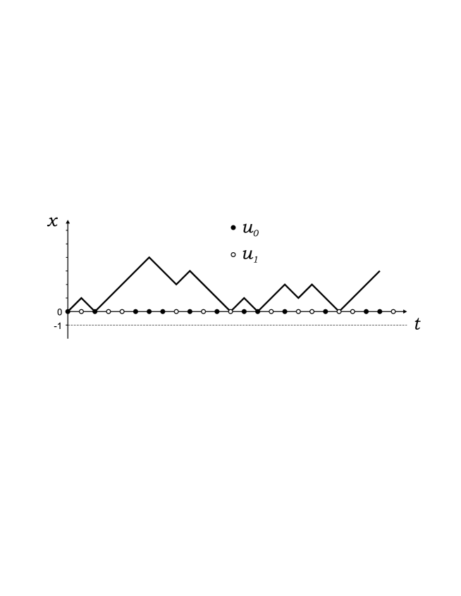
Figure 1: Wetting in a random potential on a line.

To answer the question about the location of the pinning transition find it is more convenient to change distribution of $\beta_{m}$ by changing parameters of $u_{m}$ at fixed temperature $T$ which is conventionally set equal to unity for the rest of the article.

Now we define explicitly what is the pinning (or localization) of the random interface in (1+1)–dimensional wetting problem. Consider the mean–square end-to-end distance, $\left<x^{2}(N)\right>$ of the random interface of length $N$

$$\left<x^{2}(N)\right>=\frac{\displaystyle\sum_{x=0}^{\infty}x^{2}G_{N}(x)}{\displaystyle\sum_{x=0}^{\infty}G_{N}(x)}$$ (2)

There exists some critical value of the energy, $u_{\rm tr}=\ln\beta_{\rm tr}$, which separates two different types of behavior of the mean–square end-to-end distance in the thermodynamic limit:

$$\left<x^{2}(N)\right>\Big{|}_{N\gg 1}=\begin{cases}\Lambda_{1}(u)&\mbox{for $u>u_{\rm tr}$}\\ \Lambda_{2}(u)N&\mbox{for $u<u_{\rm tr}$}\end{cases}$$ (3)

where $\Lambda_{1,2}(u)$ are some positive energy–dependent constants independent of $N$. The value $u_{\rm tr}$ is called the energy of the pinning transition. Formally speaking, for all $u>u_{\rm tr}$ the Eq.(1) has a discrete spectrum, and for $u<u_{\rm tr}$ Eq.(1) has a continuous one. Slightly above the transition point the following critical behavior of the free energy $F_{N}(u)=\ln G_{N}$ of an $N$–step random walk in a half–space $x\geq 0$ is expected:

$$f(u)=\lim_{N\to\infty}\frac{1}{N}F_{N}(u)\equiv\lim_{N\to\infty}\frac{1}{N}\ln G_{N}\Big{|}_{u\to u^{+}_{\rm tr}}={\rm const}\;(u-u_{\rm tr})^{\alpha}$$ (4)

where $\alpha$ is the critical exponent defining the order of the phase transition. In the absence of disorder it was shown no_disorder that $\alpha=2$ which corresponds to an ordinary 2nd order phase transition. In the next subsection we reproduce these calculations. The reason for doing this is to define our notation and introduce important concepts which we shall use in the more complex disordered case.

II.1 Wetting in absence of substrate disorder

We review briefly the situation with no chemical disorder , i.e. when all interaction energies take the same value, $\{u_{m}\}=\{u,u,\ldots,u\}$. Hence, all the Boltzmann weights in Eq.(1) are equal, i.e. $\beta_{m}=\beta$ for $m=1,...N$.

Using the discrete $\sin$–Fourier transform and introducing the generating function, we define the function $G(q,s)$ as follows

$$G(q,s)=\sum_{x=0}^{\infty}\sin qx\sum_{N=0}^{\infty}s^{N}G_{N}(x)$$ (5)

This function satisfies the following integral equation

$$\frac{1}{s}G(q,s)-\frac{\sin q}{s}=\cos q\,G(q,s)+\frac{1}{\pi}(\beta-1)\sin q\int_{0}^{\pi}G(q^{\prime},s)\sin 2q^{\prime}dq^{\prime}.$$ (6)

Introducing

$$A(s)=\int_{0}^{\pi}G(q,s)\sin 2q\,dq$$ (7)

we can rewrite (6) as an algebraic equation for $A(s)$:

$$A(s)=\int_{0}^{\pi}\frac{\sin q\sin 2q}{1-s\cos q}dq+\frac{s}{\pi}(\beta-1)A(s)\int_{0}^{\pi}\frac{\sin q\sin 2q}{1-s\cos q}dq$$ (8)

Solving it we get

$$A(s)=\frac{1}{\displaystyle\left[\int_{0}^{\pi}\frac{\sin q\sin 2q}{1-s\cos q}dq\right]^{-1}-\frac{s}{\pi}(\beta-1)}=\frac{\pi}{s}\,\frac{(1-\sqrt{1-s^{2}})^{2}}{s^{2}-(\beta-1)(1-\sqrt{1-s^{2}})^{2}}$$ (9)

which allows us to write the complete expression for the function $G(q,s)$:

$$G(q,s)=\frac{\sin q}{1-s\cos q}\left(1+\frac{s(\beta-1)}{\pi}A(s)\right)$$ (10)

The inverse Fourier transform applied to (10) gives us

$$G(x,s)=\frac{2}{\pi}\int_{0}^{\pi}G(q,s)\sin qx\,dq=2\left(\frac{1}{s}+\frac{\beta-1}{\pi}A(s)\right)\left(\frac{1-\sqrt{1-s^{2}}}{s}\right)^{x}.$$ (11)

Performing the summation over all $x\geq 0$ we arrive at the following expressions for the functions $G(s)=\sum_{x=0}^{\infty}G(x,s)$ and $\sum_{x=0}^{\infty}x^{2}G(x,s)$:

$$\begin{array}[]{l}\displaystyle G(s)=\sum_{x=0}^{\infty}G(x,s)=2\left(1+\frac{s(\beta-1)}{\pi}A(s)\right)\frac{1}{s-1+\sqrt{1-s^{2}}}\\ \displaystyle\sum_{x=0}^{\infty}x^{2}G(x,s)=\displaystyle 2\left(1+\frac{s(\beta-1)}{\pi}A(s)\right)\frac{(s^{2}+(2+s)(-1+\sqrt{1-s^{2}}))}{(s-1+\sqrt{1-s^{2}})^{3}}\end{array}$$ (12)

The first equation in (12) is the basis for the derivation of the free energy $f=\lim_{N\to\infty}\ln G_{N}$ and we have

$$G_{N}=\frac{1}{2\pi i}\oint G(s)s^{-N-1}\,ds,$$ (13)

while the second equation in (12) provides the mean–square end-to-end distance

$$\left<x^{2}(N)\right>=G_{N}^{-1}\,\frac{1}{2\pi i}\oint\,s^{-N-1}\,ds\sum_{x=0}^{\infty}x^{2}G(x,s).$$ (14)

The integrals in Eqs. (13,14) are performed along a contour in the complex plane of $s$ which lies inside the unit circle. The function $G(s)$ is analytic in the whole complex plane except for the branch cuts on the real axis for $|\textrm{Re}\,s|>1$. In the localized phase the function $G(s)$ has poles for $|s|<1$ on the real axis. In the thermodynamic limit $N\to\infty$ the pinning transition is indicated by appearance of the pole at $s\to s_{\rm tr}=1$, i.e. is determined by the point of divergence of the function $G(s)$ for $s=1$, which, in turn, diverges when the denominator of $A(1)$ tends to zero as $\beta$ approaches the transition point $\beta_{tr}=e^{u_{\textrm{tr}}}$. Thus, we have the following equation for $\beta_{\rm tr}$ (see Eq.(9))

$$s_{\rm tr}-\sqrt{\beta_{\rm tr}-1}\left(1-\sqrt{1-s_{\rm tr}^{2}}\right)\bigg{|}_{s_{\rm tr}=1}=0;\qquad\beta_{\rm tr}\equiv e^{u_{\rm tr}}=2;\qquad u_{\rm tr}=\ln 2\;.$$ (15)

In the localized phase the free energy $f$ in the thermodynamic limit $N\to\infty$ is dominated by the closest to zero pole $s_{0}(\beta)$ of the function $G(s)$ in (12) for some fixed value of $\beta$:

$$s_{0}-\sqrt{\beta-1}\left(1-\sqrt{1-s_{0}^{2}}\right)=0;\qquad s_{0}=\frac{2\sqrt{\beta-1}}{\beta}.$$ (16)

Calculating the contribution of this pole to the integral in Eq. (13), so that:

$$G_{N}=\lim_{N\to\infty}\frac{1}{2\pi i}\oint G(s)s^{-N-1}ds=s_{0}^{-N}=\left(\frac{2\sqrt{\beta-1}}{\beta}\right)^{-N}$$ (17)

we arrive at desired expression of the free energy $f$ in the thermodynamic limit

$$f=-\ln s_{0}=\ln\frac{2\sqrt{\beta-1}}{\beta}.$$ (18)

In the vicinity of the transition point we write $\beta=\beta_{\rm tr}+\delta$, where $\delta\ll\beta_{\rm tr}$. Expanding (18) near $\beta_{\rm tr}=2$, we get

$$f(\beta\to\beta_{\rm tr})=\frac{\delta^{2}}{8}=\frac{(\beta-\beta_{\rm tr})^{2}}{8}=\frac{(u-u_{\rm tr})^{2}}{2}$$ (19)

Comparing (19) to (4) we conclude that $\alpha=2$ and hence the pinning transition on a homogeneous substrate is the standard 2nd order phase transition in accordance with the results no_disorder .

II.2 Wetting in a periodic bimodal potential

Consider now the wetting in a substrate potential with a bimodal periodic distribution of energies $\{u\}=\{u_{0},u_{1},u_{0},u_{1},...,u_{0},u_{1}\}$. We denote by $u_{0}$ and $u_{1}$ the energies belonging to the even/odd time slices correspondingly. This problem has been addressed for the first time in nech_zhang and then considered in much more general setting in subsequent publications swain ; burk ; bauer ; mont . The reason to reconsider this problem is basically methodological: we solve this problem in a matrix form and then in Section II.3 generalize this matrix approach to a substrate with arbitrary period of disorder.

The master equation for the function $G_{N}(x)$ which generalizes (1) is as follows:

$$\left\{\begin{array}[]{l}G_{2N+1}(x)=\frac{1}{2}G_{2N}(x-1)+\frac{1}{2}G_{2N}(x+1)+\frac{1}{2}(\beta_{0}-1)\delta_{x,1}G_{2N}(x+1)\vskip 6.0pt plus 2.0pt minus 2.0pt\\ G_{2N+2}(x)=\frac{1}{2}G_{2N+1}(x-1)+\frac{1}{2}G_{2N+1}(x+1)+\frac{1}{2}(\beta_{1}-1)\delta_{x,1}G_{2N+1}(x+1)\vskip 6.0pt plus 2.0pt minus 2.0pt\\ G_{N}(x=0)=0\vskip 6.0pt plus 2.0pt minus 2.0pt\\ G_{N=0}(x)=\delta_{x,1}\end{array}\right.,$$ (20)

where $\beta_{0,1}=e^{u_{0,1}}$ are the corresponding Boltzmann weights.

Define odd and even functions $G_{N}$:

$$\begin{cases}G_{2N}(x)=W_{N}(x)\vskip 6.0pt plus 2.0pt minus 2.0pt\\ G_{2N+1}(x)=V_{N}(x)\end{cases}$$ (21)

Rewrite (20) in Fourier space using functions $W_{N}(x)$ and $V_{N}(x)$:

$$\left\{\begin{array}[]{l}\displaystyle V_{N}(q)=\cos q\,W_{N}(q)+\frac{\sin q}{\pi}(\beta_{0}-1)\int_{0}^{\pi}W_{N}(q^{\prime})\sin 2q^{\prime}\,dq^{\prime}\vskip 6.0pt plus 2.0pt minus 2.0pt\\ \displaystyle W_{N+1}(q)=\cos q\,V_{N}(q)+\frac{\sin q}{\pi}(\beta_{1}-1)\frac{2}{\pi}\int_{0}^{\pi}V_{N}(q^{\prime})\sin 2q^{\prime}\,dq^{\prime}\vskip 6.0pt plus 2.0pt minus 2.0pt\\ W_{N=0}(q)=\sin q\end{array}\right.$$ (22)

Introducing the generating functions $W(q,s)$ and $V(q,s)$

$$W(q,s)=\sum_{N=0}^{\infty}W(q)s^{N};\qquad V(q,s)=\sum_{N=0}^{\infty}V(q)s^{N}$$ (23)

we can write a closed system of integral equations

$$\left\{\begin{array}[]{l}\displaystyle V(q,s)=\cos q\,W(q,s)+\frac{\beta_{0}-1}{\pi}\sin q\int_{0}^{\pi}W(q^{\prime},s)\sin 2q^{\prime}dq^{\prime}\vskip 6.0pt plus 2.0pt minus 2.0pt\\ \displaystyle W(q,s)=\sin q+s\cos q\,V(q,s)+s\frac{\beta_{1}-1}{\pi}\sin q\int_{0}^{\pi}V(q^{\prime},s)\sin 2q^{\prime}dq^{\prime}\end{array}\right..$$ (24)

It is worth noting that the variable $s$ plays the role of the fugacity of the two-step block and is no longer associated with a single step as, for example, in Eq.(1).

Equations (24) allow for a very convenient matrix formulation which could be later easily generalized to longer periods. Introduce the matrices

$$\hat{A}=\left(\begin{array}[]{cc}0&1\vskip 6.0pt plus 2.0pt minus 2.0pt\\ 1&0\end{array}\right);\quad\hat{B}=\left(\begin{array}[]{cc}\beta_{0}-1&0\vskip 6.0pt plus 2.0pt minus 2.0pt\\ 0&\beta_{1}-1\end{array}\right);\quad\hat{M}_{s}=\left(\begin{array}[]{cc}0&1\vskip 6.0pt plus 2.0pt minus 2.0pt\\ s&0\end{array}\right);\quad\hat{I}=\left(\begin{array}[]{cc}1&0\vskip 6.0pt plus 2.0pt minus 2.0pt\\ 0&1\end{array}\right)$$ (25)

and vectors

$${\bf G}(q,s)=\left(\begin{array}[]{c}V(q,s)\vskip 6.0pt plus 2.0pt minus 2.0pt\\ W(q,s)\end{array}\right);\quad{\bf F}(q)=\left(\begin{array}[]{c}0\vskip 6.0pt plus 2.0pt minus 2.0pt\\ \sin q\end{array}\right)$$ (26)

Rewriting Eq.(24) using (25)–(27), we obtain equation for the vector function ${\bf G}(q,s)$

$${\bf G}(q,s)={\bf F}(q)+\cos q\,\hat{M}_{s}\,{\bf G}(q,s)+\frac{\sin q}{\pi}\hat{B}\hat{M}_{s}\int_{0}^{\pi}\,{\bf G}(q^{\prime},s)\sin 2q^{\prime}\,dq^{\prime}$$ (27)

For further analysis it is convenient to rewrite (27) in the following form

$${\bf G}(q,s)=\left(\hat{I}-\cos q\,\hat{M}_{s}\right)^{-1}{\bf F}(q)+\frac{\sin q}{\pi}\left(\hat{I}-\cos q\,\hat{M}_{s}\right)^{-1}\hat{B}\hat{M}_{s}\int_{0}^{\pi}{\bf G}(q^{\prime},s)\sin 2q^{\prime}\,dq^{\prime}$$ (28)

Define now

$${\bf Q}(s)=\int_{0}^{\pi}{\bf G}(q,s)\sin 2q\,dq$$ (29)

(compare to Eq.(7)). The solution for ${\bf Q}(s)$ reads

$${\bf Q}(s)=\left[\hat{I}-\frac{1}{\pi}\int_{0}^{\pi}dq\,\sin q\sin 2q\,\left(\hat{I}-\cos q\,\hat{M}_{s}\right)^{-1}\hat{B}\hat{M}_{s}\right]^{-1}\int_{0}^{\pi}\left(\hat{I}-\cos q\,\hat{M}_{s}\right)^{-1}{\bf F}(q)\sin 2q\,dq$$ (30)

This equation extends the solution (9) to the periodic bimodal potential $\{u\}=\{u_{0},u_{1},u_{0},u_{1},...,u_{0},u_{1}\}$. Setting parameter $s$ to its critical value $s=s_{\rm tr}=1$ and calculating explicitly the integrals we arrive at the following result

$$\mathbf{Q}(s)=\left(\begin{array}[]{cc}\frac{1}{2-\beta_{1}}&0\\ 0&\frac{1}{2-\beta_{0}}\end{array}\right)\left(\begin{array}[]{c}2\pi\\ 0\end{array}\right)$$ (31)

implying the phase transition at $\beta_{1}=2$. It is clear from the above expression that the value of $\beta_{0}$ is actually irrelevant. This fact reflects the peculiarity of the microscopic model: after an even number of steps the random walk has exactly zero probability to reach $x=2$ from which transition to $x=1$ is controlled by $\beta_{0}$. Mathematically it is reflected in the orthogonality of $\mathbf{F}(q)$ to the eigenvector belonging to the eigenvalue $1/(2-\beta_{0})$ in Eq. (31). We shall see in the next Subsection that this peculiarity persists for arbitrary even periods of the substrate potential.

II.3 Wetting in a potential with arbitrary period length

We can straightforwardly generalize the approach developed in the previous Section to the case of a substrate potential with the period $n$:

$$\{u\}=\{\ldots,\overbrace{u_{0},u_{1},...,u_{n-1}}^{\rm period},...,\overbrace{u_{0},u_{1},...,u_{n-1}}^{\rm period},\ldots\}$$ (32)

i.e. the total substrate consists of $\ell=N/n$ copies of random subchains of length $n$ each. The equations (written already in the Fourier space) which extend (22) to the case of repeating $n$–periodic potential are as follows

$$\left\{\begin{array}[]{l}\displaystyle G_{N}^{(1)}(q)=\cos q\,G_{N}^{(0)}(q)+\frac{\sin q}{\pi}(\beta_{0}-1)\int_{0}^{\pi}G_{N}^{(0)}(q^{\prime})\sin 2q^{\prime}\,dq^{\prime}\vskip 6.0pt plus 2.0pt minus 2.0pt\\ \displaystyle G_{N}^{(2)}(q)=\cos q\,G_{N}^{(1)}(q)+\frac{\sin q}{\pi}(\beta_{1}-1)\int_{0}^{\pi}G_{N}^{(1)}(q^{\prime})\sin 2q^{\prime}\,dq^{\prime}\vskip 6.0pt plus 2.0pt minus 2.0pt\\ ...\vskip 6.0pt plus 2.0pt minus 2.0pt\\ \displaystyle G_{N}^{(n-1)}(q)=\cos q\,G_{N}^{(n-2)}(q)+\frac{\sin q}{\pi}(\beta_{n-2}-1)\int_{0}^{\pi}G_{N}^{(n-2)}(q^{\prime})\sin 2q^{\prime}\,dq^{\prime}\vskip 6.0pt plus 2.0pt minus 2.0pt\\ \displaystyle G_{N+1}^{(0)}(q)=\cos q\,G_{N}^{(n-1)}(q)+\frac{\sin q}{\pi}(\beta_{n-1}-1)\int_{0}^{\pi}G_{N}^{(n-1)}(q^{\prime})\sin 2q^{\prime}\,dq^{\prime}\vskip 6.0pt plus 2.0pt minus 2.0pt\\ \displaystyle G_{N=0}^{(1)}(q)=\sin q\end{array}\right.$$ (33)

As in the case of bimodal disorder rewrite Eqs. (33) in a matrix form

$${\bf G}(q,s)={\bf F}(q)+\cos q\,\hat{M}_{s}\,{\bf G}(q,s)+\frac{\sin q}{\pi}\hat{B}\hat{M}_{s}\int_{0}^{\pi}{\bf G}(q^{\prime},s)\sin 2q^{\prime}\,dq^{\prime}$$ (34)

where

$$\hat{B}=\left(\begin{array}[]{cccccc}\beta_{0}-1&0&0&\dots&0&0\\ 0&\beta_{1}-1&0&&0&0\\ 0&0&\beta_{2}-1&&0&0\\ \vdots&&&\ddots&&\vdots\\ 0&0&0&&\beta_{n-2}-1&0\\ 0&0&0&\dots&0&\beta_{n-1}-1\end{array}\right),\qquad\hat{M}_{s}=\left(\begin{array}[]{cccccc}0&0&\dots&0&0&1\\ 1&0&&0&0&0\\ 0&1&&0&0&0\\ \vdots&&\ddots&&&\vdots\\ 0&0&&1&0&0\\ 0&0&\dots&0&s&0\end{array}\right),$$ (35)

and

$${\bf G}(q,s)=\left(\begin{array}[]{l}G_{1}(q,s)\vskip 6.0pt plus 2.0pt minus 2.0pt\\ \vdots\vskip 6.0pt plus 2.0pt minus 2.0pt\\ G_{n-1}(q,s)\vskip 6.0pt plus 2.0pt minus 2.0pt\\ G_{n}(q,s)\end{array}\right);\quad{\bf F}(q)=\left(\begin{array}[]{c}0\vskip 6.0pt plus 2.0pt minus 2.0pt\\ \vdots\vskip 6.0pt plus 2.0pt minus 2.0pt\\ 0\vskip 6.0pt plus 2.0pt minus 2.0pt\\ \sin q\end{array}\right)$$ (36)

Introducing (as in Eq.(29))

$${\bf Q}(s)=\int_{0}^{\pi}{\bf G}(q,s)\sin 2q\,dq$$ (37)

we get for (34)

$$\mathbf{Q}(s)-\frac{1}{\pi}\int_{0}^{\pi}dq\,\sin q\sin 2q\,\left[\hat{I}-\cos q\,\hat{M}_{s}\right]^{-1}\,\hat{B}\hat{M}_{s}{\bf Q}(s)=\int_{0}^{\pi}dq\,\sin 2q\left[\hat{I}-\cos q\,\hat{M}_{s}\right]^{-1}{\bf F}(q).$$ (38)

where by $\hat{I}$ we have denoted the $N\times N$ unit matrix.

It can be checked that $\hat{B}\hat{M}_{s}=\hat{M}_{s}\hat{B}^{\prime}$, where

$$\hat{B}^{\prime}=\left(\begin{array}[]{cccccc}\beta_{1}-1&0&0&\dots&0&0\\ 0&\beta_{2}-1&0&&0&0\\ 0&0&\beta_{3}-1&&0&0\\ \vdots&&&\ddots&&\vdots\\ 0&0&0&&\beta_{n-1}-1&0\\ 0&0&0&\dots&0&\beta_{n}-1\end{array}\right),\qquad\beta_{n}=\beta_{0}.$$ (39)

Introducing the modified vector ${\bf R}(s)=\hat{B}^{\prime}\,{\bf Q}(s)$ we rewrite Eq. (31) in the following form:

$$\hat{T}_{s}\mathbf{R}(s)=\left[\hat{B^{\prime}}^{-1}-\frac{1}{\pi}\int_{0}^{\pi}dq\,\sin q\sin 2q\,\left[\hat{I}-\cos q\,\hat{M}_{s}\right]^{-1}\,\hat{M}_{s}\right]{\bf R}(s)={\bf C}(s)$$ (40)

with the right hand side

$${\bf C}(s)=\int_{0}^{\pi}dq\,\sin 2q\left[\hat{I}-\cos q\,\hat{M}_{s}\right]^{-1}{\bf F}(q).$$ (41)

The matrix $T_{s}$ in Eq. (40) can be explicitly written as

$$\hat{T}_{s}\equiv\left(\begin{array}[]{cccccc}a_{0}-\dfrac{1}{\beta_{1}-1}&a_{1}&a_{2}&\dots&a_{n-2}&a_{n-1}\\ a_{n-1}&a_{0}-\dfrac{1}{\beta_{2}-1}&a_{1}&&a_{n-3}&a_{n-2}\\ a_{n-2}&a_{n-1}&a_{0}-\dfrac{1}{\beta_{3}-1}&&a_{n-4}&a_{n-3}\\ \vdots&&&\ddots&&\vdots\\ a_{2}&a_{3}&a_{4}&&a_{0}-\dfrac{1}{\beta_{n-1}-1}&a_{1}\\ a_{1}&a_{2}&a_{3}&\dots&a_{n-1}&a_{0}-\dfrac{1}{\beta_{n}-1}\end{array}\right)$$ (42)

and has disorder on its main diagonal only. The nonrandom elements $a_{m}$ are given by the following integrals

$$a_{m}\equiv a_{m}(s)=\frac{1}{\pi}\int_{0}^{\pi}\frac{s\sin q\,\sin 2q\,\cos^{n-m-1}q}{1-s\cos^{n}q}\,dq.$$ (43)

For $n$ even the symmetry of the integrand implies that $a_{m}$ are zero for $m$ odd. The structure of the matrix $T_{s}$ is therefore similar to that of Eq. (31): it does not mix vectors having all but odd/even zero elements. In the following we call these subspaces odd and even sectors. It is important to note that $\mathbf{C}(s)$ belongs to the odd sector and therefore is affected by $\beta_{m}$ with $m$ odd only. For $n$ odd the integrand in the Eq.(43) has no symmetric properties and all elements $a_{m}$ are nonzero. In this case odd and even sectors are mixed by the matrix $T_{s}$ and the physical behavior of the polymer depends on all the values of the disorder potential. The behavior of the coefficients $a_{m}$ is depicted in Fig.2 separately for even and odd total lengths, $n$. In what follows we restrict ourselves to the case of odd values of $n$. This avoids the discussion of the somewhat pathological situation where the pinning transition is insensitive to a macroscopic number of values of the disorder. This situation arises due to the impossibility of return to the origin after an odd number of steps of our random walk and can be eliminated by a different choice of the step probabilities.

Figure 2: Behavior of the coefficients $a_{m}$ for even (a) and odd (b) values of total length $n$.

The pinning transition point in the periodic potential $\beta^{(n)}=\{\beta_{1},...,\beta_{n}\}$ with the period $n$ ($n\gg 1$), where $n$ is assumed to be odd, is determined by the equation

$$\det\hat{T}_{s}\{\beta^{(n)}\}\Big{|}_{s=s_{\rm tr}=1}=0$$ (44)

Let us stress once again that we are in the situation where the sequence $\{\beta\}$ consists of $\ell=N/n$ copies of random subsequences $\{\beta^{(n)}\}$ of length $n$ ($n\gg 1$) each. In Appendix B we show that the pinning transition point in the chain consisting of $\ell$ ($\ell\to\infty$) copies of subsequences $\{\beta^{(n)}\}$ ($n\to\infty$) is the same as in the single subsequence $\{\beta^{(n)}\}$ (i.e. for $\ell=1$) in the limit $n\to\infty$.

III Perturbative calculation of the phase boundary

In this Section we analyze the spectrum of the matrix $\hat{T}\equiv\hat{T}_{s}\Big{|}_{s=s_{\rm tr}=1}$ given by Eq. ((42)) using standard second order perturbation theory. The disorder is supposed to be weak, i.e. the fluctuations of the diagonal elements in Eq. (44) are small compared to their mean value.

III.1 Non-random substrate

We begin with the non-random situation and show that in this case Eqs.(42)–(44) reproduce the results derived in Section II.1. Thus, we shall consider this non-random case as a reference state and develop a perturbation expansion with respect to this unperturbed state. In the absence of any disorder Eq. (44) reduces to

$$\det\hat{T}_{s}(\beta)=\det\left(\begin{array}[]{cccc}a_{0}-(\beta-1)^{-1}&a_{1}&\dots&a_{n-1}\\ a_{n-1}&a_{0}-(\beta-1)^{-1}&\dots&a_{n-2}\\ \vdots&\vdots&\ddots&\vdots\\ a_{1}&a_{2}&\dots&a_{0}-(\beta-1)^{-1}\end{array}\right)=0$$

where the non-random matrix $\hat{T}_{s}(\beta)$ is a special case of a Toeplitz matrix known as a circulant matrix grey . We diagonalize it in the standard way:

$$\hat{T}_{s}=\hat{V}\hat{\Lambda}\hat{V}^{\dagger};\qquad\qquad\hat{V}=\frac{1}{\sqrt{n}}\left\{e^{-2\pi imk/n}\,;\quad m,k=0,1,...,n-1\right\},$$ (45)

where $\hat{\Lambda}$ is the diagonal matrix of the eigenvalues

$$\lambda_{m}=\sum_{k=0}^{n-1}a_{k}e^{-2\pi imk/n}-(\beta-1)^{-1}\qquad m=0,1,...,n-1.$$ (46)

Using the definition (43) for the coefficients $a_{k}$ and by virtue of (46) we have

$$\lambda_{m}(s)=\sum_{k=0}^{n-1}\left[\frac{1}{\pi}\int_{0}^{\pi}\frac{s\sin q\,\sin 2q\,\cos^{n-1-k}q}{1-s\cos^{n}q}\,dq\right]e^{-2\pi imk/n}-(\beta-1)^{-1}.$$ (47)

At the critical value $s=s_{\rm tr}=1$ the last equation becomes

$$\lambda_{m}=2e^{-4\pi im/n}-1-2e^{-4\pi im/n}\sqrt{1-e^{4\pi im/n}}-(\beta-1)^{-1}.$$ (48)

The transition point $\beta_{\rm tr}$ is determined by the condition $\lambda_{0}(\beta_{\rm tr})=0$, yielding the criterion

$$1-(\beta_{\rm tr}-1)^{-1}=0;\qquad\beta_{\rm tr}=2$$ (49)

which reproduces the solution of the non-random problem considered at length in Section II.1.

III.2 Random substrate

Suppose now that the energies $u_{m}=\ln\beta_{m}$ for $m=1,...,n$ are independent random variables distributed according to the law

$$u_{m}=w+\varepsilon\sigma_{m}\qquad\qquad\sigma_{m}=\begin{cases}+1&\mbox{with the probability $\frac{1}{2}$}\\ -1&\mbox{with the probability $\frac{1}{2}$}\end{cases}$$ (50)

and find eigenvalues and eigenvectors of the perturbed matrix $T$ in the second order of series expansion in the strength of the disorder. Expanding the diagonal elements of the matrix $\hat{T}$ (Eq.(42)) in $\varepsilon\ll 1$, we get

$$Q_{i}=a_{0}-(e^{u_{i}}-1)^{-1}=a_{0}-\left(e^{w+\sigma_{i}\varepsilon}-1\right)^{-1};\qquad(i=1,2,...,n)$$ (51)

Expanding (51), we arrive finally at the following expression for the diagonal elements $Q_{i}$ of the matrix $\hat{T}$

$$Q_{i}=a_{0}-(e^{w}-1)-p_{0}+p_{1}\sigma_{i}$$ (52)

where

$$\begin{cases}\displaystyle p_{0}=\frac{1}{2}\frac{e^{w}(e^{w}+1)}{(e^{w}-1)^{3}}\,\varepsilon^{2}\vskip 6.0pt plus 2.0pt minus 2.0pt\\ \displaystyle p_{1}=\frac{e^{w}}{(e^{w}-1)^{2}}\,\varepsilon\end{cases}$$ (53)

The matrix $\hat{T}_{s}\{\beta^{(n)}\}$ up to the second order perturbation on $\varepsilon$ reads

$$\hat{T}_{s}\{\beta^{(n)}\}=\hat{A}+\hat{B}=\hat{T}_{s}(e^{w})-p_{0}\hat{I}+\left(\begin{array}[]{cccc}p_{1}\sigma_{1}&0&\dots&0\\ 0&p_{1}\sigma_{2}&&0\\ \vdots&&\ddots&\vdots\\ 0&0&\dots&p_{1}\sigma_{n}\end{array}\right)$$ (54)

where the matrices $\hat{A}=\hat{T}_{s}(e^{w})-p_{0}\hat{I}$ and $\hat{B}$ are correspondingly the unperturbed and perturbed parts of the matrix $T$ (by $\hat{I}$ we have denoted the unit $n\times n$ matrix).

Standard 2nd order perturbation theory leads to the following expression for the perturbed eigenvalue $\lambda_{m}^{\prime}$:

$$\lambda_{m}^{\prime}\{\beta^{(n)}\}=\lambda_{m}+{\bf v}_{m}\hat{B}\;{\bf v}^{\top}_{m}+\sum_{m^{\prime}\neq m,\nu}\frac{\left|{\bf v}^{(\nu)}_{m}\hat{B}\;{\bf v}^{\top,(\nu)}_{m^{\prime}}\right|^{2}}{\lambda_{m}-\lambda_{m^{\prime}}}$$ (55)

where $\nu$ is the degeneracy of the eigenvalues and the eigenvectors ${\bf v}_{m}$ are the columns of the matrix (45). In what follows we are interested in the computation of the largest eigenvalue $\lambda_{0}^{\prime}$.

For any particular sequence $\{\beta^{(n)}\}$ the transition point is determined by the condition

$$0=\lambda^{\prime}_{0}\{\beta^{(n)}\}=1-\frac{1}{e^{w}-1}-p_{0}+\frac{p_{1}}{n}\left(\sum_{k=0}^{n-1}\sigma_{k}\right)+\frac{p_{1}^{2}}{n^{2}}\left(\sum_{m^{\prime}\neq 0}\frac{1}{\lambda_{0}-\lambda_{m^{\prime}}}\sum_{k=0}^{n-1}\sum_{k=0}^{n-1}\sigma_{k}\sigma_{k^{\prime}}e^{-2\pi m^{\prime}(k-k^{\prime})/n}\right)$$ (56)

Let us denote

$$\left\{\begin{array}[]{l}\displaystyle S_{1}=\sum_{k=0}^{n-1}\sigma_{k}\\ \displaystyle S_{2}=\sum_{m^{\prime}\neq 0}\frac{1}{\lambda_{0}-\lambda_{m^{\prime}}}\sum_{k=0}^{n-1}\sum_{k=0}^{n-1}\sigma_{k}\sigma_{k^{\prime}}e^{-2\pi m^{\prime}(k-k^{\prime})/n}\end{array}\right.$$ (57)

and expand the coefficients $p_{0}$ and $p_{1}$ for small $w$ in the vicinity of $\ln 2$ up to the 2nd order in $w$ and $\varepsilon$:

$$\begin{array}[]{l}\displaystyle p_{0}=3\varepsilon^{2}+13\varepsilon^{2}(\ln 2-w)+\frac{75}{2}\varepsilon^{2}(\ln 2-w)^{2}\vskip 6.0pt plus 2.0pt minus 2.0pt\\ \displaystyle p_{1}=2\varepsilon+6\varepsilon(\ln 2-w)+13\varepsilon(\ln 2-w)^{2}\end{array}$$ (58)

In the 2nd order perturbation series we keep only the terms up to the second order in $\tilde{w}=\ln 2-w$ and $\varepsilon$:

$$\lambda^{\prime}_{0}=-2\tilde{w}-3{\tilde{w}}^{2}-3\varepsilon^{2}+(2\varepsilon+6\varepsilon\tilde{w})\frac{S_{1}}{n}+4\varepsilon^{2}\frac{S_{2}}{n^{2}}=0$$ (59)

Solving the quadratic equation $\tilde{w}(\varepsilon)=0$ (we have chosen the branch, on which $w\to\ln 2$ as $\varepsilon\to 0$) and re-expanding the final expression in $\varepsilon$ up to the 2nd order, we get

$$\tilde{w}=-\varepsilon\frac{S_{1}}{n}+\frac{1}{2}\varepsilon^{2}\left(3\frac{S_{1}^{2}}{n^{2}}+4\frac{S_{2}}{n^{2}}-3\right)$$ (60)

Let us stress that the expression (60) is valid for any distribution ${\cal P}\{\sigma\}$ of random Ising–type variable $\sigma_{i}$. The general form of the transition curve in the 2nd order approximation reads

$$\tilde{w}=-\varepsilon\frac{\left<S_{1}\right>}{n}+\frac{1}{2}\varepsilon^{2}\left(3\frac{\left<S_{1}^{2}\right>}{n^{2}}+4\frac{\left<S_{2}\right>}{n^{2}}-3\right)$$ (61)

The terms proportional to $\left<S_{1}\right>$ vanish due to the symmetry $\sigma_{i}\leftrightarrow-\sigma_{i}$. The calculation of the second order correction is straightforward though rather tedious and is given in Appendix A. The final result for the averaged transition point $w$ in the limit of large $n$ reads

$$\tilde{w}=\frac{\varepsilon^{2}}{2}$$ (62)

so that the phase diagram is determined by the equation

$$w=\ln 2-\frac{\varepsilon^{2}}{2}$$ (63)

This result of the perturbation theory for the phase boundary $w(\varepsilon)$ is shown in Fig.3 by dashed line. For $\varepsilon<0.5$ there is a good agreement of the perturbative approach with the numerical data and results of our renormalization group computations of the next Section.

IV Simple RG consideration

The location of the localization (wetting) transition can be found following a simple renormalization argument. We start with the master equation (3) in the Fourier space

$$G_{N+1}(q)=\cos q\,G_{N}(q)+\big{(}\beta_{N}-1\big{)}\frac{\sin q}{\pi}\int_{0}^{\pi}\!dq^{\prime}\,\sin 2q^{\prime}\,G_{N}(q^{\prime})$$ (64)

and iterate it twice

$$G_{N+2}(q) = \cos^{2}q\,G_{N}(q)$$ (65)

$$+ \big{(}\beta_{N}-1\big{)}\frac{\sin q\cos q}{\pi}\int_{0}^{\pi}\!dq^{\prime}\,\sin 2q^{\prime}\,G_{N}(q^{\prime})+\big{(}\beta_{N+1}-1\big{)}\frac{\sin q}{\pi}\int_{0}^{\pi}\!dq^{\prime}\,\sin 2q^{\prime}\cos q^{\prime}\,G_{N}(q^{\prime})$$ (66)

$$+ \big{(}\beta_{N}-1\big{)}\big{(}\beta_{N+1}-1\big{)}\frac{\sin q}{\pi^{2}}\int_{0}^{\pi}\!dq^{\prime}\,\sin 2q^{\prime}\sin q^{\prime}\int_{0}^{\pi}\!dq^{\prime\prime}\,G_{N}(q^{\prime\prime}).$$ (67)

The last term in the r.h.s. vanishes due to the orthogonality. The second and third term describe processes of two–step arrival to $x=1$. We note that in the long–wavelength limit $q\to 0$ they are identical as seen by replacing the cosines by unity. This corresponds to neglecting variation in $G_{N}(x)$ on scale of the lattice spacing and will be justified later. Combining these terms we obtain an expression similar to the small $q$ version of Eq.(64) with modified random part

$$G_{N+2}(q)-G_{N}(q)=-q^{2}G_{N}(q)+\big{(}\beta_{N}+\beta_{N+1}-2\big{)}\frac{\sin q}{\pi}\int_{0}^{\pi}\!dq^{\prime}\,\sin 2q^{\prime}G_{N}(q^{\prime})$$ (68)

and corresponding to the double time interval. By this procedure the random potential has been normalized to the arithmetic mean of two subsequent terms:

$$\beta^{\prime}_{N/2}=\frac{\beta_{N}+\beta_{N+1}}{2}$$ (69)

The probability distribution of the renormalized disorder $\beta^{\prime}$ is related to that of $\beta$ as follows. Let $P(\beta)$ be a probability distribution of $\beta_{j}$ and $P^{\prime}(\beta^{\prime})$ the one of the new variables. The corresponding Fourier transforms (characteristic functions) $\xi(\lambda)$ and $\xi^{\prime}(\lambda^{\prime})$ are related as

$$\xi^{\prime}(\lambda^{\prime})=\xi^{2}(\lambda^{\prime}/2).$$ (70)

The fixed point of this transformation is the exponential function

$$\xi^{\prime}(\lambda)=\xi(\lambda)=\exp(i\lambda\left<\beta\right>)$$ (71)

which is just a consequence of the Central Limit Theorem.

Therefore the disorder $\beta_{j}=e^{u_{j}}$ can be just replaced by their mean value $\left<\beta_{j}\right>=\left<e^{u_{j}}\right>$ in the long–wavelength limit. The crucial observation is that $\left<e^{u_{j}}\right>\neq e^{-\left<u\right>}$, so fluctuations of $u_{j}$ modify the localization criterion. For disorder discussed in the previous section (see (50)). The mean value of $\beta_{j}$ is given by

$$\left<\beta_{j}\right>=e^{w}\cosh\varepsilon$$ (72)

so it depends on both parameters, the mean value, $w$, and fluctuations, $\varepsilon$. The localization criterion reads from (17)

$$\bar{\beta}=e^{w}\cosh\epsilon=2\qquad\Rightarrow\qquad w=\ln 2-\ln\cosh\varepsilon$$ (73)

The lowest order in expansion of this expression in powers of $\varepsilon$ yields the result of the perturbation theory (63). The graphical representation of the RG phase boundary (73) is shown in Fig.3 by solid line.

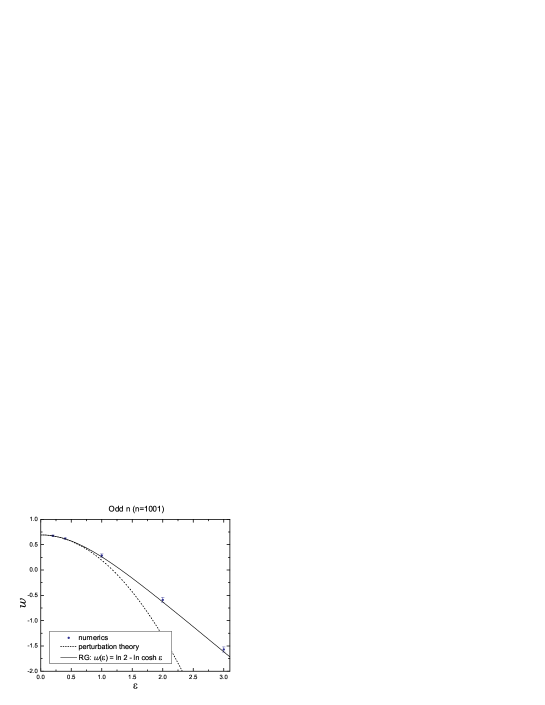
Figure 3: Phase diagram for quenched disorder in the plane $(\varepsilon,w)$. The renormalization group computations and perturbation theory are depicted by solid and dashed lines correspondingly. The results of numerical averaging are shown for odd $n$ ($n=1001$).

Finally, we observe that from the expressions (9)–(10) it follows that the bound state contribution to the Fourier transform

$$G_{N}(q)\sim\frac{\beta-2}{2\beta}\frac{\sin q}{1-s_{0}\cos q}s_{0}^{-N},\qquad\qquad s_{0}=\frac{2\sqrt{\beta-1}}{\beta}$$ (74)

is strongly peaked around $q=0$ close to the transition point $\beta=2$. This justifies replacing $\cos q$ by unity in the integrals in Eq.(65).

V Numerical analysis of the depinning transition

To visualize the eigenvalues of the matrix $\hat{T}$ , consider the case of absence of any disorder, i.e. take in Eq.(42) the homogeneous sequence $\{\beta^{(n)}\}$ with $\beta_{j}\equiv\beta$ for all $j=1,...,n$. In Fig.4 we have plotted the eigenvalues $\lambda_{m}$ ($m=1,...,n$) of the matrix $\hat{T}$ in the complex plane for two values $w=\ln 2.1$ and $w=\ln 2.0$ (transition point) for even (a) and odd (b) values of $n$. For even values of $n$ the spectrum of the pure matrix $\hat{T}$ is doubly degenerate, while for odd $n$ this degeneracy disappears. In what follows we consider odd $n$ only.

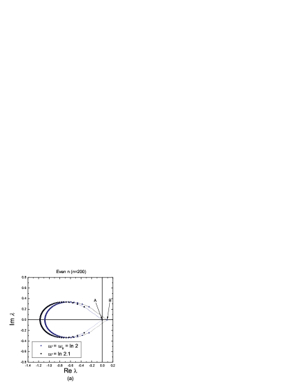
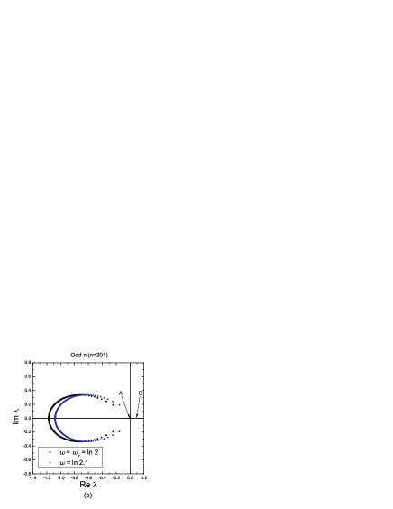
Figure 4: The eigenvalues $\lambda_{m}$ of the matrix $\hat{T}$ in the complex plane $({\rm Re}\lambda,{\rm Im}\lambda)$ for: (a) even $n$ ($n=200$) and (b) odd $n$ ($n=201$) for two different values of $w$: $w=\ln 2.0$ (transition point) and $w=\ln 2.1$.

We now consider disorder generated by the distribution (50) and find numerically the location of the pinning transition. The general procedure is very simple: we fix some value $\varepsilon$, then generate ensemble of random sequences $\beta^{(n)}$ from the distribution (50) and find for each sequence such a $w$ at which the real eigenvalue of the matrix $\hat{T}$ crosses zero implying the condition

$$\lim_{n\to\infty}\det\hat{T}\{\beta_{1},...,\beta_{n}\}=0$$ (75)

The obtained critical value is then averaged over realizations $\{\beta^{(n)}\}$ of quenched disorder. We take the size of the $n\times n$ matrix $\hat{T}$ equal to $n=1001$. In Fig.3 we show the points corresponding to the averaged phase boundary for the ensemble of quenched sequences $\{\beta^{(n)}\}$ in the space of the parameters $\varepsilon,w$.

Figure 5: Sample plots of the location of eigenvalues of the matrix $\hat{T}$ for $\varepsilon=1.0$ and different values of $w$ ($n=1001$).

In the next section we discuss the obtained numerical phase diagram.

VI Conclusions

In this paper we have discussed the problem of wetting of a one–dimensional random walk on a half–line $x\geq 0$ in a short–ranged periodic potential located at the origin $x=0$. When the period of the potential becomes equal to the length of the random walk trajectory, then one could conjecture that the trajectory under consideration is interacting with the quenched random potential. In other words, we approach the random potential, increasing more and more the period of the substrate potential.

The most attention is paid to the question concerning the location of the transition point averaged over all equally weighted realizations of the disorder. We have shown that for any specific disorder realization, the transition point can be obtained from the condition that the determinant of the matrix (42) (with the entries (43)) is equal to zero at $s=1$ — see Eq.(44). The period of the substrate is given the size $n$ of the matrix (42) which remains to be very large but finite in our consideration, and the fugacity $s$ is conjugate to the number of copies, $\ell=N/n$, of $n$–periodic potential (so, $N$ is the total length of the substrate). Setting the fugacity $s$ in (42)–(43) to its limiting value $s_{\rm tr}\equiv 1$ amounts to the consideration of $\ell\to\infty$ copies of the system.

One may worry that in the thermodynamic limit the transition point in the periodic sequence of $\ell$ ($\ell\to\infty$) subchains each of length $n$ ($n\gg 1$) differs from the transition point in a single ($\ell=1$) subchain (of the same primary structure) of length $n$ ($n\to\infty$). However this is not true and in Appendix B we show that the transition point is not sensitive to the sequence of thermodynamic limits and for $n\to\infty$ is independent on number of copies, $\ell$.

We have compared the results of our numerical simulations performed in a wide range of disorder strengths with the results of the perturbation theory for weak disorder, and the results of a simple renormalization group consideration. The results obtained allow us to conclude that for weak disorder $\varepsilon<0.5$ all approaches (including the perturbation theory) are in a good agreement. For sufficiently high disorder strengths $\varepsilon>\varepsilon_{\rm pert}\sim 0.5$ the second order perturbation theory fails, while the results of the renormalization group always agree with the numerical simulations — see the Fig.3. This point deserves some special discussion. Namely, recall that results of the RG computations claim the existence of the averaged Boltzmann weight which governs the behavior of the system under renormalization. This fact signals the existence of an effective preaveraged (with respect to the disorder) annealed system with averaged Boltzmann weight $\left<e^{u_{m}}\right>$. This statement is consistent with the conclusion of works forgacs ; gro , but contradicts the statement that the disorder is marginally relevant formulated for the first time in derrida .

Let us note at the very end that the advantage of our matrix approach is its transparency. We have made no any uncontrolled assumption and have reduced very complicated initial problem with many degrees of freedom to the well posed problem of finding eigenvalues of some random matrix with a relatively simple structure. The localization criteria $\det T\{\beta_{1},...,\beta_{N}\}=0$ for a random sequence $\{\beta_{1},...,\beta_{N}\}$ in the limit $N\to\infty$ is exact for any strengths and any distributions of $\beta_{i}$ ($i=1,...,N$).

The results obtained in our work allow us to state that even for strong disorder the shift of the averaged pinning point of the random walk in the ensemble of random realizations of substrate disorder is indistinguishable from the pinning point of the system with preaveraged (i.e. annealed) Boltzmann weight.

Appendix A Perturbation theory for matrix $T_{s}$

The terms in Eq. (61) are

$$\left\{\begin{array}[]{l}\displaystyle\frac{1}{n}\left<S_{1}\right>=\frac{1}{n}\sum_{k=0}^{n-1}\left<\sigma_{k}\right>\\ \displaystyle\frac{1}{n^{2}}\left<S_{1}^{2}\right>=\frac{1}{n^{2}}\sum_{k=0}^{n-1}\sum_{k^{\prime}=0}^{n-1}\left<\sigma_{k}\sigma_{k^{\prime}}\right>\\ \displaystyle\frac{1}{n^{2}}\left<S_{2}\right>=\frac{1}{n^{2}}\sum_{m^{\prime}\neq 0}\frac{1}{\lambda_{0}-\lambda_{m^{\prime}}}\sum_{k=0}^{n-1}\sum_{k=0}^{n-1}\left<\sigma_{k}\sigma_{k^{\prime}}\right>e^{-2\pi m^{\prime}(k-k^{\prime})/n}\end{array}\right.$$ (76)

The computation of $\left<S_{1}\right>$ and $\left<S_{1}^{2}\right>$ where averaging $\left<...\right>$ is performed over the symmetric distribution ${\cal P}\{\sigma\}$, is straightforward:

$$\frac{1}{n}\left<S_{1}\right>=0;\quad\frac{1}{n^{2}}\left<S_{1}^{2}\right>=\frac{1}{n}$$ (77)

Using (48), we obtain for the unperturbed part $\hat{A}$ of the matrix $\hat{T}$ (Eq.(54)) the following expression for the eigenvalues

$$\lambda_{m}=2e^{-4\pi im/n}-1-2e^{-4\pi im/n}\sqrt{1-e^{4\pi im/n}}-(e^{w}-1)^{-1}-p_{0}$$ (78)

Taking into account that

$$\sqrt{1-e^{4\pi im/n}}=\sqrt{2\sin\frac{2\pi m}{n}}\;e^{i\pi(m/n-1/4)},$$

we can substitute (78) into last line of (76). Thus we get

$$\frac{1}{n^{2}}\left<S_{2}\right>=\frac{1}{n}\sum_{m^{\prime}\neq 0}\frac{1}{\lambda_{0}-\lambda_{m^{\prime}}}=\frac{1}{n}\sum_{m^{\prime}\neq 0}^{n-1}\left(2-2e^{-4\pi im^{\prime}/n}+2e^{-\pi i(1/4+3m^{\prime}/n)}\sqrt{2\sin\frac{2\pi m^{\prime}}{n}}\right)^{-1}$$ (79)

Since the eigenvalues are distributed symmetrically with respect to the real axis (see Fig.4a), the sum $\sum_{m}\frac{1}{\lambda_{0}-\lambda_{m^{\prime}}}$ takes only the real values. After some algebra, we arrive at the final equation for the expectation $\left<S_{2}\right>$:

$$\frac{1}{n^{2}}\left<S_{2}\right>=\frac{2}{n}\sum_{m^{\prime}\neq 0}^{(n-1)/2}\;\frac{1-\cos\frac{4\pi m^{\prime}}{n}+\sqrt{2\sin\frac{2\pi m^{\prime}}{n}}\cos\left(\frac{3\pi m^{\prime}}{n}+\frac{\pi}{4}\right)}{\sin\frac{2\pi m^{\prime}}{n}\left(1-2\sqrt{2\sin\frac{2\pi m^{\prime}}{n}}\sin\left(\frac{3\pi m^{\prime}}{n}+\frac{\pi}{4}\right)+2\sin\frac{2\pi m^{\prime}}{n}\right)}$$ (80)

In the limit $n\to\infty$ the sum in (80) can be replaced by the integral:

$$\frac{1}{n^{2}}\left<S_{2}\right>\approx 2\int_{0}^{1/2}\frac{1-\cos 4\pi x+\sqrt{2\sin 2\pi x}\cos\left(3\pi x+\frac{\pi}{4}\right)}{\sin 2\pi x\left(1-2\sqrt{2\sin 2\pi x}\sin\left(3\pi x+\frac{\pi}{4}\right)+2\sin 2\pi x\right)}dx=1$$ (81)

Substituting (77) and (81) into (61) we arrive in the limit $n\to\infty$ at the desired equation (62).

Appendix B Independence of phase boundary on number of periods $\ell$ in the thermodynamic limit

It follows from the general definition of the generating functions, that in order to consider the phase transition in an individual period of the substrate potential (32), i.e. for $\ell=1$, we should shift the fugacity $s$ (conjugated to $\ell$) away from its marginal value $s=s_{\rm tr}=1$ (corresponding to $\ell\to\infty$) to some value $s_{\ell}$ lying in the interval $0<s_{\ell}<s_{\rm tr}$.

The number of periods, $\ell$, is controlled by the fugacity $s_{\ell}$. So, to compare the transition points in chains of different periods, we should normalize the Boltzmann weights of chain of $\ell$ periods per a weight of a a single period, $s_{\ell}$ (for $\ell=1$). Dividing the Boltzmann weights in the matrix $T_{s}$ (see Eq.(42)) by $s_{\ell}$, we get: $(\beta-1)\to(\beta^{*}-1)/s_{\ell}$. Now we could investigate how the normalized transition point, $\beta^{*}_{\rm tr}$, depends on the typical fugacity $s_{\ell}$. It is easy to see that in the absence of any disorder (i.e. for $\varepsilon=0$) the eigenvalue $\lambda_{0}$ (see Eq.(47) for $m=0$) is given by the following integral

$$\lambda_{0}(s_{\ell})=\frac{s_{\ell}}{\pi}\int_{0}^{\pi}\frac{\sin q\,\sin 2q\,(1-\cos^{n}q)}{(1-s_{\ell}\,\cos^{n}q)(1-\cos q)}\,dq-\frac{s_{\ell}}{\beta^{*}-1}$$ (82)

The equation $\lambda_{0}(s_{\ell})=0$ in the limit $n\to\infty$ determines the position of the normalised transition point, $\beta^{*}_{\rm tr}(s_{\ell})$. One can easily verify that in the limit $n\to\infty$ the integral (82) is independent of $s_{\ell}$ and, hence, $\beta^{*}_{\rm tr}(s_{\ell})=2$ for any $0<s_{\ell}<s_{\rm tr}$. The same conclusion holds for $\varepsilon\neq 0$ in the matrix $T_{s}$: the transition point in the limit $n\to\infty$ for any random primary sequence is independent of the effective fugacity $s_{\ell}$ corresponding to finite number of periods, $\ell$.

So, we conclude that in the thermodynamic limit the transition point in the periodic sequence of $\ell$ ($\ell\to\infty$) random subchains each of length $n$ ($n\gg 1$) coincides with the transition point in a single ($\ell=1$) random subchain (of the same primary structure) of length $n$ ($n\to\infty$).

This conclusion has very transparent physical sense. Namely, consider from the very beginning the random walk with periodic boundary conditions in the space. The simplest way is to suppose that the first ($t=0$) and last ($t=N$) steps of the random trajectory are always attached to the random substrate at the point $x=0$. For such a periodic system the location of the transition point is exactly given by the equation

$$\lim_{N\to\infty}\det T\{\beta_{1},\beta_{2},...,\beta_{N}\}=0$$

Hence, the transition point is not sensitive to whether the terminal step of the random walk is attached to the surface or not. This is evident in the localized regime where the fluctuations of mean–square end-to-end distance are constant (see Eq.(3)).

References

• (1) D.B. Abraham, Phys. Rev. Lett. 44, 1165 (1980); and in Phase Transitions and Critical Phenomena, edited by C. Domb and J.L. Lebowitz (Academic Press, London, 1986), Vol. 10
• (2) G. Forgacs, J.L. Luck, T.M. Nieuwenhuizen, H. Orland, Phys. Rev. Lett. 57, 2184 (1986); J. Stat. Phys. 51, 29 (1988); G. Forgacs, R. Lipowsky, T.M. Nieuwenhuizen, in Phase Transitions and Critical Phenomena, edited by C. Domb and J.L. Lebowitz (Academic Press, London, 1991), Vol. 14
• (3) A.Yu. Grosberg, E.I. Shakhnovich, Sov. Phys. JETP 64, 493; ibid 1284
• (4) B. Derrida, V. Hakim, J. Vannimenus, J. Stat. Phys. 66, 1189 (1992)
• (5) S. Stepanow, A.L. Chudnovskiy, J. Phys. A: Math. Gen. 35, 4229 (2002)
• (6) L.H. Tang, H. Chaté, Phys. Rev. Lett. 86, 830 (2001)
• (7) K. Alexander, ArXiv: math.PR/0610008
• (8) F.L. Toninelli, ArXiv: math-ph/0701063
• (9) G. Giacomin, F.L. Toninelli, Phys. Rev. Lett. 96 070602 (2006); G. Giacomin, F.L. Toninelli, Commun. Math. Phys. 266 1 (2006)
• (10) A. Naidenov, S. Nechaev, J. Phys. A: Math. Gen. 34, 5625 (2001)
• (11) T.W. Burkhardt, J. Phys. A: Math. Gen. 14, L63 (1981); J.T. Chalker, J. Phys. A: Math. Gen. 14, 2431 (1981); S.T. Chui and J.D. Weeks Phys. Rev. B 23, 2438 (1981); J.M.J. van Leeuwen and H.J. Hilhorst, Physica 107A 319 (1981).
• (12) S. Nechaev, Y.C. Zhang, Phys. Rev. Lett. 74, 1815 (1995)
• (13) P.S Swain, A.O. Parry, J. Phys. A: Math. Gen, 30, 4597 (1997)
• (14) T.W. Burkhardt, J. Phys. A: Math. Gen, 31, L549 (1998)
• (15) C. Bauer, S. Dietrich, Phys. Rev. E 60, 6919 (1999)
• (16) C. Monthus, T. Garel, H. Orland, Eur. Phys. J. B 17, 121 (2000)
• (17) R.M. Gray, Toeplitz and Circulant Matrices: A Review, in Foundations and Trends in Communications and Information Theory 2, 155 (2006)