$uvby-H_{\beta}$ CCD photometry and membership segregation of the open cluster NGC 2682 (M 67).

Following deep astrometric and photometric study of the cluster NGC 2682 (M 67), we are able to accurately determine its fundamental parameters. Being an old and rich cluster, M 67 is a relevant object for the analysis of the Galactic disk evolution. M 67 is well studied but the lack of a wide and deep Strömgren photometric study makes our results worthwhile. The brightest stars of the open cluster M 67 were used as $uvby-H_{\beta}$ standard stars in our studies of NGC 1817 and NGC 2548, and the extension of the field covered, as well as the amount of observations, allowed to obtain the best set of Strömgren data ever published for this cluster. We discuss the results of our CCD $uvby-H_{\beta}$ intermediate-band photometry, covering an area of about 50$\arcmin\times$50$\arcmin$ down to $V\sim$ 19. Moreover, a complete membership segregation based on astrometric and photometric criteria is obtained. The photometric analysis of a selected sample of stars yields a reddening value of $E(b-y)$ = 0.03$\pm$0.03, a distance modulus of $V_{0}-M_{V}$ = 9.7$\pm$0.2 and [Fe/H] = 0.01$\pm$0.14. Through isochrone fitting we found an age of $\log t$ = 9.6$\pm$0.1 (4.2$\pm$0.2 Gyr). A clump of approximately 60 stars around $V$ = 16, $(b-y)$ = 0.4 could be interpreted as a population of pre-cataclysmic variable stars (if members), or as a stream of field G-type stars placed at twice the distance of the cluster (if non-members).

1 Introduction

NGC 2682 (C0847+120), also known as M 67, in Cancer [$\alpha_{2000}$=8${}^{\mathrm{h}}51^{\mathrm{m}}\hbox to0.0pt{\hss.}3$, $\delta_{2000}=+11{\degr}50\arcmin$; $l\leavevmode\nobreak\ =215^{\circ}\hbox to0.0pt{\hss.}66$, $b\leavevmode\nobreak\ =+31^{\circ}\hbox to0.0pt{\hss.}91$] is probably the most thoroughly studied old open cluster in the Galaxy, thanks to its small distance from us (estimated to be $\sim$ 900 pc). Typically quoted values for the age of the cluster ($\sim$ 4 Gyr) place it among the oldest open clusters. In our astrometric and photometric study of several open clusters (Balaguer-Núñez et al., 2004a; Balaguer-Núñez et al., 2005), the photometric standard stars were taken from this cluster (Nissen et al., 1987), thus high-quality Strömgren wide-field CCD photometry of it also resulted from our observations. The existence of a proper motions study (Zhao et al., 1993) of similar quality and characteristics of those used in our study of other clusters (based on the same plate material and methods, by the Shanghai Astronomical Observatory), allowed us to apply the same techniques and analysis tools to this cluster. This paper on M 67 closes the series at this stage of our open cluster programme.

Photometric studies of M 67 have been performed by several authors. Montgomery et al. (1993) have presented a deep ($V\sim$ 20) $UBVI$ CCD photometry of 1468 stars within 15$\arcmin$ of the centre of the cluster, and Fan et al. (1996) have studied spectrophotometry of similar depth in nine BATC intermediate-band filters for stars in a 1$\aas@@fstack{\circ}$92 $\times$ 1$\aas@@fstack{\circ}$92 area centred on the cluster. In addition, variability studies have been performed in this cluster, most notably by Gilliland et al. (1993), who conducted a very sensitive, highly temporally sampled study of stars in the central few arcmin of the cluster. Stassun et al. (2002) using differential CCD photometry to search for variability, obtained sensitive photometry of 990 stars in a roughly square region one-third of a degree on a side centred 5$\arcmin$ north of the cluster centre. Sandquist (2004) also as a by-product of variability studies, conducted a high precision $VI$ colour-magnitude diagram analysis.

Nissen et al. (1987) obtained accurate $uvby-H_{\beta}$ photoelectric photometry of a sample of 79 stars within a radius of 10$\arcmin$ from the centre, from the subgiant branch down to the unevolved main sequence. For this reason stars in M 67 were used by us as photometric standard stars for the observations of NGC 1817 and NGC 2548 (Balaguer-Núñez et al., 2004a; Balaguer-Núñez et al., 2005). The amount of observations taken in our programme allowed us to obtain high quality photometry of this cluster. In spite of being a well studied cluster, our Strömgren photometry deserves an analysis due both to its deepness and to the extension of the covered area.

There are also a number of proper motion and radial velocity studies. Sanders (1977) calculated probabilities of membership based on relative proper motions of 1866 stars in the cluster field with a limiting photographic magnitude of $\sim$17. From 10 plate pairs of different origin and with a maximum epoch difference of 68 years, he found 649 probable members. Girard et al. (1989) gave relative proper motions for 663 stars in an area of 42$\arcmin\times$34$\arcmin$ from 44 plates with a maximum separation of 66 years. Although the plates used were of different depths, the deepest plates provided a limiting visual magnitude down to 16. In 1993, Zhao et al. derived relative proper motions for 1046 stars within a 1$\aas@@fstack{\circ}$5 $\times$ 1$\aas@@fstack{\circ}$5 area in the region from PDS measurements of 9 plates with a maximum epoch difference of 80 years and a magnitude limit $V\sim$ 15.5.

On the other hand, the radial velocity studies by Mathieu et al. (1986, 1990) gave precise radial-velocity measurements for 170 stars, including all main-sequence stars brighter than $V$ = 12.8.

In this paper we discuss the results of our CCD photometric study, covering an area of about 50$\arcmin$$\times$50$\arcmin$ (Fig. 1) down to $V$$\sim$ 19. Section 2 contains the details of the CCD observations and their reduction and transformation to the standard system. In Sect. 3 we discuss a new membership segregation based on the combination of parametric and non-parametric methods applied to the above-mentioned proper motions from Zhao et al. (1993). This study was selected among all other existent because it covers the biggest area and largest epoch difference. Also, this material is fully homogeneous with that used by us for the other clusters in this series, as from the point of view of telescope and plates, as from the point of view of proper motion treatment and reduction. This section includes a discussion on the limits on proper motions detection of binarity.

In Sect. 4 we discuss the colour-magnitude diagram and identify the sample of probable cluster members using astrometric as well as photometric criteria. Section 5 contains the derivation of the fundamental cluster parameters of reddening, distance, metallicity and age. Section 6 studies the multiple star systems, blue stragglers and a new feature on the colour-magnitude diagram. Section 7 summarizes our conclusions.

2 The Data

2.1 Observations

The Strömgren CCD photometry of the area was obtained at Calar Alto Observatory (Almería, Spain) in January 2000 using the 1.23 m telescope of Centro Astronómico Hispano-Alemán (CAHA). Further data were obtained at Observatorio del Roque de los Muchachos (ORM, La Palma, Canary Islands, Spain) in February 2000 using the 2.5 m Isaac Newton Telescope (INT) of ING (equipped with the Wide-Field Camera, WFC), and in December 1998 and February 2000 using the 1 m Jakobus Kapteyn Telescope (JKT) of ING, with the $H_{\beta}$ filters. A log of the observations, the total number of frames, exposure times and seeing conditions is given in Table LABEL:log67.

Table 1: Log of the observations used in this study.

Telescope	Date	Seeing($\arcsec$)	N. of frames	Exp. Times (s)
				$u$	$v$	$b$	$y$	$H_{\beta}$
1.23 m CAHA	2000/01/05-10	1.1	20					90
1 m JKT	2000/02/02-06	1.1	42	-	-	-	-	200
2.5 m WFC-INT	2000/02/02-03	1.3	44	80	20	20	10	-

We obtained photometry for a total of 1843 stars in an area of 50$\arcmin$$\times$50$\arcmin$ in M 67 region, down to a limiting magnitude $V$$\sim$ 19. The area covered is shown in the finding chart of the cluster (Fig. 1). Due to the lack of $H_{\beta}$ filter at the WFC-INT, it was only possible to measure it at the JKT and CAHA telescopes, thus limiting the spatial coverage with this filter. Only 288 stars (in the central region) have $H_{\beta}$ values.

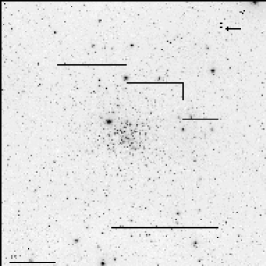
Figure 1: Finding chart of the area under study. The covered area is marked in black on an image of a plate (POSSI.E -optical R-.DSS1.486-LOW) plotted with Aladin (Bonnarel et al., 2000). The $H_{\beta}$ spatial coverage is limited to the central region. See text for details.

2.2 Reduction and Transformation

The reduction of the photometry is explained in length at Balaguer-Núñez et al. (2004a). Having the standard stars in the same images, the process is, in this case, equivalent to performe differential photometry.

Our general procedure has been to routinely obtain twilight sky flats for all the filters and a sizeable sample of bias frames (around 10) before and/or after every run. Flat fields are typically fewer in number, from five to ten per filter. Two or three dark frames of 2000 s were also taken. IRAF routines were used for the reduction process. The bias level was evaluated individually for each frame by averaging the counts of the most stable pixels in the overscan areas. The 2-D structure of the bias current was evaluated from the average of a number of dark frames with zero exposure time. Dark current was found to be negligible in all the cases. Flatfielding was performed using sigma clipped, median stacked, dithered twilight flats. Ten short exposures in every filter were taken every night with a magnitude limit of $V$$\sim$ 19. At least one exposure per filter was pointed to make the centre of the cluster fall on each of the WFC chips.

Our fields are not crowded. Thus, the synthetic aperture technique provides the most efficient measurements of relative fluxes within the frames and from frame to frame. We used the appropiate IRAF packages, and DAOPHOT and DAOGROW algorithms (Stetson, 1987, 1990). We analyzed the magnitude growth curves and determined the aperture correction with the IRAF routine MKAPFILE.

For WFC images from the INT, we employ the pipeline specifically developed by the Cambridge Astronomical Survey Unit. The process bias subtracts, gain corrects and flatfields the images. Catalogues are generated using algorithms described in Irwin (1985). The pipeline gives accurate positions in right ascension and declination linked to the USNO2 Catalogue (Monet et al., 1998), and instrumental magnitudes with their corresponding errors. A complete description can be found in Irwin & Lewis (2001) and in http://www.ast.cam.ac.uk/~wfcsur/index.php.

Table 2: Number of stars observed ($N$) and mean internal errors ($\sigma$) as a function of apparent visual magnitude.

$V$ range	$V$		$(b-y)$		$m_{1}$		$c_{1}$		$H_{\beta}$
	$N$	$\sigma$	$N$	$\sigma$	$N$	$\sigma$	$N$	$\sigma$	$N$	$\sigma$
8- 9	3	0.029	3	0.028	3	0.029	2	0.004
9-10	8	0.008	7	0.007	6	0.008	7	0.007	2	0.001
10-11	22	0.003	22	0.002	22	0.003	22	0.005	10	0.009
11-12	28	0.004	28	0.022	26	0.003	26	0.005	14	0.016
12-13	114	0.004	114	0.003	114	0.004	114	0.005	56	0.009
13-14	199	0.003	199	0.003	198	0.004	197	0.006	75	0.015
14-15	240	0.020	239	0.005	238	0.006	237	0.009	63	0.016
15-16	277	0.007	277	0.010	275	0.011	269	0.018	57	0.019
16-17	299	0.011	299	0.015	272	0.021	233	0.031	10	0.016
17-18	307	0.021	306	0.029	245	0.041	109	0.043	1	0.033
18-19	259	0.040	259	0.058	130	0.073	46	0.059
19-20	75	0.093	75	0.125	18	0.141	12	0.106
Total	1831		1828		1547		1274		288

The coefficients of the transformation equations were computed by a least squares method using the instrumental magnitudes of the standard stars and the standards magnitudes and colours in the $uvby-H_{\beta}$ system. Up to 68 standard stars in the field of the cluster (Nissen et al. 1987) were used depending on the size of the frame. Those standard stars with residuals greater than 2$\sigma$ were rejected. The reduction was performed for each night independently and in two steps. The first step is to determine the extinction coefficients for each passband from the standard stars. With the extinction coefficients fixed, the transformation coefficients to the standard system were fitted. The final errors as a function of apparent visual magnitude are given in Table LABEL:error67 and plotted in Fig. 2.

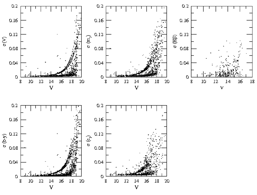
Figure 2: Mean internal errors of magnitude and colours (including the effects both from the instrumental measurements and the transformation uncertainties) as a function of the apparent visual magnitude, $V$, for all observed stars in the cluster region. The structure in the magnitude dependence is mainly owed to different numbers of measurements for individual stars since the centre of the cluster was shifted to be observed by each of the four CCD chips.

Table 3 lists the $u,v,b,y,H_{\beta}$ data for all 1843 stars observed in a region of 50$\arcmin$$\times$50$\arcmin$ around the open cluster M 67 (Fig. 1). Star positions are given as frame ($x,y$) and equatorial ($\alpha_{\mathrm{J}2000}$,$\delta_{\mathrm{J}2000}$) coordinates. An identification number was assigned to each star following the order of increasing right ascension. Column 1 is the ordinal star number; cols. 2 and 3 are $\alpha_{\mathrm{J}2000}$ and $\delta_{\mathrm{J}2000}$; cols. 4 and 5 are the respective $x$, $y$ coordinates in arcmin (arbitrary origin, close to cluster centre); cols. 6 and 7 are the $(b-y)$ and its error, cols. 8 and 9 the $V$ magnitude and its error, cols. 10 and 11 the $m_{1}$ and its error, cols. 12 and 13 the $c_{1}$ and its error, and cols. 14 and 15 the $H_{\beta}$ and its error. In col. 16, stars considered candidate members (see Sect. 4.1.) are labelled ’M’, while those classified as non-members show the label ’NM’.

The cross-identification of stars in common with the astrometry (Zhao et al., 1993), BDA (htpp://obswww.unige.ch/WEBDA), Sanders (1977), Hipparcos (ESA, 1997), Tycho-2 (Hog et al., 2000) and USNO-2 (Monet et al., 1998) catalogues is provided in Table 4.

2.3 Comparison with Previous Photometry

After Nissen et al. (1987), few studies of this cluster have been done in Strömgren photometry. Anthony-Twarog (1987) used a CCD to cover a larger area with up to 44 stars in common with our sample. Comparing Anthony-Twarog’s data with ours, the mean differences in the sense ours minus others, we get $-$0.01($\sigma$ = 0.04) in $V$, 0.00(0.02) in $b-y$, 0.00(0.04) in $m_{1}$ and 0.00(0.04) in $c_{1}$. The data published by Joner & Taylor (1997), with 14 stars in common with our catalogue, up to a limit of $V\sim$ 13, give differences of 0.01(0.03) in $V$, 0.01(0.02) in $b-y$, $-$0.02(0.03) in $m_{1}$ and $-$0.01(0.04) in $c_{1}$. Before Nissen et al. (1987), the study of Strom et al. (1971) with 19 common stars up to a limit of $V\sim$ 13.5 gives: $-$0.02(0.03) in $V$, $-$0.03(0.02) in $b-y$, 0.03(0.05) in $m_{1}$, $-$0.02(0.06) in $c_{1}$ and $-$0.02(0.07) in $H_{\beta}$, but a large scatter and a probable colour term in their results was already noted by Nissen et al. (1987).

The $V$ magnitude derived from the $y$ filter can be compared to the published broadband data. Several studies of M 67 give us mean differences in $V$, in the sense ours minus others (see Table LABEL:CompV67). Looking at the differences, one concludes that there are no apparent systematic trends in our photometry.

Table 5: Comparison of the $V$ magnitude to the published broadband data.

Author		$\Delta V_{\rm our-oth}$		$\sigma$	$N$
Eggen & Sandage (1964)	photoel.	$-$0.	02	0.04	173
Sanders (1989)	photoel.	0.	01	0.05	225
Gilliland et al. (1993)	CCD	$-$0.	02	0.03	136
Montgomery et al. (1993)	CCD	$-$0.	01	0.05	967
Kim et al. (1996)	CCD	$-$0.	01	0.04	89
Henden (2003)	CCD	0.	01	0.06	306
Sandquist (2004)	CCD	0.	01	0.03	154

3 Astrometric Analysis

We have studied the membership segregation using parametric and non-parametric approaches in the same way as in Balaguer-Núñez et al. (2004b); Balaguer-Núñez et al. (2005). Thanks to the proper motions obtained by Zhao et al. (1993) from high-quality plates taken with the double astrograph at the Zǒ-Sè station of the Shanghai Observatory, as in the case of NGC 1817 and NGC 2548, we have been able to use the same procedure in a very homogeneous way. The focal length of the Gautier 40 cm double astrograph at the Zǒ-Sè station is 6.9 m (hence a plate scale of 30″ mm^-1). All the plates were measured using the Photometric Data Systems model 1010 automatic measuring machine at the Purple Mountain Observatory in Nanjing. Zhao et al. give relative proper motions of 1046 stars within a 1$\aas@@fstack{\circ}$5 $\times$ 1$\aas@@fstack{\circ}$5 area, from measurements of 9 plates. The plates have a maximum epoch difference of 80 years.

Zhao et al. (1993) applied the plate-pair technique adopted many times at Shanghai Observatory to derive the relative proper motions. All linear and quadratic coordinate-dependent terms and the coma term were included in the plate-pair solution. The quoted mean errors of the relative proper motions vary from 0.4 mas yr^-1 for bright stars in the inner part of the cluster field to some 1.5 mas yr^-1 for faint stars in the outer part of the cluster. The comparison with the proper motions of Sanders (1977) and Girard et al. (1989) shows a satisfactory agreement. The magnitude limit of Zhao et al.’s study is $V\sim$ 15.5.

There are 50 stars in common with the Tycho-2 Catalogue (Hog et al., 2000). From their absolute proper motions we can calculate the transformation of Zhao et al.’s relative proper motions ($\mu_{x},\mu_{y}$) to the absolute reference frame:

$(\mu_{\alpha}\cos\delta)_{\mathrm{TYC2}}$ = $-6.510\ ({\pm}0.259)+1.013\ ({\pm}0.034)\cdot\mu_{x}-0.017\ ({\pm}1.644)\cdot\mu_{y}$;
$r$ = $0.956$; $N$ = 44
$(\mu_{\delta})_{\mathrm{TYC2}}$ = $-8.051\ ({\pm}0.404)+0.025\ ({\pm}0.056)\cdot\mu_{x}+0.957\ ({\pm}0.056)\cdot\mu_{y}$;
$r$ = $0.951$; $N$ = 50

where $r$ is the correlation coefficient and proper motions are expressed in mas yr^-1. The transformations show a rather good alignment of $x$- and $y$-axis with right ascension and declination, respectively.

Membership determination in Zhao et al. (1993) was calculated with an 8-parametric Gaussian model, and a list of stars with probability higher than 0.8 and a distance to the centre less than 45$\arcmin$ gave 282 cluster members. For the sake of coherence with our analysis of NGC 1817 and NGC 2548 (Balaguer-Núñez et al., 2004b; Balaguer-Núñez et al., 2005), we apply a 9-parametric Gaussian model and a non-parametric method to the proper motions obtained by Zhao et al. In contrast to their approach to the segregation of cluster members, we do not use any spatial information. Selecting members on kinematic and photometric criteria leaves the spatial information untouched, ready for a clean interpretation of radial and spatial trends.

Zhao et al. give $x,y$ coordinates, relative proper motions with their errors, number of plates used for proper motion determination, and cross-identifications with Sanders (1977). The authors state that their $x,y$ coordinates are taken from one of the plates, but a detailed analysis of the data shows that this is the case for the majority of the stars, but there is a small subset (61 stars) whose $x,y$ coordinates seem to have been taken from at least two other plates, and this introduces shifts in their quoted positions. Fortunately, Zhao et al.’s cross-identifications with Sanders (1977) were correct, what allowed us a complete cross-identification of our photometric catalogue with the proper motion data not losing any star. This inhomogeneity in Zhao et al. (1993) $x,y$ data does not affect our results, since we do not use these coordinates in our study. All tests performed show that Zhao et al.’s proper motions are not affected. The mistake in the $x,y$ coordinates of 61 stars seems to have been introduced in the final preparation of the tables by Zhao et al. (1993).

3.1 Membership probability: general frame

Let’s consider any observational plane ($a,b$), where $a$ and $b$ stand for any physical magnitudes. The distribution of any stellar sample on this plane can be described by its frequency function, $\Psi(a,b)$, measured in units of number of stars per unit area. The integral of the frequency function all over the plane, i.e., its volume, gives the number of members of the sample, $N$.

If the frequency fuction is normalised to unit volume, then we get the probability density function (PDF), $\psi(a,b)=\Psi(a,b)/N$, measured in units of fractions of the sample per unit area.

If two populations are superposed on the same region of the observational plane, but following different frequency functions $\Psi_{1}$ and $\Psi_{2}$, then, for any point ($a,b$) on that plane, it is possible to compute the probability $P$ for a star placed at that point to belong to population $i\;\;(i=1,2)$:

$$P=\frac{\Psi_{i}(a,b)}{\Psi_{1}(a,b)+\Psi_{2}(a,b)}.$$ (1)

For our purposes, ($a,b$) are the proper motions and the observational plane is then called the vector-point diagram (VPD).

Table 6: Distribution parameters and their uncertainties from a 9-parametric Gaussian model applied to M 67 cluster and the field. $n_{\rm c}$ measures the volume of the cluster frequency function ($n_{\rm f}=1-n_{\rm c}$), $\mu_{x}$ and $\mu_{y}$ are the mean relative proper motions, $\sigma_{\rm c}$, and $\sigma_{\mu_{x}}$ and $\sigma_{\mu_{y}}$ are the dispersions of the Gaussians fitted to the cluster and field distributions, and $\rho$ is the correlation for the field function (it fixes the orientation of the field elliptical function). The units of $\mu$ and $\sigma$ are mas yr^-1.

	$n_{\rm c}$	$\mu_{x}$	$\mu_{y}$	$\sigma_{\rm c}$	$\sigma_{\mu_{x}}$	$\sigma_{\mu_{y}}$	$\rho$
M 67	0.364	$-$0.59	0.49	0.89
	$\pm 0.016$	$\pm 0.07$	$\pm 0.06$	$\pm 0.05$
field		0.02	3.31		9.00	8.63	$-0.21$
		$\pm 0.10$	$\pm 0.48$		$\pm 0.03$	$\pm 0.24$	$\pm$0.02

3.2 The classical approach

The parametric method assumes the existence of two populations in the VPD: cluster and field. The corresponding frequency functions are modelled as parametric Gaussian functions: a circular Gaussian model is adopted for the cluster distribution, while a bivariate (elliptical) Gaussian is admitted to describe the field. We apply a 9-parametric Gaussian model following Balaguer-Núñez et al. (2004b, 2005) and the results are shown in Table LABEL:para67. Our implementation takes into account the individual errors of the proper motion measurements (Zhao & He, 1990). If we transform the obtained mean relative proper motion of the cluster to the absolute system by the equations above, we get ($\mu_{\alpha}\cos\delta,\mu_{\delta}$) = ($-$7.1$\pm$0.8,$-$7.6$\pm$0.4) mas yr^-1.

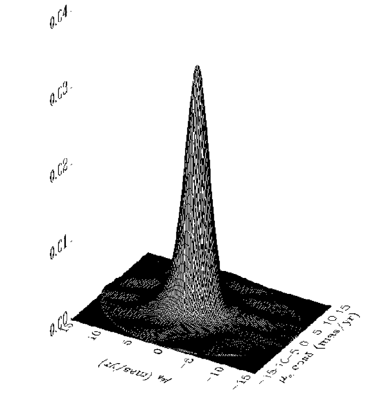
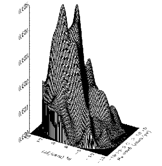
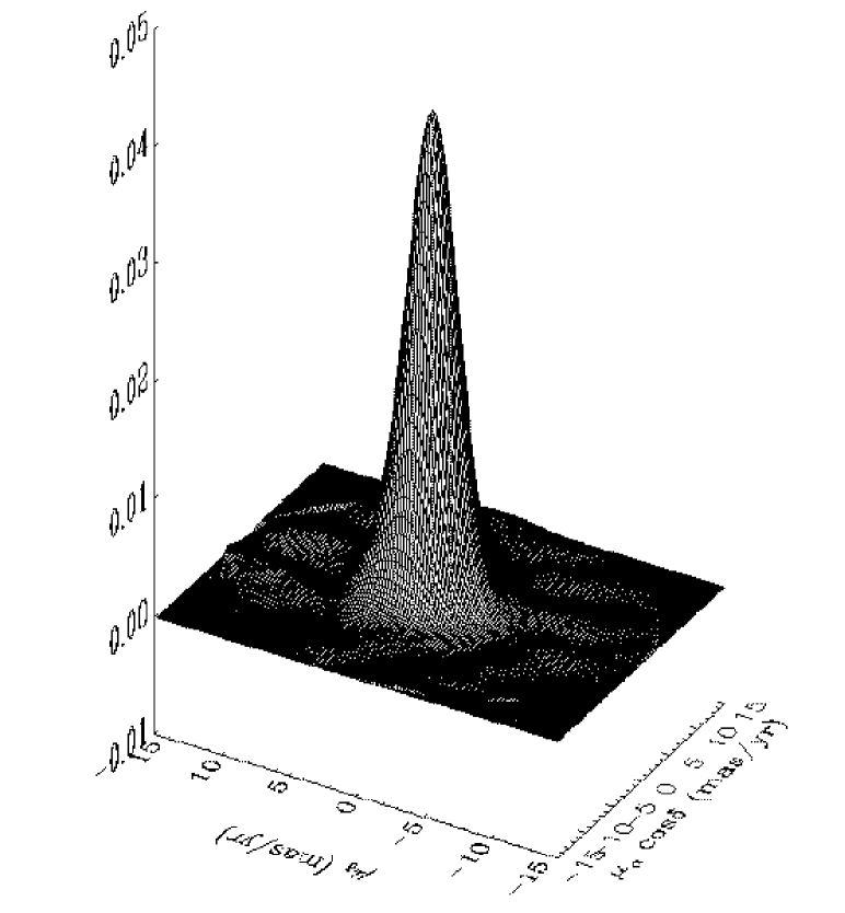
Figure 3: Empirical PDFs in the vector-point diagram. Top: $\psi_{\rm c+f}$ mixed sample from the inner circle of 35’ centred on the point of maximum spatial density of stars. Centre: $\psi_{\rm f}$ field population from outside this circle. Bottom: $\psi_{\rm c}$ cluster population of M 67. It is noticeable that the cluster lies on a poorly populated background field.

3.3 The non-parametric approach

The cluster/field segregation from astrometry has also been analysed with a non-parametric approach, as explained in length in Balaguer-Núñez et al. (2004b); Balaguer-Núñez et al. (2005). We perform an empirical determination of the frequency functions from the vector-point diagram (VPD), without relying on any previous assumption about their profiles. In the area occupied by the cluster, the frequency function $\Psi_{\rm c+f}$ is made up of two contributions: cluster, $\Psi_{\rm c}$, and field, $\Psi_{\rm f}$. To disentangle the two populations, we studied the VPD for the plate area outside a circle centred on the cluster. To this end, the centre of the cluster was chosen as the point of highest spatial density. The only two assumptions that we need to apply are (1) that it is possible to determine the frequency function of the field stars from some spatial area free of cluster members (outside the circle in our case); and, (2) that this frequency function is representative of the field frequency function in the area occupied by the cluster.

We did tests with circles of very different radii searching a reasonable tradeoff between cleanness (absence of a significant amount of cluster members) and signal-to-noise ratio (working area not too small, to avoid small number statistics). The kernel density estimator technique (Hand 1982) was applied in the VPD to these data. Details of the procedure can be found in Galadí-Enríquez et al. (1998). Circular Gaussian kernel functions were used, with Gaussian dispersion (also called smoothing parameter) $h$ elected according to Silverman’s rule (Silverman 1986). This way, the empirical frequency functions were computed for a grid with cell size of 0.2 mas yr^-1, well below the proper motion errors. The procedure was tested for several subsamples applying different proper motion cutoffs and the adopted one, as in the cases of NGC 1817 and NGC 2548, is of $|\mu|\leq$ 15 mas yr^-1.

We finally find that the area outside a circle with a radius of 35$\arcmin$ centred on the cluster yields a clean frequency function with low cluster contamination and low noise. We can scale this field frequency function to represent the field frequency function in the inner circle, $\Psi_{\rm f}$, by simply applying a factor linked to the area. The cluster empirical frequency function can then be determined as $\Psi_{\rm c}$ = $\Psi_{\rm c+f}-\Psi_{\rm f}$. Normalizing the frequency functions to volume unity we get the probability density functions for the mixed population (inside the circle), for the field (outside the circle) and for the cluster (non-field) population. These PDFs are displayed in Figure 3. We estimate the typical noise level, $\gamma$, present in the result and we restricted the probability calculations to the stars with cluster PDF $\geq$ 3$\gamma$.

The maximum of the cluster PDF is located at ($\mu_{x},\mu_{y}$) = ($-$0.6$\pm$0.2,0.4$\pm$0.2) mas yr^-1, which coincides well with the values obtained in the parametric method. If we transform this value to the absolute system, we get an absolute proper motion for the cluster of ($\mu_{\alpha}\cos\delta,\mu_{\delta}$) = ($-$7.1$\pm$0.7,$-$7.7$\pm$0.5) mas yr^-1. Thirty six out of the 50 Tycho-2 stars are classified as members giving a mean value of ($\mu_{\alpha}\cos\delta,\mu_{\delta}$) = ($-$8.4$\pm$2.1,$-$6.1$\pm$2.2) mas yr^-1. This is fully compatible with our result, but we consider our figures more reliable, since they are derived from the whole sample of stars.

3.4 Results and discussion

The non-parametric approach does not take into account the errors of the individual proper motions. But the full width at half maximum (FWHM) of the PDF of the cluster gives an estimation of the width of the distribution. We obtained a FWHM of $\sim$4.1$\pm$0.2 mas yr^-1. Taking into account the Gaussian dispersion owed to the smoothing parameter $h\leavevmode\nobreak\ =$ 1.34 mas yr^-1, this would correspond to a r.m.s. error on proper motions of 1.55 mas yr^-1. But from Zhao et al. (1993) we know that the mean proper motion precision is 1.24 mas yr^-1, what gives us an intrinsic dispersion component of 0.93 mas yr^-1, of the same order that the value obtained by the parametric membership determination ($\sigma_{c}$ = 0.89$\pm$0.05 mas yr^-1, $\sim$ 4 km s^-1 at the distance of 900 pc).

Figure 4: The histogram of cluster membership probability of M 67. The solid line gives the results for classical parametric method $P_{\rm P}$ (Section 3.2), while the dotted line corresponds to the non-parametric approach $P_{\rm NP}$ (Section 3.3). The arrows mark the limiting probabilities for member selection for each method.

Membership probabilities are computed according to Eq. 1, both from the classical, parametric frequency functions ($P_{\rm P}$) and from the non-parametric, empirical frequency funcions ($P_{\rm NP}$). The cluster membership probability histogram (Figure 4) shows a clear separation between cluster members and field stars in both approaches (the solid line being the classical parametric method, dotted line the non-parametric approach). The non-parametric technique yields an expected number of cluster members from the integrated volume of the cluster frequency function in the VPD areas of high cluster density, where PDF$\geq$ 3$\gamma$. The expected amount of cluster members in this VPD area is of 393. Sorting the sample in order of decreasing non-parametric membership probability, $P_{\rm NP}$, the first 393 stars are the most probable cluster members. The minimum value of the non-parametric probability (for the 393-rd star) is $P_{\rm NP}\leavevmode\nobreak\ =0.87$.

To decide where to set the limit among members and non-members in the list sorted in order of decreasing parametric membership probability, $P_{\rm P}$, we accept the size of the cluster predicted by the non-parametric method, 393 stars. Thus we consider that the 393 stars of highest $P_{\rm P}$ are the most probable members, according to the results of the parametric technique. The minimum value of the parametric probability (for the 393-rd star) is $P_{\rm P}\leavevmode\nobreak\ =0.55$. It is worth noting that, contrary to what happened with the previous two clusters studied by us, and in other cases found in the literature (Galadí-Enríquez et al., 1998), in this case the original parametric segregation (Zhao et al., 1993) at $P_{\rm P}>0.8$ was underestimating, and not overestimating, the number of probable members. This is because M 67 is much more populated, and displays a higher constrast against the field, than the other clusters. The need to reach a $P_{\rm P}$ cutoff much lower than the $P_{\rm NP}$ cutoff illustrates the effects of an imperfect modelling of the wings of the real distribution in the parametric method. Also, the importance of having some objective criterium to decide the $P_{\rm P}$ cutoff is evident from our results.

With these limiting probabilities ($P_{\rm NP}\geq 0.87$; $P_{\rm P}\geq 0.55$), we get a 97$\%$ (1014 stars) of agreement in the segregation yielded by the two methods. Table 7 lists the cross-identifications with Zhao et al. (1993) and Sanders (1977), the $P_{\rm P}$ and the $P_{\rm NP}$ for the 1046 stars.

As in Balaguer-Núñez et al. (2004b), we accept as probable members those stars classified as member by at least one of the two methods. This way we get a list of 412 astrometric probable member stars. Figure 5 shows the proper motion VPD and the sky distribution for all the measured stars, where empty circles denote an astrometric probable member of M 67, and all other stars are considered field stars and they are indicated by dots.

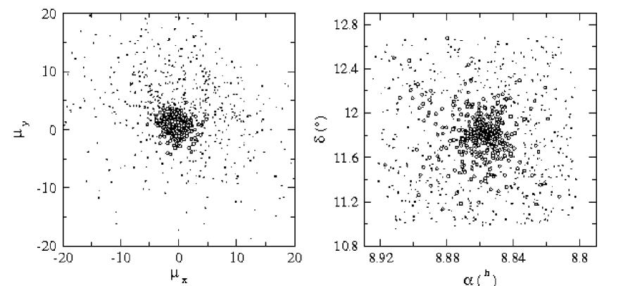
Figure 5: The proper motion vector-point diagram (VPD) and spatial distribution of stars in M 67 region (empty circles for the astrometric probable members of M 67 and dots for field stars). Units of relative proper motions are mas yr^-1.

A comparison of the cluster/field segregation for the 143 stars in common with the radial velocity studies by Mathieu et al. (1986, 1990) is given in Tables 8 (candidate members) and 9 (non-members). The radial velocities have typical standard deviations for a set of measurements of any given star that range between 0.5 and 0.8 km s^-1. To quantify the differences in the segregation, we do as in Balaguer-Núñez et al. (2004b); Balaguer-Núñez et al. (2005) and set an agreement index $P_{\rm c}$ to 1 if the parametric probability, $P_{\rm P}$, agrees with the radial velocity segregation, 2 if the non-parametric probability, $P_{\rm NP}$, agrees, 3 if both probabilities, $P_{\rm P}$ and $P_{\rm NP}$, agree and 0 if none does. We find 125 out of 143 stars with $P_{\rm c}>$ 0, that is 87$\%$ agreement with the radial velocities segregation. This 13$\%$ of disagreement consists of 15 stars out of 41 being considered non-members on the basis of proper motions, while only 3 out of 102 were found to be astrometric members but considered non-members on the basis of radial velocities. Those three have only one measurement of their radial velocities and two of them are known to be spectroscopic binaries (SB), therefore the measurement may be different from the systemic velocity and thus they cannot be completely ruled out as members.

If we compare the parametric and non-parametric methods, the behaviour is rather similar. For the parametric method we find a total of 121 stars (85$\%$) whose membership assignation coincides with the radial velocity criterion, while for the non-parametric method this amounts to 124 stars (87$\%$).

Table 8: The cross-identification of stars considered as candidate members by us, with the radial velocities sudies by Mathieu et al. (1986, 1990) and the comparison of those with the parametric ($P_{\rm P}$) and non-parametric ($P_{\rm NP}$) probabilities. See text for explanation of the agreement index $P_{\rm c}$.

IDBDA	IDZhao	$P_{\rm P}$	$P_{\rm NP}$	$P_{\rm c}$	$Vr^{*}$	IDBDA	IDZhao	$P_{\rm P}$	$P_{\rm NP}$	$P_{\rm c}$	$Vr^{*}$
4	818	0.94	0.96	3	34.0 $\pm$2.0	185	958	0.79	0.94	3	33.4 $\pm$0.0
16	829	0.88	0.96	3	33.2 $\pm$0.9	190	989	0.80	0.94	0	43.6 $\pm$0.0 SB
18	521	0.92	0.95	3	32.9 $\pm$0.5	192	603	0.98	0.97	3	32.7 $\pm$1.1
20	834	0.96	0.97	3	33.1 $\pm$1.0	193	999	0.98	0.97	3	33.7 $\pm$0.5
22	839	0.95	0.96	3	34.4 $\pm$1.9 SB1	195	1017	0.97	0.98	3	33.87$\pm$0.12 SB1
28	840	0.97	0.97	3	33.7 $\pm$1.0	210	1005	0.98	0.97	3	33.9 $\pm$1.1
30	845	0.97	0.97	3	33.6 $\pm$0.4	215	608	0.98	0.98	3	33.6 $\pm$0.6
37	846	0.97	0.97	3	33.7 $\pm$0.3	216	1010	0.97	0.98	3	33.03$\pm$0.13 SB1
46	843	0.98	0.97	3	33.8 $\pm$0.1	217	1002	0.97	0.97	3	33.3 $\pm$0.4
48	848	0.96	0.98	3	33.0 $\pm$0.4	218	1006	0.98	0.97	3	34.0 $\pm$0.5
51	849	0.96	0.97	3	34.6 $\pm$0.9	219	1007	0.98	0.98	3	33.4 $\pm$0.3 SB1
54	863	0.95	0.97	3	34.5 $\pm$0.7	223	609	0.68	0.94	3	32.8 $\pm$0.4
55	862	0.75	0.92	0	42.1 $\pm$0.0 SB	224	1011	0.95	0.96	3	32.55$\pm$0.07 SB1
72	876	0.97	0.98	3	33.3 $\pm$0.6	226	1013	0.98	0.98	3	32.5 $\pm$1.0
79	860	0.97	0.98	3	34.1 $\pm$1.7	227	1004	0.98	0.97	3	32.8 $\pm$0.7
84	966	0.78	0.94	3	34.1 $\pm$0.4	231	1029	0.97	0.97	3	32.5 $\pm$0.6
86	933	0.81	0.86	1	27.6 $\pm$0.0	236	1025	0.98	0.98	3	33.82$\pm$0.18 SB1
88	927	0.96	0.97	3	34.13$\pm$0.23 SB2	237	611	0.97	0.98	3	34.7 $\pm$0.7
95	886	0.98	0.98	3	34.7 $\pm$2.4	238	1028	0.75	0.94	3	38.3 $\pm$0.0
96	929	0.96	0.98	3	33.1 $\pm$0.7	241	1027	0.96	0.96	3	33.2 $\pm$0.7
101	930	0.97	0.98	3	32.9 $\pm$0.9	243	1026	0.96	0.96	3	33.4 $\pm$0.5
102	893	0.98	0.97	3	36.17$\pm$0.17 SB1	244	1032	0.93	0.96	3	33.55$\pm$0.05 SB1
104	931	0.95	0.97	3	33.5 $\pm$0.4	248	612	0.98	0.98	3	34.0 $\pm$1.3
105	883	0.80	0.94	3	34.3 $\pm$0.7	252	618	0.97	0.96	3	32.5 $\pm$1.0
108	894	0.51	0.93	2	34.7 $\pm$0.6	255	1043	0.96	0.97	3	31.3 $\pm$0.3
111	891	0.98	0.97	3	33.70$\pm$0.22 SB1	256	226	0.96	0.98	3	33.2 $\pm$0.9
115	918	0.97	0.98	3	34.4 $\pm$0.5	262	1046	0.97	0.97	3	31.6 $\pm$0.7
117	887	0.98	0.98	3	34.4 $\pm$0.3 SB2	266	647	0.78	0.94	3	34.3 $\pm$0.4
119	924	0.97	0.97	3	34.34$\pm$0.21 SB2	271	1058	0.93	0.96	3	34.1 $\pm$0.8
124	912	0.97	0.98	3	29.6 $\pm$0.7 SB	272	645	0.97	0.97	3	31.8 $\pm$0.4
127	911	0.97	0.98	3	33.3 $\pm$0.8	281	1060	0.96	0.97	3	33.4 $\pm$0.8
130	910	0.94	0.98	3	33.7 $\pm$0.7	286	697	0.35	0.92	2	33.6 $\pm$0.5
131	972	0.95	0.96	3	33.3 $\pm$2.0 SB2	287	698	0.98	0.97	3	32.8 $\pm$0.5
134	907	0.98	0.97	3	32.5 $\pm$1.2 SB1	289	683	0.94	0.96	3	32.7 $\pm$0.4
135	908	0.97	0.97	3	34.3 $\pm$0.6	291	700	0.96	0.97	3	34.1 $\pm$0.1
136	974	0.94	0.96	3	32.87$\pm$0.12 SB1	305	133	0.52	0.92	2	34.2 $\pm$0.9
141	947	0.86	0.95	3	33.6 $\pm$0.4	1182	174	0.95	0.98	3	34.6 $\pm$0.9
143	937	0.91	0.96	3	32.93$\pm$0.07 SB1	2079	172	0.98	0.98	3	34.4 $\pm$0.5
149	949	0.98	0.97	3	35.5 $\pm$0.8	2087	211	0.94	0.97	3	31.5 $\pm$3.0
151	971	0.81	0.94	3	33.9 $\pm$0.5	3035	1001	0.98	0.98	3	34.1 $\pm$0.5
157	976	0.98	0.98	3	33.6 $\pm$0.5	3116	642	0.98	0.97	3	33.60$\pm$0.13 SB1
163	995	0.98	0.98	3	33.8 $\pm$0.8	4004	939	0.98	0.98	3	33.48$\pm$0.19 SB2
164	983	0.79	0.94	3	33.3 $\pm$0.4	4096	578	0.97	0.97	3	34.0 $\pm$0.8
166	4	0.97	0.98	3	33.3 $\pm$0.3	7591	135	0.91	0.96	3	33.4 $\pm$0.8
170	953	0.60	0.93	3	33.59$\pm$0.10 SB1	7657	505	0.28	0.87	2	33.2 $\pm$0.9
174	961	0.97	0.98	3	36.2 $\pm$4.5	8402	231	0.83	0.94	3	33.6 $\pm$0.4
176	914	0.97	0.98	3	32.5 $\pm$0.4 SB1	8524	639	0.69	0.89	3	33.6 $\pm$0.7
180	985	0.98	0.97	3	35.0 $\pm$0.8	8571	253	0.94	0.95	3	34.2 $\pm$0.4
181	955	0.98	0.98	3	33.3 $\pm$0.7	8792	282	0.85	0.93	3	33.1 $\pm$0.5
182	956	0.97	0.98	3	32.2 $\pm$2.2	8808	277	0.85	0.94	3	29.6 $\pm$1.0
184	987	0.98	0.97	0	61.4 $\pm$0.0	8832	713	0.97	0.97	3	33.5 $\pm$0.7

(*) Zero errors mean that only one measurement was taken and no dispersion could be calculated. SB1: Single-lined spectroscopic binary. SB2: Double-lined spectroscopic binary.

Table 9: The same as Table 8, for stars considered as non-members by us.

IDBDA	IDZhao	$P_{\rm P}$	$P_{\rm NP}$	$P_{\rm c}$	$Vr^{*}$	IDBDA	IDZhao	$P_{\rm P}$	$P_{\rm NP}$	$P_{\rm c}$	$Vr^{*}$
8	822	0.00	0.70	3	29.1 $\pm$1.8	7116	27	0.00	0.00	3	13.7 $\pm$0.0
10	136	0.00	0.00	3	16.3 $\pm$0.0	7232	52	0.00	0.00	3	4.2 $\pm$0.0
45	857	0.00	0.00	3	-14.0 $\pm$0.0	7251	434	0.00	0.47	0	34.56$\pm$0.14 SB1
49	3	0.00	0.00	3	28.1 $\pm$0.0	7335	75	0.00	0.00	3	-18.9 $\pm$0.0
144	951	0.00	0.00	0	33.72$\pm$0.14 SB1	7350	72	0.00	0.00	3	-13.0 $\pm$0.0
155	943	0.00	0.00	3	3.6 $\pm$1.0	7378	458	0.00	0.00	3	57.8 $\pm$0.0
173	963	0.00	0.00	0	33.37$\pm$0.20 SB1	7434	94	0.00	0.65	0	33.7 $\pm$0.9
200	601	0.00	0.00	3	12.0 $\pm$0.4	7440	98	0.00	0.00	3	14.95$\pm$0.11 SB1
206	602	0.00	0.00	0	34.8 $\pm$0.3	7445	85	0.00	0.72	0	33.8 $\pm$1.0
240	215	0.17	0.84	3	43.3 $\pm$0.15 SB1	7488	485	0.06	0.84	0	33.0 $\pm$0.3
242	1024	0.00	0.00	3	-1.1 $\pm$0.4	7515	489	0.06	0.84	3	27.6 $\pm$0.6
277	648	0.00	0.00	3	1.6 $\pm$0.0	7551	104	0.00	0.67	3	8.9 $\pm$0.0
2086	210	0.00	0.00	0	33.3 $\pm$0.6	7663	492	0.03	0.00	3	1.5 $\pm$0.0
3128	620	0.00	0.00	3	-20.7 $\pm$0.0	7674	496	0.00	0.00	0	33.7 $\pm$0.5
4166	481	0.00	0.00	3	-2.5 $\pm$0.0	8135	566	0.00	0.78	0	34.2 $\pm$0.4
4168	482	0.00	0.00	3	39.5 $\pm$0.4	8355	623	0.00	0.63	3	49.3 $\pm$0.0
6469	453	0.00	0.00	0	34.1 $\pm$0.2	8522	657	0.00	0.00	3	12.6 $\pm$0.0
6470	468	0.00	0.70	0	33.3 $\pm$0.3	8533	632	0.00	0.76	3	67.8 $\pm$0.5
6474	495	0.00	0.73	3	9.5 $\pm$0.6	8557	250	0.00	0.00	0	33.9 $\pm$0.5
6514	261	0.00	0.00	0	34.5 $\pm$0.7	9015	744	0.10	0.81	0	33.5 $\pm$1.6
7112	37	0.00	0.00	3	-9.0 $\pm$0.0

(*) Zero errors mean that only one measurement was taken and no dispersion could be calculated. SB1: Single-lined spectroscopic binary. SB2: Double-lined spectroscopic binary.

3.5 Magnitude effects in UCAC2 and proper motions as indicator of binarity

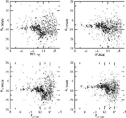
Figure 6: UCAC2 proper motion vs magnitude for M 67 area. Top row: $\mu_{\alpha}$ and $\mu_{\delta}$ vs the UCAC2 magnitude (Zacharias et al., 2004); bottom row: vs 2MASS $J$ magnitude (Skrutskie et al., 2006). Proper-motion errors are about 1–3 mas yr^-1 for stars to 12th magnitude, and about 4–7 mas yr^-1 for fainter stars up to 16th magnitude. UCAC2 proper motions are taken from Tycho-2 (Hog et al., 2000) catalogue down to its magnitude limit $V\sim$12. From this magnitude, and down to the limiting magnitude of our selection of candidate members (marked as empty circles), there is a systematic trend depicted with a thick line

The internal dynamics of non-resolved multiple systems could induce a motion of the measured photocentre different from the motion of the barycentre. This effect has to be null for equal-mass binaries and almost undetectable for binaries with components of extremely different masses, and should reach a maximum somewhere in between. When looking to the histogram of proper motion modules, this effect would skew the distribution inducing a longer tail towards high values.

Bica & Bonatto (2005) have made an attempt of identifying high-velocity stars as unresolved binary cluster members and, as a result, for mapping and quantifying the binary component in colour-magnitude diagrams. They analysed 9 open clusters using UCAC2 proper motions (Zacharias et al., 2004) and 2MASS photometry (Skrutskie et al., 2006). As a test case of the method, they use M 67. Their study of the modulus of the proper motion in the cluster area yields a double-peaked distribution instead of the skewed Gaussian that, in principle, could be expected. The authors associate the peaks to high-velocity and low-velocity populations in the cluster, and the high-velocity group is interpreted as produced by unresolved binary systems. This behaviour is found in the core and in the halo of the cluster. The authors claim internal dispersions of the order of $\sim$6 km s^-1 for single stars and around $\sim$11 km s^-1 for unresolved binaries, and a difference between the two peaks of more than 20$-$30 km s^-1. These strikingly unrealistic numbers and the lack of any error estimation adds suspicion to the fact that all the stars from the high-velocity peak are dimmer than $J\sim$ 12 (Fig. 6 in their paper), when the abundance of binaries among the bright members of M 67 is well known.

A similar study using the proper motions by Zhao et al. (1993) gives as a result a bell-shaped distribution with a tail towards higher velocities. We were not able to find a double-peaked distribution in the core nor in the halo. Different tries of dividing the distribution did not show any relation to binarity when checked on the corresponding colour-magnitude diagram.

As it is well depicted by the study of Platais et al. (2003), the presence of residual colour/magnitude terms in any proper motion analysis is almost unavoidable. This is specially true when one deals with an all-sky catalogue, where the proper motions are derived from different first epoch sources. Aware of these facts, we have checked for magnitude terms in UCAC2 (Zacharias et al., 2004) proper motions. We plot proper motion vs magnitude in Fig. 6. The UCmag magnitude in the top row is in the UCAC bandpass (579-642 nm, between $V$ and $R$) and should be considered approximate. UCAC2 proper motions are derived by using over 140 ground- and space-based catalogues, including Tycho-2 (Hog et al., 2000) and the AC2000.2 (Urban et al., 1998). In the bottom row, we have plotted the 2MASS $J$ magnitude as a double check of the results. Cluster member candidates from our selection are marked as empty circles. We can note how the UCAC2 proper motions of these stars show a trend with magnitude for magnitudes fainter than from $V\sim 12$, highlighted by the regression fit marked by a thick line. The behaviour detected by Bica & Bonatto (2005) is not related to binarity, but due to systematics in the proper motion data. The use of proper motion data from UCAC2 Catalogue should be carefully taken to avoid systematics.

4 Colour-Magnitude Diagrams

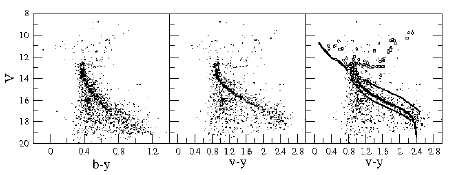
Figure 7: Colour-magnitude diagrams of the M 67 area. Figure on the right shows the astrometric probable members as empty circles. Thick line is a shifted ZAMS, with the chosen margin for candidate members ($V+0.5$,$V-1$) in thin lines. See text for details.

We use the $V$ vs $(v-y)$ colour-magnitude diagram for our study (Fig. 7 right and centre) because it defines the main-sequence of a cluster significantly better than the traditional $V$ vs $(b-y)$ diagram (Meibom, 2000) in presence of extinction. The colour-magnitude diagram of all the stars in the area displays a fairly well defined main sequence. The advanced age of this cluster is obvious at first sight looking at the diagram. Moreover, the sequence of binaries can be easily followed.

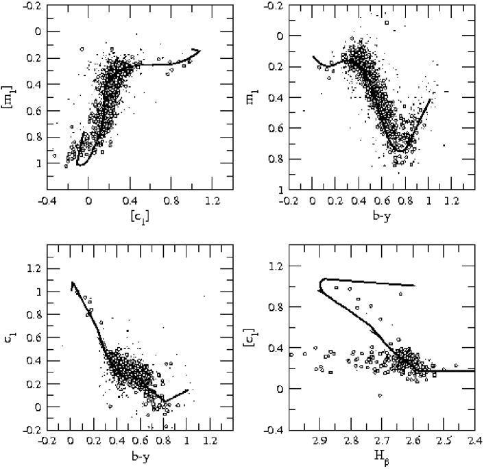
Figure 8: The colour-colour diagrams of M 67. Empty circles denote candidate members of M 67, chosen with astrometric and non-astrometric criteria as explained in Section 4.1. The thick line is the solar ZAMS standard relation shifted by $E(b-y)$ = 0.03 when necessary. Evolutionary and binarity effects are noticeable in these diagrams. Some of the candidate members, known to be multiple stars, have very discordant values.

4.1 Selection of candidate member stars

Unfortunately, proper motions are only available for the brightest stars in the area. Photometric measurements help to reduce the possible field contamination in the proper motion membership —among bright stars—, as well as to enlarge the selection of members towards faint magnitudes. Our astrometric segregation of member stars has a limiting magnitude of $V\sim$ 15.5. From this magnitude down to $V\sim 18$ we construct a ridge line following a fitting of the observational zero-age main sequence (ZAMS) (Crawford, 1975, 1978, 1979; Hilditch et al., 1983; Olsen, 1984), on the $V$ vs $(v-y)$ diagram. A selection of stars based on the distance to this ridge line is then performed. The width of the sequence defined by astrometric candidate members allows us to establish the margins for the selection of fainter stars. The chosen margin includes all the stars between $V+0.5$ and $V-1$ from the ridge line, as shown in the right panel of Fig. 7. This magnitude range allows for photometric errors in the two axis, intrinsic dispersion around the ZAMS and multiplicity effects. The interval of 1 magnitude at the bright side comprises the width of the sequence and is large enough to allow for equal-mass binaries ($\Delta V=0.75$) and for most triples ($\Delta V=1.19$ for equal-mass systems). The interval of 0.5 magnitudes at the faint side agrees with the observed width of the main sequence and is larger than the expected photometric errors. Luckily, the high density of M 67 and its outstanding contrast against the population of field stars (shown by the comparison of the density functions in Fig. 3) makes the fine-tuning of these margins to be non-critical: the number of non-members introduced by our choice is low, and the loss of true members is minimised.

Extreme outliers have been rejected making use of the colour-colour diagrams (Fig. 8) with the help of the standard relations (Crawford, 1975, 1978, 1979; Hilditch et al., 1983; Olsen, 1984). The astrometric and photometric selection gives a final set of 776 candidate members. They are plotted in Fig. 8 as filled circles in the $[m_{1}]-[c_{1}]$, $m_{1}-(b-y)$, $c_{1}-(b-y)$ and $[c_{1}]-H_{\beta}$ diagrams. This photometric selection is known to contain a certain amount of field contamination, reason why we prefer to talk about “candidate members”, rather than “bona fide members”. Anyhow, the selection done leads to a set of stars overwhelmingly dominated by true members: the methods applied in Sect. 5 to derive the physical parameters of the cluster are readily capable of extracting reliable mean values from such a sample.

5 Physical parameters of the cluster

The stars of the area selected as candidate cluster members were classified into photometric regions and its physical parameters determined, following the algorithm described in Masana et al. (2007) and Jordi et al. (1997). The algorithm uses $uvby-H_{\beta}$ photometry and standard relations among colour indices for each of the photometric regions of the HR diagram.

5.1 Distance, reddening and metallicity

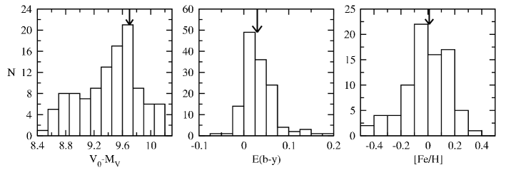
Figure 9: The histograms of the distance modulus, reddening and metallicity of the selected member stars of M 67 with $H_{\beta}$ measurements. The arrows indicate the mean values adopted for the cluster.

Only 251 stars among the 776 candidate members have $H_{\beta}$ measurements. So the computation of physical parameters is only possible for that subset. The results are shown in Fig. 9. Excluding peculiar stars and those with inconsistence among their photometric indices and applying an average with a 2$\sigma$ clipping to that subset, we found a mean reddening value of $E(b-y)$ = 0.03$\pm$0.03 (corresponding to $E(B-V)$ = 0.04) and a mean distance modulus of $V_{0}-M_{V}$ = 9.4$\pm$0.4. The distance modulus may be biased towards short values due to the presence of multiple stars treated as if they were single ones. A substantial fraction of binaries tend to have equal mass companions. These binaries would be well-separated from the cluster main-sequence, so they can be easily detected and removed. However, low mas ratio binaries would remain, and might systematically reduce the estimated distance since they are brighter and redder than single cluster members. If we set a conservative limit for stars with lower value than 9.4 in the distance modulus, we can see from the $V$ vs $b-y$ diagram that these lower values mainly correspond to stars above the main sequence of the cluster which are most probably multiple stars. Excluding those we can get a value of $V_{0}-M_{V}$ = 9.7$\pm$0.2 from the study of 66 stars that can be confidently considered singles.

Metallicity is better calculated studying only the 81 F and G type stars in our sample following Masana (1994). We find a mean value of [Fe/H] = 0.01$\pm$0.14.

5.2 Age

The publication by Clem et al. (2004) of empirically constrained colour-temperature relations in the Strömgren system makes possible an isochrone fitting to our results. The least unsatisfactory fitting is found for the Pietrinferni et al. (2004, 2006) tracks. Figure 10 shows the isochrones from Pietrinferni et al. (2004) for scaled solar models of solar metallicity and ages of 4.0, 4.2, 4.4 and 4.6 Gyr for models with overshooting and of 3.4, 3.6, 3.8 Gyr for canonical models. The addopted reddening and distance modulus are $E(b-y)$ = 0.03 and $V_{0}-M_{V}$ = 9.7; from Pietrinferni et al. (2006) for $\alpha$-enhanced models of solar metallicity and ages of 3.6, 3.8, 4.0 and 4.2 Gyr for models with overshooting and of 3.0, 3.2, 3.4 Gyr for canonical models. For this case, the addopted reddening and distance modulus are $E(b-y)$ = 0.05 and $V_{0}-M_{V}$ = 9.7. Empty circles are candidate members. Canonical models give lower ages. $\alpha$-enhanced models reproduce better the behaviour of the red giants clump and red giant branch, but seem to behave worse in the lower giants branch and subgiants branch where models with overshooting seem to give a better fit. It seems apparent that none of the models provides a good fit over all the areas of the colour-magnitude diagram. We decided to adopte a compromise between these isochrones and give an estimation of the age of $t$ = 4.2$\pm$0.2 Gyr ($\log t$ = 9.62$\pm$0.02) in agreement with previous estimates by other outhors.

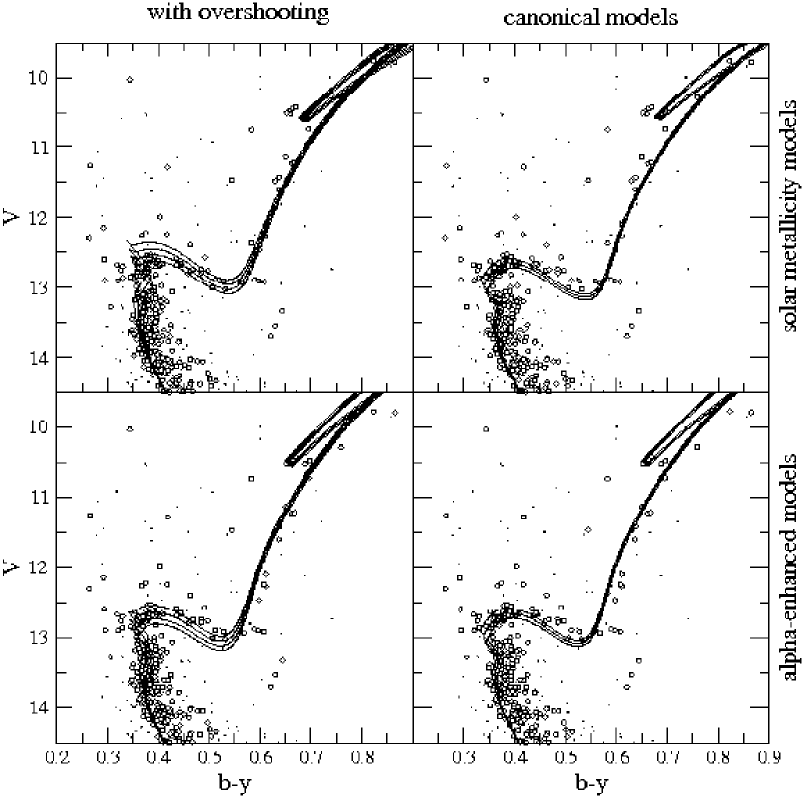
Figure 10: Isochrones from Pietrinferni et al. (2004) for scaled solar models (top row) of solar metallicity and ages of 4.0, 4.2, 4.4 and 4.6 Gyr for models with overshooting (left panel) and ages of 3.4, 3.6, 3.8 Gyr for canonical models (right panel). Isochrones from Pietrinferni et al. (2006) for alpha-enhanced models (bottom row) of solar metallicity and ages of 3.6, 3.8, 4.0 and 4.2 Gyr for models with overshooting (left panel) and ages of 3.0, 3.2, 3.4 Gyr for canonical models (right panel).

6 Multiple Star Systems, Blue Stragglers and other peculiars

6.1 Multiple Star Systems

The high binary content of M 67 was already noted by Racine (1971): “more than half of the M 67 main-sequence stars between G2 and K5 appear to be unresolved multiple stars”. Montgomery et al. (1993) studied the distribution of binaries and calculated a 22$\%$ of equal-mass component binaries. Trying to account for the binaries with low mass ratios when studying the distribution of multiple stars from a fiducial main sequence, they found a ratio of 38$\%$. Due to the possible presence of very low mass ratio binaries, this percentage is a lower limit. Fan et al. (1996) reconsidered the mass ratios and number of binaries in M 67, and using models leaving the mass ratio to randomly vary from zero to one, they found that the true binary fraction in this cluster depends critically on how to account for the contribution of low mass-ratio binaries. From the models, around a 50$\%$ of binaries seems a plausible scenario, with a binary mass ratio distribution more consistent with being random than double-peaked.

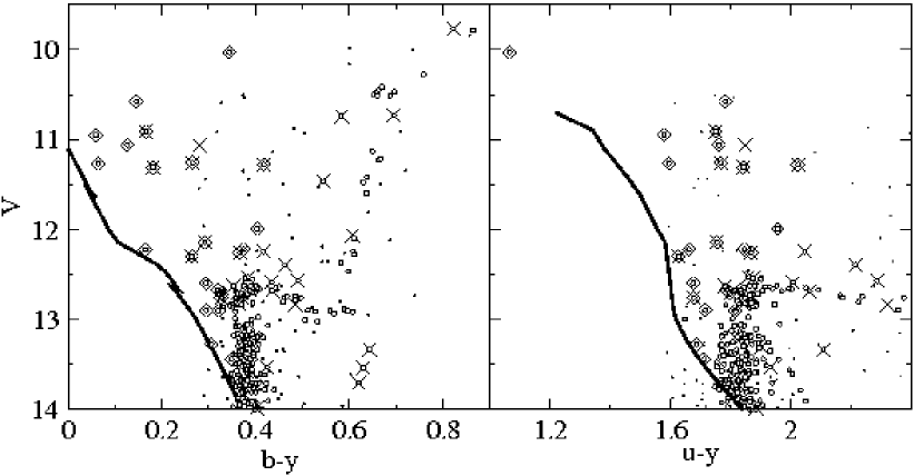
Figure 11: Multiple star systems (marked as crosses) and blue stragglers (diamonds) in a colour magnitude diagram in $b-y$ (left panel) and $u-y$ (right panel) of M 67. Empty circles are candidate member stars. Dots are non-member stars. A ZAMS is shown as reference.

Table 10: The cross-identification of known multiple star systems and their astrometric segregation from this work (last column). First column is our identification number (Table 3), second column that from BDA and third that from Sanders (1977).

ID3	IDBDA	IDS	$b-y$	$V$	$m_{1}$	$c_{1}$	$H_{\beta}$	M/NM
609	22	821	0.371$\pm$0.001	12.764$\pm$0.003	0.150$\pm$0.002	0.436$\pm$0.003		M
629	24	760	0.375$\pm$0.001	13.307$\pm$0.003	0.180$\pm$0.002	0.418$\pm$0.004	2.683$\pm$0.041	M
761	55	752	0.181$\pm$0.001	11.310$\pm$0.003	0.230$\pm$0.002	0.841$\pm$0.004	2.735$\pm$0.006	M
777	61	757	0.425$\pm$0.004	13.530$\pm$0.003	0.124$\pm$0.006	0.410$\pm$0.008	2.640$\pm$0.000	M
806	65	1077	0.435$\pm$0.002	12.587$\pm$0.003	0.173$\pm$0.003	0.358$\pm$0.004	2.638$\pm$0.005
905	86	1063	0.630$\pm$0.001	13.538$\pm$0.003	0.377$\pm$0.002	0.244$\pm$0.004	2.575$\pm$0.008	M
910	88	1053	0.417$\pm$0.001	12.245$\pm$0.003	0.211$\pm$0.002	0.375$\pm$0.004	2.605$\pm$0.008	M
924	90	975	0.281$\pm$0.001	11.063$\pm$0.003	0.166$\pm$0.002	0.676$\pm$0.004	2.666$\pm$0.011	NM
962	102	2206	0.463$\pm$0.001	12.396$\pm$0.003	0.241$\pm$0.002	0.346$\pm$0.004	2.607$\pm$0.014	M
992	111	986	0.366$\pm$0.001	12.725$\pm$0.003	0.177$\pm$0.002	0.414$\pm$0.003	2.624$\pm$0.010	M
1005	117	999	0.491$\pm$0.001	12.569$\pm$0.003	0.254$\pm$0.002	0.308$\pm$0.003	2.595$\pm$0.003	M
1015	119	1045	0.384$\pm$0.001	12.539$\pm$0.003	0.165$\pm$0.002	0.393$\pm$0.003	2.621$\pm$0.004	M
1029	123	1070	0.403$\pm$0.004	13.985$\pm$0.003	0.167$\pm$0.004	0.343$\pm$0.005	2.601$\pm$0.012	M
1033	124	997	0.292$\pm$0.001	12.143$\pm$0.003	0.172$\pm$0.002	0.536$\pm$0.004	2.646$\pm$0.005	M
1046	131	1082	0.266$\pm$0.003	11.260$\pm$0.003	0.120$\pm$0.006	0.731$\pm$0.008	2.704$\pm$0.007	M
1050	134	984	0.367$\pm$0.001	12.259$\pm$0.003	0.180$\pm$0.002	0.409$\pm$0.004	2.626$\pm$0.000	M
1060	136	1072	0.418$\pm$0.001	11.279$\pm$0.003	0.160$\pm$0.002	0.452$\pm$0.004	2.629$\pm$0.007	M
1101	143	1040	0.545$\pm$0.001	11.466$\pm$0.003	0.319$\pm$0.002	0.330$\pm$0.003	2.531$\pm$0.037	M
1102	144	1000	0.484$\pm$0.001	12.836$\pm$0.003	0.253$\pm$0.002	0.364$\pm$0.004	2.596$\pm$0.002	NM
1176	161	1036	0.327$\pm$0.004	12.760$\pm$0.004	0.159$\pm$0.005	0.380$\pm$0.008	2.660$\pm$0.006	M
1206	170	1250	0.823$\pm$0.012	9.769$\pm$0.009	0.555$\pm$0.012	0.372$\pm$0.009	2.593$\pm$0.009	M
1223	173	1264	0.608$\pm$0.001	12.063$\pm$0.003	0.428$\pm$0.002	0.337$\pm$0.004	2.589$\pm$0.012	NM
1237	176	1234	0.353$\pm$0.002	12.627$\pm$0.003	0.165$\pm$0.021	0.393$\pm$0.046	2.626$\pm$0.008	M
1300	190	1284	0.166$\pm$0.002	10.912$\pm$0.003	0.173$\pm$0.003	0.908$\pm$0.004	2.776$\pm$0.003	M
1324	195	1242	0.436$\pm$0.002	12.684$\pm$0.003	0.197$\pm$0.003	0.362$\pm$0.004	2.632$\pm$0.025	M
1352	205	1282	0.644$\pm$0.028	13.334$\pm$0.010	-0.086$\pm$0.030	0.350$\pm$0.028	2.460$\pm$0.028	M
1351	207	1195	0.264$\pm$0.001	12.301$\pm$0.003	0.143$\pm$0.003	0.551$\pm$0.004		M
1402	216	1216	0.387$\pm$0.004	12.673$\pm$0.004	0.136$\pm$0.004	0.379$\pm$0.004	2.728$\pm$0.056	M
1412	219	1272	0.385$\pm$0.001	12.530$\pm$0.003	0.163$\pm$0.002	0.380$\pm$0.004	2.679$\pm$0.075	M
1428	224	1221	0.696$\pm$0.001	10.730$\pm$0.003	0.517$\pm$0.003	0.308$\pm$0.004	2.713$\pm$0.005	M
1488	244	1237	0.583$\pm$0.002	10.741$\pm$0.003	0.350$\pm$0.003	0.350$\pm$0.005		M
987	1050	972	0.556$\pm$0.003	15.395$\pm$0.004	0.277$\pm$0.004	0.238$\pm$0.007	2.593$\pm$0.004
1150	3079	-	0.668$\pm$0.003	15.788$\pm$0.003	0.430$\pm$0.005	0.139$\pm$0.008
1567	3116	1508	0.364$\pm$0.005	12.823$\pm$0.004	0.185$\pm$0.006	0.386$\pm$0.007		M
1085	4004	1024	0.362$\pm$0.001	12.706$\pm$0.003	0.170$\pm$0.002	0.373$\pm$0.003	2.624$\pm$0.001	M
1126	5808	1113	0.621$\pm$0.001	13.703$\pm$0.003	0.321$\pm$0.003	0.188$\pm$0.006		M
1095	5748	1019	0.513$\pm$0.001	14.338$\pm$0.003	0.283$\pm$0.002	0.241$\pm$0.004	2.572$\pm$0.015	M
277	7440	440	0.800$\pm$0.002	8.992$\pm$0.003	-0.062$\pm$0.003	0.688$\pm$0.004		NM
524	32	723	0.535$\pm$0.001	15.690$\pm$0.003	0.366$\pm$0.004	0.341$\pm$0.006		M
1670	2134	1601	0.574$\pm$0.009	14.482$\pm$0.007	0.290$\pm$0.011	0.256$\pm$0.015		NM

A list of the multiple star systems compiled by Sandquist (2004) and present in our photometry is shown in Table 10 with our membership segregation, including in the last two rows the recently discovered eclipsing systems by Sandquist (2006). Figure 11 shows the distribution of multiple star systems and blue stragglers in the colour-magnitude diagram.

The stars S757, S1036 (EV Cnc), S1282 (AH Cnc) and ES379 (ET Cnc), are W UMa contact binaries (where “S” refers to Sanders’s 1977 study and “ES” refers to Eggen & Sandage’s 1964 study). W UMa variables are one class of binary star that can produce blue stragglers after angular momentum loss causes the two stars to coalesce.

6.2 Blue Stragglers

Many studies have been done in M 67 and its rich and varied population of binaries and blue stragglers (BS). It has a super-blue straggler (S977), a single star with a mass of $\sim 3$ M_☉, more than twice the cluster turn-off mass. Gilliland et al. (1993) discovered two BSs with low amplitude $\delta$ Scuti pulsations (S1280 and S1282) and evidence of longer period variations in other stars. Sandquist & Shetrone (2003 hereafter SSh03) discuss that S968, S1066 and S1263 could be long period variables. Sandquist et al. (2003) and van den Berg et al. (2001) point that S1082 is part of a triple system with two components being BSs, one in a close binary and the other one, the brightest component, showing some evidence of being a $\delta$ Scuti star. The close binary is an RS CVn system and also an X-ray source. Other BSs detected in X-rays, S997 and S1072, have wide eccentric orbits whose nature is still not understood (van den Berg et al., 2004). Also with an eccentric orbit, S1284 is an X-ray source, too.

We consider BS candidates those stars that, according to our photometry, are located above and to the blue of the main sequence turnoff (Stryker, 1993; Bailyn, 1995), and, at the same time, have not been classified as non-members in our astrometric analysis. Those member stars that are above the main sequence turnoff but slightly to the red are usually also included in the BSs list. Our selection of BSs is then enlarged by the so-called yellow stragglers (YS), astrometric member stars located between the turnoff and the giant branch, excluding those known to be unresolved binaries with feasible standard components (e.g. Portegies Zwart et al. 1997; van den Berg 2001). This allows a re-evaluation of the membership for not all, but a good part of the stars formerly proposed as BS members of M 67. This helps to clean out the list of bona fide BSs in this cluster. We can perform a further check on the reliability of the selection, drawing the $V$ vs $(u-y)$ diagram (see right panel of Figure 11). Since red giants are faint in $UV$, the photometric blends, which mimic BSs in visible colour-magnitude diagrams are less problematic (see for example Sabbi et al. 2004). We find a total of 23 BS candidates, listed in Table 11. Two of them, S489 and S1466, had not been proposed as BSs before. S1466 was considered non-member by some authors (Sanders, 1977; Girard et al., 1989), but it shows X-ray emision as detected by Chandra (van den Berg et al., 2004).

The work by Deng et al. (1999, hereafter DCLC99), based in the extensive photometry by Fan et al. (1996), proposes a list of 24 BSs. Of them, 17 are astrometric members contained in Table 11, and 2 others (S977 and S2226) appear in our BS selection but they are not covered by our astrometric study. BSs S1031 and S1440 are not included in DCLC99’s list, but they had been also considered as BSs by Ahumada & Lapasset (1995) and SSh03.

The list by DCLC99 includes five stars not in Table 11. The reason is that one of them (S975) has an astrometry incompatible with being a member, two other (S1267 and S1434) are astrometric members but are not covered by our photometry, and the other two (S145 and S277) are neither in our astrometric nor photometric studies.

Other stars (S740, S821, S856 S1165, S1183) proposed as BSs by Ahumada & Lapasset (1995) are already considered normal turnoff member stars by SSh03 and DCLC99, a conclusion supported by our results. S1947, also proposed by Ahumada & Lapasset (1995), is not covered by our studies.

The BS population of M 67 is believed to be abnormally large with respect to other open clusters. Ahumada & Lapasset (1995) give a ratio of the number of BSs to that of main-sequence stars within 2 magnitudes below the turnoff, $N_{\rm BS}/N_{2}$, of 30/200 for this cluster, with a mean of 0.025 for clusters with 6.5 $<\log t<$ 8.6. However, we find in our sample a ratio of $N_{\rm BS}/N_{2}$ = 23/289, similar to the 24/286 found by DCLC99, in closer agreement with the average found among other open clusters.

Table 11: Our BS candidates in M 67, and their photometry. First column is our identification number (Table 3), second column that from BDA, and third that from Sanders (1977). Last column gives the astrometric membership (void values for stars without astrometric membership determination).

ID3	IDBDA	IDS	$b-y$	$V$	$m_{1}$	$c_{1}$	$H_{\beta}$	M/NM
559	16	751	0.330$\pm$0.001	12.700$\pm$0.003	0.172$\pm$0.002	0.464$\pm$ 0.004	2.914$\pm$0.029	M
761	55	752	0.181$\pm$0.001	11.310$\pm$0.003	0.230$\pm$0.002	0.841$\pm$ 0.004	2.735$\pm$0.006	M
883	81	977	0.344$\pm$0.004	10.032$\pm$0.003	0.016$\pm$0.005	0.003$\pm$ 0.026	2.706$\pm$0.005
947	95	1005	0.319$\pm$0.001	12.673$\pm$0.003	0.191$\pm$0.002	0.450$\pm$ 0.003	2.637$\pm$0.006	M
1033	124	997	0.292$\pm$0.001	12.143$\pm$0.003	0.172$\pm$0.002	0.536$\pm$ 0.004	2.646$\pm$0.005	M
1042	130	2204	0.295$\pm$0.001	12.898$\pm$0.003	0.168$\pm$0.002	0.496$\pm$ 0.004	2.671$\pm$0.004	M
1046	131	1082	0.266$\pm$0.003	11.260$\pm$0.003	0.120$\pm$0.006	0.731$\pm$ 0.008	2.704$\pm$0.007	M
1050	134	984	0.367$\pm$0.001	12.259$\pm$0.003	0.180$\pm$0.002	0.409$\pm$ 0.004	2.626$\pm$0.000	M
1060	136	1072	0.418$\pm$0.001	11.279$\pm$0.003	0.160$\pm$0.002	0.452$\pm$ 0.004	2.629$\pm$0.007	M
1140	153	968	0.064$\pm$0.001	11.267$\pm$0.003	0.209$\pm$0.002	0.987$\pm$ 0.004	2.803$\pm$0.008	M
1154	156	1066	0.059$\pm$0.001	10.948$\pm$0.003	0.203$\pm$0.003	0.997$\pm$ 0.004	2.847$\pm$0.003	M
1176	161	1036	0.327$\pm$0.004	12.760$\pm$0.004	0.159$\pm$0.005	0.380$\pm$ 0.008	2.660$\pm$0.006	M
1272	184	1280	0.165$\pm$0.001	12.223$\pm$0.003	0.174$\pm$0.002	0.820$\pm$ 0.004	2.779$\pm$0.011	M
1274	185	1263	0.126$\pm$0.001	11.062$\pm$0.003	0.218$\pm$0.002	0.949$\pm$ 0.004	2.639$\pm$0.012	M
1300	190	1284	0.166$\pm$0.002	10.912$\pm$0.003	0.173$\pm$0.003	0.908$\pm$ 0.004	2.776$\pm$0.003	M
1351	207	1195	0.264$\pm$0.001	12.301$\pm$0.003	0.143$\pm$0.003	0.551$\pm$ 0.004		M
1370	210	1273	0.375$\pm$0.001	12.220$\pm$0.003	0.160$\pm$0.002	0.403$\pm$ 0.003	2.641$\pm$0.011	M
1649	282	1440	0.349$\pm$0.005	13.441$\pm$0.005	0.112$\pm$0.007	0.442$\pm$ 0.007		M
1087	4006	1031	0.306$\pm$0.001	13.277$\pm$0.003	0.171$\pm$0.002	0.428$\pm$ 0.003	2.648$\pm$0.008	M
1181	9226	2226	0.294$\pm$0.004	12.596$\pm$0.004	0.139$\pm$0.005	0.517$\pm$ 0.006
1529	261	1466	0.146$\pm$0.002	10.577$\pm$0.003	0.275$\pm$0.003	0.796$\pm$ 0.004		M
261	7489	489	0.321$\pm$0.002	12.903$\pm$0.003	0.187$\pm$0.003	0.478$\pm$ 0.004		M
659	30	792	0.403$\pm$0.002	11.993$\pm$0.003	0.132$\pm$0.003	0.485$\pm$ 0.004	2.732$\pm$0.014	M

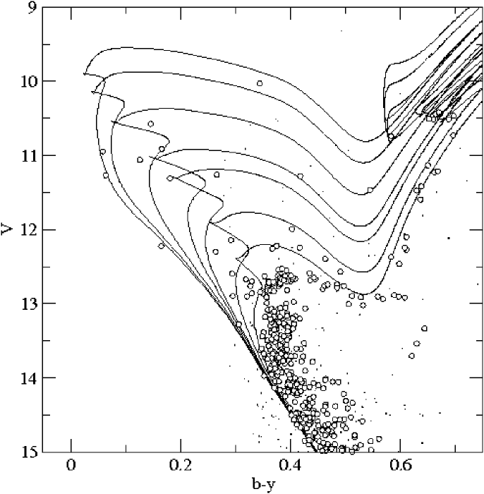
Figure 12: Isochrones from Pietrinferni et al. 2004 from left to right: and 2.5, 1.8, 1.2, 1.0, 0.7, 0.5, 0.4 Gyr for M 67.

We can derive photometric estimates of BS masses by comparing their position in the colour-magnitude diagram with the appropriate isochrones (see Figure 12) from the set of Pietrinferni et al. (2004) with the corresponding metallicities, reddening and distance modulus. We have plotted the standard isochrones from 2.5 Gyr ($M_{\rm TO}$ = 1.46 M_☉), 1.8, 1.2, 1.0, 0.7, 0.5 and 0.4 Gyr ($M_{\rm TO}$ = 2.70 M_☉). The reported isochrones encompass the whole distribution of BSs, thus constraining the range of masses covered to 1.5 M${}_{\sun}\leq M_{\rm BS}\leq$ 2.7 M_☉ for M 67. BSs with $M_{\rm BS}\leq$ 1.5 M_☉, i.e. formed by the merging of low mass main-sequence stars, are still hidden in the main sequence. There are some BSs that cannot lie on the main sequence of any reasonable isochrone, but which can be well fit by the sub-giant branch sequences. These stars, mentioned above, have evolved to the thinning hydrogen burning shell phase and are rapidly moving to the base of the RGB, i.e., they are YS, and also some of these are candidates to be evolved blue stragglers (E-BS), i.e, a BS in its helium-burning phase (see Bellazzini et al. 2002 and references therein).

6.3 Anomalous clump in the colour-magnitude diagram

The presence of a striking clump of stars around $V\sim$ 16, $b-y\sim$ 0.4, $v-y\sim$ 1.1, can be noticed in Fig. 7. This accumulation of stars in the same area cannot be casual and deserves further consideration. We have dubbed this group Lola’s Bunch, after one of the authors of this paper. There are approximately 60 stars in this clump on the $V$ vs $b-y$ diagram, where this accumulation reaches a density more than twice that of the surrounding areas of the photometric space. Furthermore, the spatial distribution of the stars (Fig. 13) shows a lack of them in the centre of the cluster. The average distance from the centre of these stars is $r$ =19.94$\pm$7.85$\arcmin$.

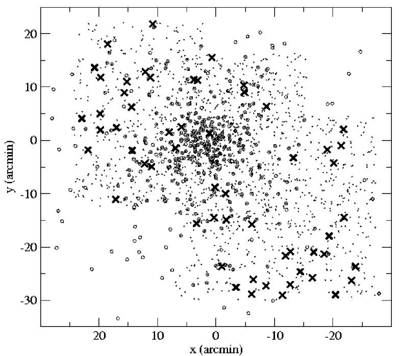
Figure 13: Spatial distribution of clump stars (crosses) and members from our astrometric study (empty circles) in M 67 area. Dots represent the stars present in our CCD photometric sample: their spatial coverage does not reach the lower right nor the upper left corners. Clump stars, selected exclusively on a photometric basis, are disposed around the cluster centre, at an average distance of 20$\arcmin$ and leaving a void in the middle. North is up, East is left.

We have looked for photometry of different sources to check the reality of the bunch, discarding any bizarre photometric effect in our data. We have seen that the only existing study covering an area wide enough to include the stars that induce this feature is the one by Fan et al. (1996) using the BATC system, that covers almost two square degrees.

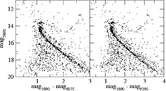
Figure 14: The BATC colour-colour diagrams in the central 50$\times$50$\arcmin$ area of M 67. The BATC filters are marked by their wavelenghts.

In Fig. 14 we can see a colour-magnitude diagram of the central 50$\arcmin\times$50$\arcmin$ area of M 67 in two different colours: mag3890 vs 3890-6075 and 3890-9190. Although the contrast is lower than the factor two found in the Strömgren passbands, the bunch also appears as a significant accumulation in the diagrams, with a local density equal to 1.5 times that of the surronding area in the colour-magnitude diagram mag3890 vs 3890-9190, and 1.75 times in the colour-magnitude diagram mag3890 vs 3890-6075. It is worth noting that the bunch is more noticeable when using the BATC filter 3890, quite similar to Strömgren $v$. The lack of clump members at the central region of the cluster is also observed in BATC data.

Stars placed in this photometric region of the colour-magnitude diagram are found all over the two square degrees field covered by BATC data, but we have noticed that the bunch gives a better constrast when selecting the central 50$\arcmin\times$50$\arcmin$. This is also approximately the area covered by our Strömgren photometry, and coincides with the spatial area over which most astrometric members are concentrated (Fig. 5).

Considering the main observational facts, we see that any of the two possible options (clump stars being members or non-members) places ourselves in front of an interesting finding. If those stars were mainly cluster members, then their photometry could be explained if they were detached binaries composed by a white dwarf and a red dwarf, i.e: pre-cataclysmic variable stars (pre-CVs). Current knowledge of white dwarfs and pre-CV stars indicates that the combinations required to obtain the observed colours are physically feasible (Bergeron et al. 1995). Stassun et al. (2002) have found that five stars in this photometric area of M 67 colour-magnitude diagram are variables of kinds compatible with the pre-CV status, but they failed to perceive the relevance of this concentration of stars in their data. Confirming the existence of a significant population of pre-CV stars in such a well studied open cluster (and thus, of known distance, age and metallicity) would have very deep implications for the understanding of the nature and evolution of these binary systems. First, their clumping in a region of the colour-magnitude diagram, and not on a locus following the trend that would be expected from the white dwarf cooling sequence, would impose tight restrictions to the evolutionary history of the precursor binary systems. Second, their distribution in the outer region of the cluster could only be explained in terms of mass segregation, implying that the pairs have had enough time to experience this dynamical process since the mass-loss that made them as light as they would be now.

The other option, having a clump made up from field stars, is no less challenging. The relatively narrow intervals of apparent magnitude and colour means that all these stars have similar spectral type and, thus, similar absolute magnitude and distance. In this case, we would have to explain how could be formed an accumulation of field G stars, at a definite distance: we would have a curtain or stream of G stars placed twice as far as M 67. Furthermore, their spatial distribution (that seemingly avoids the centre of M 67) would require some explanation.

The scarcity of the data available make any further consideration to lay into the realm of speculation: we have already started spectroscopic observations with the aim of clarifying the nature of this peculiar bunch of stars.

7 Conclusions

In this paper we give a catalogue of accurate Strömgren $uvby-H_{\beta}$ and J2000 coordinates for 1843 stars in an area of 50${\arcmin}$$\times$50${\arcmin}$ around M 67. We give a selection of probable members of M 67 combining this photometric study with astrometric analysis using parametric as well as non-parametric approaches. A better determination of this cluster physical parameters based on our accurate photometry gives: $E(b-y)$ = 0.03$\pm$0.03, [Fe/H] = 0.01$\pm$0.14, a distance modulus of $V_{0}-M_{V}$ = 9.7$\pm$0.2 and an age of 4.2$\pm$0.2 Gyr ($\log t$=9.6$\pm$0.1). The values are coherent with previous studies (see Chen et al. (2003) and references therein).

An anomalous bunch of more than 60 stars in the colour-magnitude diagram around $V$ = 16, (b-y) = 0.4 is tentatively interpreted as composed of pre-CVs belonging to the cluster, or as a stream of G stars placed twice as far as the cluster, two alternatives to be tested with further observations.