A High-Throughput Cross-Layer Scheme for Distributed Wireless Ad Hoc Networks

Abstract

In wireless ad hoc networks, distributed nodes can collaboratively form an antenna array for long-distance communications to achieve high energy efficiency. In recent work, Ochiai, et al., have shown that such collaborative beamforming can achieve a statistically nice beampattern with a narrow main lobe and low side lobes. However, the process of collaboration introduces significant delay, since all collaborating nodes need access to the same information. In this paper, a technique that significantly reduces the collaboration overhead is proposed. It consists of two phases. In the first phase, nodes transmit locally in a random access fashion. Collisions, when they occur, are viewed as linear mixtures of the collided packets. In the second phase, a set of cooperating nodes acts as a distributed antenna system and beamform the received analog waveform to one or more faraway destinations. This step requires multiplication of the received analog waveform by a complex number, which is independently computed by each cooperating node, and which enables separation of the collided packets based on their final destination. The scheme requires that each node has global knowledge of the network coordinates. The proposed scheme can achieve high throughput, which in certain cases exceeds one.

Keywords: distributed wireless systems, cooperation, beamforming

I Introduction

Energy is often a scarce commodity in wireless sensor networks, as wireless sensors typically operate on batteries, which in many cases are hard to replace. Similarly, due to cost consideration, nodes in wireless ad hoc sensor networks are commonly equipped with only a single omnidirectional antenna. Thus, in order to transmit information over long distances while conserving energy and maintaining a certain transmission power threshold, multihop networks have been the preferred solution. However, there are several challenges in transmitting real-time services over multiple hops. For example, the traditional CSMA/CA based media access control for avoiding collisions does not work well in a multihop scenario because transmitters are often out of reach of other users’ sensing range. Thus, as packets travel across the network, they experience interference and a large number of collisions, which introduces delays. Also, multihop networks require a high node density which makes routing more difficult and affects the reliability of links [1].

Recently, a collaborative beamforming technique was proposed in [3], in which randomly distributed nodes in a network cluster form an antenna array and beamform data to a faraway destination without each node exceeding its power constraint. The destination receives data with high signal power. Beamforming with antenna arrays is a well studied technology; it provides space-division multiple access (SDMA) which enables significant communication rate increase. The main challenge with implementing beamforming based on randomly distributed nodes in the network is that the geometry of the network changes dynamically. It was shown in [3] that such a distributed antenna array can achieve a nice average beampattern with a narrow main lobe and low side lobes. The directivity of the pattern increases as the number of collaborating nodes increases. Such an approach, when applied in the context of a multihop network reduces the number of hops needed, thereby reducing packet delays and improving throughput. However, one must take into account the overhead required for node collaboration, i.e., sharing of the information to be transmitted jointly by the nodes. If a time-division multiple-access (TDMA) scheme were to be employed, the information-sharing time would increase proportionally to the number of nodes involved in the collaboration.

In this paper we present a technique based on the idea of collaborative beamforming, that reduces the time required for information sharing. The technique also allows different nodes in the network to transmit simultaneously. Collaborating nodes receive linear mixtures of the transmitted packets. Subsequently, each collaborating node transmits a weighted version of its received signal. The weights are such that one or multiple beams are formed, each focusing on one destination node, and reinforcing the signal intended for a particular destination as compared to the other signals. Each collaborating node computes its weight based on the channel coefficients between sources and itself, estimated by orthogonal node IDs embedded in the packets. The proposed scheme achieves higher throughput and lower delay with the cost of lower SINR as compared to [3].

II Background on collaborative beamforming

For simplicity, let us assume that the sources and destinations are coplanar. We index source nodes using a subscript $i,$ with $t_{i}$ denoting the $i$-th node. The locations of these nodes follow a uniform distribution over a disk of radius $R,$ and it is assumed that each node knows its own location. We denote the location of $t_{i}$ in polar coordinates with respect to the center of the disk by $(r_{i},\psi_{i}).$

Suppose that a set of $N$ nodes designated as collaborating nodes have access to the same signal, i.e., $s(n)$, whose destination is at azimuthal angle $\phi_{0}$. Let $d_{i}(\phi_{0})$ denote the distance between the $i$-th collaborating node and the destination. The initial phases at the collaborating nodes are set to

$$\Psi_{i}(\phi_{0})=-\frac{2\pi}{\lambda}d_{i}(\phi_{0}),\ i=1,...,N$$ (1)

which requires knowledge of distances relative to wavelength between nodes and destination, and applies to the closed-loop case [3]. Alternatively, the initial phase of node $i$ could be:

$$\Psi_{i}(\phi_{0})=\frac{2\pi}{\lambda}r_{i}\cos(\phi_{0}-\psi_{i})$$ (2)

which requires knowledge of the node’s position relative to some common reference point, and corresponds to the open-loop case [3]. In both cases synchronization is needed, which can be achieved via the use of the Global Positioning System (GPS).

The channels between collaborating nodes and destination are assumed to be idential for all nodes. The corresponding array factor given the collaborating nodes at radial coordinates ${\mathbf{r}}=[r_{1},...,r_{N}]$ and azimuthal coordinates ${\bm{\psi}}=[\psi_{1},...,\psi_{N}]$ is

$$F(\phi|{\bf r,\bm{\psi}}) = \frac{1}{N}\sum_{i=1}^{N}e^{j\Psi_{i}(\phi_{0})}e^{j\frac{2\pi}{\lambda}d_{i}(\phi)}$$ (3)

Under far-field assumptions, the array factor becomes [3]:

$$F(\phi|{\bf r,\bm{\psi}}) = \frac{1}{N}\sum_{i=1}^{N}e^{j\alpha(\phi;\phi_{0})z_{i}}$$ (4)

where $\alpha(\phi;\phi_{0})=4\pi\tilde{R}\sin(\frac{1}{2}(\phi_{0}-\phi))$, $\tilde{R}=R/\lambda$ and $z_{i}=(r_{i}/R)\sin(\psi_{i}-\frac{1}{2}(\phi_{0}+\phi))$ with the following pdf:

$$f_{z_{i}}(z)=\frac{2}{\pi}\sqrt{1-z^{2}}, \ -1\leq z\leq 1$$ (5)

Finally, the average beampattern can be expressed as [3]

$$P_{\mathrm{av}}(\phi) = E_{z}\{|F(\phi|{\bf z})|^{2}\}$$ (6)

$$= \frac{1}{N}+\left(1-\frac{1}{N}\right)\left|2\frac{J_{1}(\alpha(\phi;\phi_{0}))}{\alpha(\phi;\phi_{0})}\right|^{2}$$

where $J_{1}(.)$ is the first-order Bessel function of the first kind. When plotted as a function of $\phi$, $P_{\mathrm{av}}(\phi)$ exhibits a main lobe around $\phi_{0}$, and side lobes away from $\phi_{0}$. It equals one in the target direction, and the sidelobe level approaches $1/N$ as the angle moves away from the target direction. The statistical properties of the beampattern were analyzed in [3], where it was shown that under ideal channel and system assumptions, directivity of order $N$ can be achieved asymptotically with $N$ sparsely distributed sensors.

As we have noted, all of the collaborating nodes must have the same information to implement beamforming. Thus, the active nodes need to share their information symbols with all collaborating nodes in advance. If a time-division multiple-access (TDMA) scheme were to be employed, the information-sharing time would increase proportionally to the number of active nodes. In the following, we propose a novel scheme to reduce the information-sharing time and also allow nodes in the network to transmit simultaneously.

III The proposed scheme

Here we refine the model of [3], focusing more directly on the physical models for the signal, fading channel and noise. Besides the assumptions in Section II, we will further assume the followings:

(1) The network is divided into clusters, so that nodes in a cluster can hear each other. In each cluster there is a node designated as the cluster-head (CH). Nodes in a cluster do not need to transmit their packets through the CH.

(2) A slotted packet system is considered, in which each packet requires one slot for its transmission. Perfect synchronization is assumed between nodes in the same cluster.

(3) Nodes operate under half-duplex mode, i.e., they cannot receive while they are transmitting.

(4) Nodes transmit packets consisting of PSK symbols having the same variance $\sigma_{s}^{2}$. Each transmitted packet contains (in fixed locations) a set of pilots comprising the user ID, followed by a set of pilots comprising the destination information.

(5) Communication takes place over flat fading channels. The channel gain during slot $n$ between source $t_{i}$ and collaborating node $c_{j}$ is denoted by $a_{ij}(n)$. It does not change within one slot, but can change between slots. The gains $a_{ij}$ follows a Rayleigh fading model, being i.i.d. complex Gaussian random variables with zero means and variances $\sigma_{a}^{2}$.

(6) The complex baseband-equivalent channel gain between nodes $c_{i},d_{j}$ is [4]: $b_{ij}=b\cdot e^{{j\frac{2\pi r_{ij}}{\lambda}}}$ where $r_{ij}$ is the distance between nodes $c_{i},d_{j},$ and where $b$ is the path loss. The distances between collaborating nodes and destinations are much greater than distances between source and collaborating nodes. Thus, $b$ is assumed to be identical for all collaborating nodes and equals the path loss between the origin of the disk over which the nodes are distributed to the destination.

(7) the noise vectors are uncorrelated, complex, zero-mean white Gaussian vectors.

Suppose that cluster $C$ contain $J$ nodes. At slot $n$, nodes $t_{1},\ldots,t_{K}$ need to communicate with node $d_{1},\ldots,d_{K}$ that belong to cluster $C_{1},\ldots,C_{K}$, respectively. The azimuthal angle of destination $d_{i}$ is denoted by $\phi_{i}$. The packet transmitted by $t_{j}$ consists of $M$ symbols $\mathbf{s}_{j}(n)\triangleq[s_{j}(n;0),\ldots,s_{j}(n;M-1)]$. Due to the broadcast nature of the wireless channel, non-active nodes in cluster $C$ hear a collision, i.e., a linear combination of the transmitted symbols. More specifically, node $c_{i}$ hears the signal

$$\mathbf{x}_{i}(n)=\sum_{j=1}^{K}a_{ji}(n)\mathbf{s}_{j}(n)+\mathbf{w}_{i}(n)$$ (7)

where $\mathbf{w}_{i}(n)=[w_{i}(n;0),\ldots,w_{i}(n;M-1)]$ is noise vector with variance $\sigma_{w}^{2}$ at the receiving node $c_{i}$.

Once the CH establishes that there has been a transmission, it initiates a collaborative transmission period (CTP), by sending to all nodes a control bit, e.g., $1$, via an error-free control channel. The CH will continue sending a $1$ in the beginning of each subsequent slot until the CTP has been completed. The cluster nodes cannot transmit new packets until the CTP is over.

Suppose that each transmitted packet includes an ID sequence, so that IDs are orthogonal between different users. The channel coefficients can be estimated by cross correlating $\mathbf{x}_{i}(n)$ with known user IDs as in [2]. If the magnitude of the cross-correlation in greater than some threshold, then the corresponding user is in the mixture, and the value of the cross-correlation provides the corresponding channel coefficient. The information of destination nodes could be obtained in a similar way.

Each node $c_{i}$ uses cross-correlation operations with known orthogonal user IDs to determine which users are in the mixture, the corresponding destinations, and also the coefficients $a_{ij}$.

Let $d_{m}$ denote the destination of $\mathbf{s}_{m}(n)$. In slot $n+m,\ m=1,\ldots,K$, each collaborating node $c_{i}$ transmits the signal:

$$\tilde{\mathbf{x}}_{i}(n+m)=\mathbf{x}_{i}(n)\mu_{m}a^{*}_{mi}(n)e^{-j\frac{2\pi}{\lambda}d_{i}(\phi_{m})}$$ (8)

where $d_{i}(\phi_{m})$ denotes the distance between user $i$ and destination node $d_{m}$ with azimuth $\phi_{m}$, and $\mu_{m}$ is a scalar to adjust transmit power and same for all collaborating nodes. In addition, $\mu_{m}$ is of the order of $1/N$.

Given the collaborating nodes at radial coordinates ${\mathbf{r}}=[r_{1},...,r_{N}]$, azimuthal coordinates ${\bm{\psi}}=[\psi_{1},...,\psi_{N}]$ and the path loss $b$, the received signal at direction $\phi$ is:

$$\mathbf{y}(\phi;m|{\mathbf{r},\bm{\psi}})=\sum_{i=1}^{N}b\tilde{\mathbf{x}}_{i}(n+m)e^{j\frac{2\pi}{\lambda}d_{i}(\phi)}+\mathbf{v}(n+m)$$ (9)

where $\mathbf{v}(n+m)$ is the noise vector with variance $\sigma_{v}^{2}$ at the receiver during slot $n+m$.

Let us consider the received signal at the destination $d_{m}$ at angle $\phi_{m}$ during slot $n+m$:

$$\mathbf{y}(\phi_{m};m) = \sum_{i=1}^{N}b\tilde{\mathbf{x}}_{i}(n+m)+\mathbf{v}_{m}(n+m)$$ (10)

$$= \mu_{m}b\sum_{i=1}^{N}[|a_{mi}(n)|^{2}\mathbf{s}_{m}(n)+a^{*}_{mi}(n)\mathbf{w}_{i}(n)$$

$$+a^{*}_{mi}(n)\sum_{j=1\ \atop j\neq m}^{K}a_{ji}(n)\mathbf{s}_{j}(n)]+\mathbf{v}_{m}(n+m)$$

As $N\rightarrow\infty$, $\frac{1}{N}\sum_{i=1}^{N}|a_{mi}(n)|^{2}\rightarrow E\{|a_{mi}|^{2}\}=\sigma_{a}^{2}$. Also, $\frac{1}{N}\sum_{i=1}^{N}\ a^{*}_{mi}(n)a_{ji}(n)\rightarrow E\{a_{mi}^{*}a_{ji}\}=0$, due to the fact that for $j\neq m$, the channel coefficients $a_{mi},a_{ji}$ are uncorrelated and have zero mean. Finally, as $N\rightarrow\infty$ and omitting the noise, $\mathbf{y}(\phi_{m};m|{\bf r,\bm{\psi}})\rightarrow N\mu_{m}b_{m}\sigma_{a}^{2}\mathbf{s}_{m}(n)$. Thus, the destination node $d_{m}$ receives a scaled version of $\mathbf{s}_{m}(n)$. The beamforming step is completed in $K$ slots, reinforcing one source signal at a time.

Assuming that all of the $K$ source packets have distinct destinations at different resolvable directions, multiple beams can be formed in one slot, each beam focusing on one direction and reinforcing one source signal. The transmitted signal from each collaborating node would be:

$$\tilde{\mathbf{x}}_{i}(n+1)=\mathbf{x}_{i}(n)\sum_{m=1}^{K}\mu_{m}a^{*}_{mi}(n)e^{-j\frac{2\pi}{\lambda}d_{i}(\phi_{m})}$$ (11)

The received signal at destinations would then be:

$$\mathbf{y}(\phi|{\mathbf{r},\bm{\psi}})=b\tilde{\mathbf{x}}_{i}(n+1)e^{j\frac{2\pi}{\lambda}d_{i}(\phi)}+\mathbf{v}(n+1)$$ (12)

It can be shown that as $N\rightarrow\infty$ and omitting noise, $\mathbf{y}(\phi_{m}|{\mathbf{r},\bm{\psi}})\rightarrow N\mu_{m}b\sigma_{a}^{2}\mathbf{s}_{m}(n)$, for $m=1,...,K$. Thus, each of the $K$ beams transmits a scaled version of a source signal to its destination. Based on (9), (12), we can easily extend the mathematical formulation to the scenario that not all of the $K$ packets have distinct destinations.

In the rest of the paper, for simplicity we will consider only the case in which a single beam is formed during slot $n+m$, focusing on destination $d_{m}$. The results obtained under this assumption can be readily extended to multiple simultaneous beams. The time index can be omitted without causing confusion. Also, we are particularly interested in the average properties over a statistical ensemble, so the analysis can be based on one sample of a packet assuming samples are independent. Substituting $\mathbf{y}$, $\tilde{\mathbf{x}}$, $\mathbf{x}$, $\mathbf{w}$, $\mathbf{v}$ in (7)-(9) by $y$, $\tilde{x}$, $x$, $w$, $v$ (i.e., with one of their samples) respectively, we get:

$$y(\phi;m|{\mathbf{r},\bm{\psi}})=\sum_{i=1}^{N}b\tilde{x}_{i}e^{j\frac{2\pi}{\lambda}d_{i}(\phi)}+v$$ (13)

IV Performance of the average beampattern

In this section we analyze the average beampattern. Under the far-field assumption, and following the steps in [3], (13) can be expressed as:

$$y(\phi;m|{\mathbf{r},\bm{\psi}})=\sum_{i=1}^{N}\mu_{m}ba_{mi}^{*}e^{-j\alpha(\phi;\phi_{m})z_{i}}(\sum_{j=1}^{K}{a_{ji}s_{j}}+w_{i})+v$$ (14)

where $\alpha(\phi;\phi_{m})$ and $z_{i}$ are the same as those in (4).

The far-field beampattern or the received power is defined as:

$$P(\phi)=|y(\phi;m|{\mathbf{r},\bm{\psi}})|^{2}$$ (15)

Taking into account the assumptions on the channel coefficients, it can be readily shown that the average beampattern equals:

$$P_{\mathrm{av}}(\phi) \triangleq E_{z,a,w,v}\{P(\phi;\phi_{m})\}$$ (16)

$$= \mu_{m}^{2}b^{2}E\{|s_{m}|^{2}\sum_{i=1}^{N}|a_{mi}|^{4}$$

$$+|s_{m}|^{2}\sum_{i=1}^{N}\sum_{\ell=1\atop\ell\neq i}^{N}|a_{mi}|^{2}|a_{m\ell}|^{2}e^{-j\alpha(\phi;\phi_{m})(z_{i}-z_{\ell})}$$

$$+\sum_{j=1\atop j\neq m}^{K}|s_{j}|^{2}\sum_{i=1}^{N}|a_{mi}|^{2}|a_{ji}|^{2}+\sum_{i=1}^{N}{|a_{mi}|^{2}}|w_{i}|^{2}+|v|^{2}\}$$

$$= N\mu_{m}^{2}b^{2}[2\sigma_{s}^{2}\sigma_{a}^{4}+(N-1)\sigma_{s}^{2}\sigma_{a}^{4}E\{e^{-j\alpha(\phi;\phi_{m})(z_{i}-z_{\ell})}\}$$

$$+(K-1)\sigma_{s}^{2}\sigma_{a}^{4}+\sigma_{w}^{2}\sigma_{a}^{2}]+\sigma_{v}^{2}$$

Then,

$$P_{\mathrm{av}}(\phi)=N^{2}\mu_{m}^{2}b^{2}\sigma_{s}^{2}\sigma_{a}^{4}\left(\frac{\beta}{N}+(1-\frac{1}{N})\left|2\cdot\frac{J_{1}(\alpha(\phi;\phi_{m}))}{\alpha(\phi;\phi_{m})}\right|^{2}\right)$$ (17)

where

$$\beta=K+1+\frac{\sigma_{w}^{2}}{\sigma_{s}^{2}\sigma_{a}^{2}}+\frac{N\sigma_{v}^{2}}{\mu_{m}^{2}b^{2}\sigma_{s}^{2}\sigma_{a}^{4}}$$ (18)

The term $N\mu_{m}^{2}b^{2}\sigma_{s}^{2}\sigma_{a}^{4}\beta$ represents the average power of the sidelobes that is independent of the angle $\phi$. Note that (17) is of the similar form with (6). Thus, other properties of the average beampattern like peak/zero positions and 3-dB bandwidth/sidelobe region can be easily obtained based on corresponding results of [3], and are omitted here.

V Performance of the network

V-A Throughput

Suppose that $K$ packets need to be transmitted. For the collaborative beamforming scheme of [3], each packet must be shared by the $N$ beamforming nodes. If one wished to avoid collisions, TDMA would be a natural way to implement information sharing. With the use of TDMA, in each slot one active node is scheduled to broadcast its packet to other nodes within the same cluster. The sharing of information would require $K$ slots. Via the use of multiple beams, the beamforming to the destination would require $1$ slot if destinations are distinct, or up to $K$ slots in the worst case where all nodes have the same destination. Thus, for the scheme of [3], the throughput, $T$ satisfies: $1/2\leq T\leq K/(K+1)$.

In the proposed scheme, combinations of $K$ packets enter the system and reach $N$ collaborating nodes in $1$ slot. Via multiple beams, the packets can be delivered to their destinations in one additional slot, if the destinations are distinct. The throughput is then $K/(1+1)=K/2$. If two or more packets have a common destination, the beamforming will need to take more than one slot. In the worst case where all packets have the same destination, $K$ slots will be needed, resulting in a total throughput of $K/(1+K)$. Thus, $K/(1+K)\leq T_{\mathrm{proposed}}\leq K/2$. Note that the throughput of the proposed scheme could be greater than 1.

V-B Transmit Power and Average SINR

In this section, we analyze the SINR under the same transmit power for the scheme of [3] and the proposed scheme.

Although the focus in [3] was on the statistical properties of the beampattern, we can extend (4)-(6) to a physical model including signal, path loss and noise. The received signal of the destination $d_{m}$ is given by:

$$\overline{y}(\phi;m|{\mathbf{r},\bm{\psi}})=\sum_{i=1}^{N}b\bar{\mu}_{m}s_{m}e^{-j\alpha(\phi;\phi_{m})z_{i}}+v$$ (19)

$c_{i}$ simply transmits $\bar{\mu}_{m}s_{m}e^{-j\frac{2\pi}{\lambda}d_{i}(\phi_{m})}$, and the transmit power is thus $\bar{\mu}_{m}^{2}\sigma_{s}^{2}$. The average beampattern at the target direction $\phi_{m}$ is:

$$\overline{P}_{\mathrm{av}}(\phi_{m})=N^{2}\bar{\mu}_{m}^{2}b^{2}\sigma_{s}^{2}+\sigma_{v}^{2}$$ (20)

and the SINR is

$$\overline{SINR}=\frac{N^{2}\bar{\mu}_{m}^{2}b^{2}\sigma_{s}^{2}}{\sigma_{v}^{2}}$$ (21)

For the proposed scheme, the collaborating node $c_{i}$ transmits $\tilde{x}_{i}$ given by (11). It can be shown the average power of $\tilde{x}_{i}$ equals

$$E\{\tilde{x}_{i}\tilde{x}_{i}^{*}\}=\mu_{m}^{2}\sigma_{s}^{2}\sigma_{a}^{4}\beta^{\prime}$$ (22)

where $\beta^{\prime}=K+1+\frac{\sigma_{w}^{2}}{\sigma_{s}^{2}\sigma_{a}^{2}}$.

To keep the same average transmit power as $\bar{\mu}_{m}^{2}\sigma_{s}^{2}$,

$$\mu_{m}^{2}=\frac{\bar{\mu}_{m}^{2}}{\beta^{\prime}\sigma_{a}^{4}}$$ (23)

Under this value of $\mu_{m}$ and based on (17), the average beampattern at $\phi_{m}$ is given by

$$P_{\mathrm{av}}(\phi_{m}) = \frac{N^{2}\bar{\mu}_{m}^{2}b^{2}\sigma_{s}^{2}}{\beta^{\prime}}\left(1+\frac{\beta^{\prime}-1}{N}\right)+\sigma_{v}^{2}$$ (24)

$$\stackrel{{\scriptstyle n\rightarrow\infty}}{{\longrightarrow}} \frac{N^{2}\bar{\mu}_{m}^{2}b^{2}\sigma_{s}^{2}}{\beta^{\prime}}+\sigma_{v}^{2}\ .$$

Thus, the average received power of the proposed scheme (without the noise term $\sigma_{v}^{2}$) is $\beta^{\prime}$ times less than that of (20). In other words, each collaborating node in the proposed scheme needs to use $\beta^{\prime}$ times more transmit power, in order to (asymptotically) achieve the same average received power as (20).

From (17), (21), (23), (24), the SINR at the destination $d_{m}$ for the proposed scheme is

$$SINR = \frac{(1+\frac{1}{N})N^{2}\mu_{m}^{2}b^{2}\sigma_{s}^{2}\sigma_{a}^{4}}{\frac{\beta^{\prime}-2}{N}N^{2}\mu_{m}^{2}b^{2}\sigma_{s}^{2}\sigma_{a}^{4}+\sigma_{v}^{2}}$$ (25)

$$= \frac{(1+\frac{1}{N})\overline{SINR}}{\frac{\beta^{\prime}-2}{N}\overline{SINR}+\beta^{\prime}}\stackrel{{\scriptstyle n\rightarrow\infty}}{{\longrightarrow}}\frac{\overline{SINR}}{\beta^{\prime}}$$

Thus, compared with (21), the average SINR of the proposed scheme at the destination is still asymptotically scaled down by $\beta^{\prime}$.

VI Simulations

VI-A simulation setup

We investigate the performance of the above scheme for different numbers of collaborating nodes, i.e. $N$. For convenience, and without loss of generality, we divide the nodes in a cluster into two pools: one contains all potential active nodes, the total number of which is fixed $\hat{J}$ = 32 and another contains $N$ collaborating nodes. The directions of destinations are uniformly distributed in $[0,2\pi)$. The locations of collaborating nodes are uniformly distributed within a disk with $\tilde{R}=10$ (i.e., the radius normalized by the wavelength). The channels among nodes in a cluster are selected from zero-mean complex Gaussian processes, which are constant within one slot, but vary between slots.

VI-B BER performance

In the proposed scheme, noise enters the collaborating nodes, with variance $\sigma_{w}^{2}$, and the destination, with variance $\sigma_{v}^{2}$. Let us define $\gamma_{1}\triangleq\sigma_{s}^{2}\sigma_{a}^{2}/\sigma_{w}^{2},$ which represents the average SNR in the process of information sharing, and define $\gamma_{2}\triangleq N^{2}\mu_{m}^{2}b^{2}\sigma_{s}^{2}\sigma_{a}^{4}/\sigma_{v}^{2}$. Note that $\gamma_{2}$ is also independent of $N$ since $\mu_{m}$ is of the order of $1/N$. The overall SINR in (25) can be rewritten by

$$SINR = \frac{1+\frac{1}{N}}{\frac{K-1+\gamma_{1}^{-1}}{N}+\gamma_{2}^{-1}}$$ (26)

which is determined by $\gamma_{1}$, $\gamma_{2}$, $K$ and $N$.

We fix $\gamma_{1}$ to 20 dB to investigate the performance of bit error rate (BER) for different values of $\gamma_{2}$ and $N$. We perform a Monte-Carlo experiment consisting of $10^{6}$ repeated independent trials. Each packet contains BPSK symbols and $K=4$ nodes are transmitting all the time. Fig. 1(a) shows the BER vs. $\gamma_{2}$ for the case in which only one beampattern is formed in each slot, for different values of $N$. Solid lines correspond to estimated channels, number of active nodes and destination information. One can see that BER decreases as $\gamma_{2}$ and $N$ increase. Dashed lines correspond to perfect knowledge of channels, number of active nodes and destination information, and can be considered as lower bounds of BER performance. Fig. 1(b) shows the BER performance in which all of four simultaneous beams are always formed in one slot. Compared with Fig. 1(a), more collaborating nodes are needed to achieve the same BER level.

VI-C Throughput Performance

To investigate performance under certain traffic load $p$, we perform a random experiment consisting of 1,000 repeated independent trials. In each trial, all users are statistically the same, and each user sends out packets with probability $p/\hat{J}$. The throughput is defined as the average number of packets that were successfully transmitted in a time slot. Each packet contains 424 bits with QPSK symbols. The nodes’ ID sequences are selected based on a $\hat{J}$th order Hadamard matrix and the IDs are used to determine the active nodes involved in collisions as well as to estimate the channels. A maximum likelihood decoder is used at the destination nodes to recover the symbols. Packets received at the destinations with BER higher than 0.02 are considered to be lost or corrupted. $\gamma_{1}=\gamma_{2}=20$ dB.

In Figs. 2 (a)-(c), we show the throughput performance for different values of $p$ and $N$, allowing up to 1, 2, 3 simultaneous beampatterns per slot, respectively. The curves with legend “ideal” correspond to the case where all the transmitted packets are successfully received, which can be considered to be an upper bound on the proposed scheme. One can see that the increase of $N$ can result in throughput improvement. Furthermore, for small $N$, one should choose a small number of simultaneous beampatterns to improve throughput. Fig. 2(d) shows the throughput in which all the $K$ beampatterns are allowed to be formed in one slot. Note that $N=1,024$ enables throughput of almost $K/2$.

VII Conclusions and Future work

In this paper we have proposed a technique for reducing the time needed for information sharing during collaborative beamforming, and for allowing simultaneous transmissions. The proposed scheme can achieve high throughput at the cost of reduced SINR. An analysis for the average beampattern and network performance has also been provided. Our analysis is based on a number of ideal assumptions on the system. In future work, we plan to investigate the effects of imperfect channel/phase and non-identical path loss, and also to seek closed-form BER expressions.

(a) one beam per slot

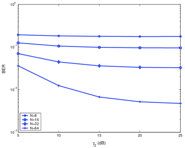
(b) 4 simultaneous beams per slot

Figure 1: BER performance under different $\gamma_{2}$ and $N$ ($K=4$)

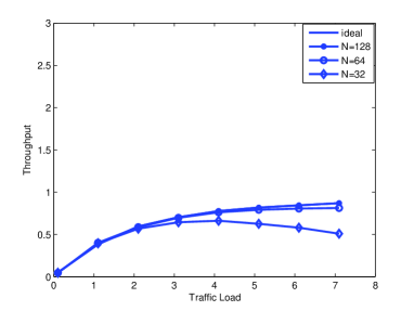
(a) up to one beam per slot

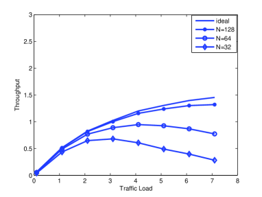
(b) up to two beams per slot

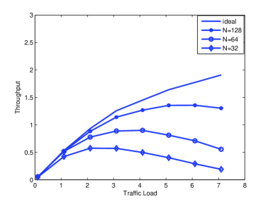
(c) up to three beams per slot

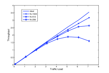
(d) up to $K$ beams per slot

Figure 2: Throughput performance under different traffic load and $N$

References

- [1] H. Gharavi and K. Ban, “Multihop sensor network design for wide-band communications,” Proceedings of the IEEE, Vol. 91, No. 8, pp. 1221 - 1234, Aug. 2003.
- [2] R. Lin and A. P. Petropulu, “New wireless medium access protocol based on cooperation,” IEEE Trans. Signal Process., vol. 53, no 12, pp. 4675 - 4684, Dec. 2005.
- [3] H. Ochiai, P. Mitran, H. V. Poor and V. Tarokh, “Collaborative beamforming for distributed wireless ad hoc sensor networks”, IEEE Trans. Sig. Proc., vol. 53, Issue 11, pp. 4110 - 4124, Nov. 2005.
- [4] D. Tse and P. Viswanath, Fundamentals of Wireless Communication. Cambridge University Press, Cambridge, UK, 2005.