Deterministic characterization of stochastic genetic circuits

Abstract

For cellular biochemical reaction systems where the numbers of molecules is small, significant noise is associated with chemical reaction events. This molecular noise can give rise to behavior that is very different from the predictions of deterministic rate equation models. Unfortunately, there are few analytic methods for examining the qualitative behavior of stochastic systems. Here we describe such a method that extends deterministic analysis to include leading-order corrections due to the molecular noise. The method allows the steady-state behavior of the stochastic model to be easily computed, facilitates the mapping of stability phase diagrams that include stochastic effects and reveals how model parameters affect noise susceptibility, in a manner not accessible to numerical simulation. By way of illustration we consider two genetic circuits: a bistable positive-feedback loop and a negative-feedback oscillator. We find in the positive feedback circuit that translational activation leads to a far more stable system than transcriptional control. Conversely, in a negative-feedback loop triggered by a positive-feedback switch, the stochasticity of transcriptional control is harnessed to generate reproducible oscillations.

Keywords: genetic circuits; intrinsic noise; phase diagram; synthetic biology.

Parallel advances in the conceptual understanding of gene regulation along with technological advances in molecular biology have given rise to the possibility of system-level quantitative kinetic measurements of living organisms Kobiler et al. (2005) and synthetic genetic circuit designs Hasty et al. (2002); Kaern et al. (2003). Interpretation of time-series data from complex networks and reliable forward-design of gene circuits depend upon detailed quantitative mathematical models Hasty et al. (2002); Bintu et al. (2005). These models generally take one of two largely exclusive forms – either deterministic formulations with reactant concentration varying continuously in time and governed by a system of rate equations, or stochastic formulations that explicitly include the discrete and probabilistic change in reactant molecule numbers as each subsequent reaction occurs Gillespie (1977). Both approaches have benefits and associated limitations.

The great practical advantage of rate equation models is the ease with which the qualitative behavior of the system can be extracted. By focusing upon the long-term behavior, the model dynamics are simplified and one is able to gain insight into the expected response of the system Strogatz (1994). Rate equation models, however, neglect the fact that chemical reaction networks are composed of species that evolve on discrete space – jumping from some number of molecules to another as each reaction occurs Kaern et al. (2005). The resulting deviation from the deterministic formulation is called the intrinsic noise in the system (since the fluctuations arise from the reaction dynamics themselves and not from some external source)  Swain et al. (2002); van Kampen (1992). In cellular systems with small numbers of reactant molecules, the relative magnitude of the intrinsic noise can be large, and can give rise to qualitatively different behavior than what rate equation models would predict. A system that has several possible stable states, for example, may be induced to spontaneous transitions between them as a result of intrinsic noise Aurell and Sneppen (2002); Walczak et al. (2005), leading to a stochastic switching of states. In an excitable system, noise may cause oscillations to occur in a model that is otherwise stable Vilar et al. (2002); Steuer et al. (2003); Suel et al. (2006). With a given set of physical parameters, it is possible to simulate explicitly the individual chemical reaction events, including the effect of intrinsic noise Gillespie (1977). Nevertheless, the design of synthetic circuits, or therapeutics aimed at altering an existing network, require knowledge of the phase diagram, which involves a systematic mapping of the parameter space. There, stochastic simulation becomes prohibitively time-consuming even for reasonably simple genetic circuits involving 2-3 genes (see below), and analytical methods are needed.

A number of analytic studies have been done recently to model intrinsic noise in genetic circuits, much of it built upon the linear noise approximation van Kampen (1976a) and focused upon the noise property itself, e.g., ‘noise propagation’ through genetic networks Tanase-Nicola et al. (2006); Pedraza and van Oudenaarden (2005), the equilibrium distribution of fluctuations about multiple steady-states Tomioka et al. (2004) and constructive effects of noise in signal processing Paulsson et al. (2000); Steuer et al. (2003). There has been comparatively little work, however, aimed at providing tools to study the effect of intrinsic noise on the stability of systems where stochastic models exhibit qualitatively different behavior from their deterministic counterparts DeVille et al. (2006). Under these conditions, the linear noise approximation alone cannot predict qualitative changes in the observable dynamics of the system, as for example in the case of noise-induced oscillations Elf and Ehrenberg (2003). Here we present an analytic method, which we call the effective stability approximation (ESA), that extends the applicability of existing deterministic methods to include stochastic effects. The method is an extension of the linear noise approximation, including correction of stochasticity to the deterministic equations to the order $1/N$ (where $N$ is the number of molecules in the system). It conveniently connects deterministic and stochastic descriptions, allowing systematic exploration of parameter space while at the same time including the essential effect of intrinsic fluctuations. For the two model systems examined here, we find the ESA to capture reliably the essential features of those systems, correctly estimating the effect of intrinsic noise on the phase diagrams of systems dominated by as little as a few dozen molecules.

ESA can be applied to generic models of genetic circuits, and a brief tutorial is presented in the Methods section with the hope that the approach can be used by other investigators to include stochastic effects in deterministic models. The full mathematical details are presented in the Supplementary Material. We illustrate the power of the method below by considering two examples - an autoregulator with positive feedback (an autoactivator) Isaacs et al. (2003) and an excitable genetic oscillator linking positive and negative feedback loops Vilar et al. (2002); Atkinson et al. (2003). The behavior of both circuits is conveniently visualized by means of a phase diagram that cannot be practically constructed using numerical simulations if stochastic effects are to be included. Furthermore, the analysis reveals that the system behavior is completely governed by a few dimensionless combinations of model parameters – combinations that would be very difficult to infer from simulation data alone. We hope that our presentation of the ESA method will make it accessible to modelers, bioengineers and synthetic circuit designers for the analysis of various molecular circuits, while our description of the behaviors of the two model systems will provide quantitative-minded biologists with a concrete sense of the effect of stochasticity as well as a succinct means of characterization (e.g., a phase diagram with reduced variables).

I Results & Discussion

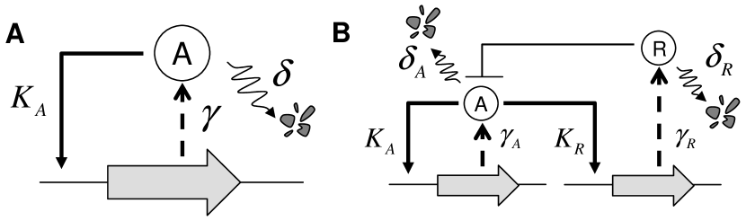
Figure 1: (A) A positive-feedback loop capable of maintaining two stable states Isaacs et al. (2003). (B) An excitable oscillator that exhibits noise-induced oscillations Vilar et al. (2002); Atkinson et al. (2003). The autoactivator triggers the production of a repressor $R$ that provides negative feedback control. (The dashed arrows denote lumped transcription and translation, the bold solid arrows denote activation, the blunt arrow denotes repression and the wavy arrows denote degradation.)

I.1 Autoactivator

Perhaps the simplest circuit motif able to exhibit multiple stable states is the autoactivating positive feedback loop (Figure 1a) J. E. Ferrell (2002). The circuit consists of a single gene encoding an activator. Several autoactivator circuits have been experimentally characterized, including the autoactivation of CI protein by the $P_{RM}$ promoter of phage $\lambda$ studied by Isaacs et al. Isaacs et al. (2003), and the autoactivation of NtrC by the glnAp promoter of E. coli studied by Atkinson et al. Atkinson et al. (2003). The autoactivator circuit is expected to exhibit either a HIGH state characterized by an elevated level of protein synthesis, or a LOW state characterized by a low basal level of production. We simplify the model by assuming that the activator binding and mRNA turnover are fast compared to the lifetime of the protein activator. The effect of the activator is quantified by the activation function $g\left({A/K_{A},f}\right)$ where $A$ is the activator concentration, $K_{A}$ is the equilibrium dissociation constant of the activator and its cognate binding site, and $f$ is the maximum fold-activation in the circuit. As a particular example, we assume a Hill-form for the activation function $g\left({A/K_{A},f}\right)$,

$$g\left({\frac{A}{{K_{A}}},f}\right)=\frac{{f^{-1}+\left({\frac{A}{{K_{A}}}}\right)^{n}}}{{1+\left({\frac{A}{{K_{A}}}}\right)^{n}}},$$ (1)

with cooperative activation ($n=2$) Bintu et al. (2005). The resulting model is a single kinetic equation governing the activator concentration $A(t)$ Keller (1995); Isaacs et al. (2003)(Figure 1a),

$$\frac{dA}{dt}=\gamma\cdot g(A)-\delta\cdot A,$$ (2)

where $\gamma$ is the fully activated rate of protein synthesis and $\delta$ is the protein degradation rate (which in prokaryotes is often estimated from the growth rate due to growth-mediated dilution).

In the deterministic limit, when the number of reactant molecules is very large, we expect Eq. 2 to adequately describe the system behavior. Once initial transients have died out, the system will approach a steady-state, and $A$ reaches its steady-state value $A_{s}$ where the rate of synthesis and degradation balance, i.e. $\gamma\cdot g(A_{s})=\delta\cdot A_{s}$. The stability of the steady-state is determined by the response of the system to a small perturbation $A_{p}$, found by linearizing Eq. 2 about $A_{s}$,

$$\frac{{dA_{p}}}{{dt}}=\left[{\gamma\cdot g^{\prime}\left({A_{s}}\right)-\delta}\right]\cdot A_{p}\equiv\lambda\cdot A_{p}.$$ (3)

The expression in the square brackets $\lambda\equiv\left[{\gamma\cdot g^{\prime}\left({A_{s}}\right)-\delta}\right]$ is a constant that depends upon the model parameters. If $\lambda$ is positive, the small perturbations will grow in time ($A_{s}$ is an unstable state), while if $\lambda$ is negative, the small perturbation will decay ($A_{s}$ is a stable state). In the stable case, the long-term state of the system can be thought of as a point located at the bottom of a valley (or basin of attraction) – the more negative the constant $\lambda$, the steeper the valley. As the model parameters are varied, the valley may become more flat ($\lambda\approx 0$) or even develop into a mountain ($\lambda>0$), resulting in a loss of stability. The parameter space is divided into regions of different qualitative behavior (as in Figure 2a, black curve); the threshold between these domains indicates where $\lambda$ has changed sign and is called the phase boundary. Although the model seems to depend upon a large family of parameters ($\gamma,\delta,K_{A}$, etc.), the stability of the deterministic model is actually described by two dimensionless combinations of these parameters: the ratio of the protein concentration with fully activated promoter ($A_{0}=\gamma/\delta$) to the dissociation constant, $A_{0}/K_{A}$, and the fold-activation, $f$.

The effective stability approximation (ESA) we propose is an approximation that allows the average effect of intrinsic noise to be expressed as a positive correction to $\lambda$,

$$\lambda^{\prime}=\lambda+\lambda_{corr}\quad\left({\lambda_{corr}>0}\right),$$ (4)

(see Eq. 15 below). The correction reflects an effective flattening of the local landscape by stochastic fluctuations, making it easier for the system to escape from the basin of attraction. Adopting this perspective allows the analysis used to study the deterministic model to be extended to the stochastic model with only minor modification. With $\lambda^{\prime}$ corrected to include the effect of the intrinsic noise, the new phase boundaries are drawn to coincide with points in parameter space where $\lambda^{\prime}=0$.

A major source of intrinsic noise in gene regulatory networks is so-called translational bursting Thattai and van Oudenaarden (2001); Kaern et al. (2005), where each mRNA transcript is translated into several peptides before the message is degraded, leading to a burst of protein synthesis. Typical values of the ‘burst size’ $b$ can vary from close to zero for poorly translated genes Ozbudak et al. (2002), up to several dozen Kennell and Riezman (1977); Cai et al. (2006) depending upon the rate of translation and the lifetime of the transcript. When intrinsic noise is included in the autoactivator model, and the procedure described in detail in Section III–A of the Supplementary Material is applied, we find the correction to $\lambda$ is $\lambda_{corr}\propto\Delta_{b}/\lambda^{2}$ where,

$$\Delta_{b}=\frac{(b+1)}{2}\frac{1}{K_{A}\;V_{cell}}=\frac{(b+1)}{2}\frac{1}{N_{A}},$$ (5)

is a third dimensionless quantity we call the discreteness parameter. This parameter captures the average change in protein number when a synthesis or degradation event occurs, scaled relative to the protein number required to initiate activation $N_{A}=K_{A}\times V_{cell}$, where $K_{A}$ is the activator dissociation constant and $V_{cell}$ is the cell volume. Increasing the discreteness parameter $\Delta_{b}$ increases the magnitude of the discrete change in activator numbers, and therefore increases the relative magnitude of the perturbation to the system caused by the intrinsic noise. One would expect the circuit to switch more readily from stable state to stable state as the magnitude of the intrinsic noise is increased, thereby reducing the average stability of the circuit. On the other hand, as the number of activator molecules increases $(N_{A}\to\infty)$, the discreteness parameter vanishes and the behavior of the system is fully described by the deterministic model. Thus, the discreteness parameter $\Delta_{b}$ represents a distillation of the complicated effect of intrinsic noise on the model behavior, captured in a compact expression that would be difficult to extract from numerical simulation data.

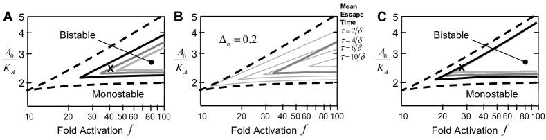
Figure 2: Stability phase plot for the autoactivator (Figure 1a), including the effect of intrinsic noise. (A) The black dashed curve is the phase boundary of the deterministic model with transcriptional activation ($A_{0}/K_{A}$ is the fully activated protein concentration scaled by the activator/DNA dissociation constant). Increasing the level of intrinsic noise by increasing the discreteness parameter $\Delta_{b}$ (i.e. increasing the ‘burstiness’ of translation or decreasing the number of molecules) diminishes the parameter regime of reliable bistability ($Re[\lambda^{\prime}]<0$). Here, $\Delta_{b}=0.1$ (black solid), 0.2 (dark gray) and 0.3 (light gray). (B) The average escape time from the stable state is an indicator of the permanence of the bistability. Here, the dark gray curve from Figure 2a corresponds to an escape time of about $\tau=6$, where time has been scaled relative to the protein lifetime $\delta^{-1}$. (C) As in Figure 2a, but now with translational activation. The range of bistability is considerably widened as transitions from the LOW to the HIGH state are supressed. Here, $K_{A}\cdot V_{cell}=25$ molecules and the fully activated burst size is $b=4$ (black), $b=9$ (dark gray) and $b=14$ (light gray).

As shown in Figure 2a, for the autoactivator the parameter space is divided into regions of bistability (two stable states) and monostability (one stable state). The bistability is most easily lost near the phase boundary separating the bistable and monostable states. The circuit parameters of Isaacs and co-workers Isaacs et al. (2003) lie close to the left-hand tip of the black triangle in Figure 2a ($f\approx 10$), and as they observed in their experiments, the noise overwhelms bistability in such a system (c.f. Figure 2A of Isaacs et al. (2003)), leading to rapid transitions between the stable states. A much greater fold-activation is required to maintain two distinct stable states (as likewise noted by the authors).

Actually, once noise is allowed in the autoactivator model, one no longer has stability in the strictest sense because there is always a chance that a perturbation will switch the system from one steady-state to the other. With noise, it is not a question of stability, but rather the average escape time from the steady-state Aurell and Sneppen (2002); Walczak et al. (2005). The longer the escape time (compared with other time scales in the problem), the more ‘stable’ the system. To emphasize the effect of the intrinsic noise on the stability phase plot, we consider a system with a small number of activator proteins $(K_{A}\cdot V_{cell}=25$ molecules). Using the parameters $\gamma=2\;\mbox{protein}\;\mbox{min}^{-1}$, $\delta^{-1}=30\;\mbox{min}$ (a half-life of $\sim 20\;\mbox{min}$), $K_{A}=25\;nM$ and a burst size of $b=10$, the discreteness parameter in E. coli ($V_{cell}\approx 1\mu m^{3}$) is $\Delta_{b}\approx 0.2$. From Figure 2a (dark gray curve), a maximum fold-activation of $f\geq 40$ is necessary to ensure long-lived bistable states (shown as a cross on the plot). It is possible to explicitly compute the average escape time from the stable states for this simple model (see Gardiner (2004); Kepler and Elston (2001) and Section II of the Supplementary Material). Figure 2b compares the average escape time as a function of $A_{0}/K_{A}$ and $f$ for the case above, with $\Delta_{b}=0.2$ (dark gray curve in Figure 2a). Along the dark gray curve, the escape time is $\tau=(3\pm 0.5)\;h$, which is about six times longer than the protein lifetime (which sets the basic time scale of the system’s ‘memory’).

The escape time is an indirect measure of the system’s stability. We have developed a more direct method that measures the effective rate of divergence of an ensemble of stochastic trajectories. This method is of general applicability and allows a direct evaluation of the accuracy of the ESA. The details of that calculation are reserved for the Supplementary Material (see Section III-A.2). Comparing $\lambda^{\prime}$ to the effective rate of divergence in the stochastic simulations of the autoactivator, the ESA is found to be accurate for systems with $\Delta_{b}\lesssim 0.25$.

The burst size $b$ can be reduced by decreasing the rate of translation and indeed Ozbudak et al. suggest that many poorly translated genes in E. coli could be the result of evolutionary selection against burst noise Ozbudak et al. (2002). Alternatively, the method of control in the circuit can be shifted from transcriptional to translational activation. Although the simple deterministic model remains unchanged for either choice of trancriptional or translational control, the resulting stochastic model exhibits improved stability for translational activation.

Figure 2c shows the result of putting the translation rate under control of the activator. Decreasing the translation rate in the LOW state has the effect of shifting the upper branch of the phase boundary, indicating a decrease in transitions from the LOW to the HIGH state. The translational autoactivator can tolerate a larger range of transcription rates (i.e. higher $\gamma$) and a lower maximum fold-activation ($f\geq 20$), even for large burst size. As above, with $\gamma=2\;\mbox{protein}\;\mbox{min}^{-1}$, $\delta^{-1}=30\;\mbox{min}$, $K_{A}=25\;nM$, $V_{cell}=1\;\mu m^{3}$ and a fully activated burst size $b=10$, a fold-activation of $f\geq 25$ is required to sustain the bistability (shown as a cross on the plot), almost half that required in the transcriptional autoactivator above.

To generate the phase plot for a given stochastic model requires division of the parameter space of the model (Eq. 2) into a fine grid, with stochastic simulation performed at each point. Even after several such simulations are generated, it is unlikely that the discreteness parameter $\Delta_{b}$ will suggest itself as a key measure of the magnitude of intrinsic noise. The ESA method provides not only a rapid overview of the parameter space, but provides compact expressions characterizing the effect of intrinsic noise on the observable dynamics. In the next section, we shall apply ESA to the analysis of a more elaborate circuit model.

I.2 Genetic oscillator

Oscillating systems underlie many physiological processes in the cell, from circadian rhythms Goldbeter (1997) to the cell cycle itself Pomerening et al. (2005). In addition to the natural systems, several synthetic genetic oscillator designs have been studied, including the mutually-repressing ring-oscillator (Repressilator) of Elowitz and Leibler Elowitz and Leibler (2000) and the activator-repressor design of Atkinson and co-workers Atkinson et al. (2003) (which has a great deal in common with the model discussed below). A recurring motif in experimentally characterized networks is a negative feedback loop serving as a system reset Goldbeter (1997); Dunlap (1999). Without some time delay or intervening mechanism to prevent reversibility, the system will rapidly approach an intermediate equilibrium, and it is found both theoretically Pomerening et al. (2003) and experimentally Pomerening et al. (2005) that a negative feedback loop alone is not sufficient to maintain reliable oscillations. If, however, the feedback repressor is controlled by a bistable autoactivator, the oscillations become more robust and coherent since the bistable switch acts as a ratchet that ‘locks’ into the HIGH state generating a large amount of repressor to feed back and reset the system to the LOW state where the system remains until the activator accumulates over a critical threshold to initiate another cycle Cross and Siggia (2005). This motif is highly represented in natural gene networks Dunlap (1999), and we shall use the ESA to ascertain the contribution of intrinsic noise to the performance of such an oscillator.

We consider the generic model proposed by Vilar and co-workers to describe circadian rhythms in eukaryotes Vilar et al. (2002), with a transcriptional autoactivator driving expression of a repressor that provides negative control by sequestering activator proteins through dimerization Steuer et al. (2003); Guantes and Poyatos (2006). The repressor and activator form an inert complex until the activator degrades, recycling repressor back into the system. In their model, the degradation rate of the activator, $\delta_{A}$, is the same irrespective of whether it is bound in the inert complex or free in solution. We simplify their original model somewhat, and as in the previous section, we assume fast activator/DNA binding and rapid mRNA turnover, leading to a reduced set of rate equations governing the concentration of activator $A$, repressor $R$ and the inert dimer $C$,

$$\frac{{dA}}{{dt}} = \gamma_{A}\cdot g\left({\frac{A}{{K_{A}}},f_{A}}\right)-\delta_{A}\cdot A-\kappa_{C}\cdot A\cdot R$$

$$\frac{{dR}}{{dt}} = \gamma_{R}\cdot g\left({\frac{A}{{K_{R}}},f_{R}}\right)-\delta_{R}\cdot R-\kappa_{C}\cdot A\cdot R+\delta_{A}\cdot C$$

$$\frac{{dC}}{{dt}} = \kappa_{C}\cdot A\cdot R-\delta_{A}\cdot C.$$ (6)

We further assume no cooperativity in activator binding ($n=1$ in the activation function $g$) and the nominal parameter set used in Vilar et al. (2002). For this more complicated system, there is a larger number of dimensionless combinations of parameters that characterize the system dynamics. The scaled repressor degradation rate $\epsilon=\delta_{R}/\delta_{A}$ is a key control parameter in the model since oscillations occur in the deterministic system only for an intermediate range of this parameter. For the nominal parameter set used in  Vilar et al. (2002), the deterministic model exhibits oscillations over the range $0.12<\epsilon<40$ (Figure 3a, black region). We shall focus on the parameter regime near to the phase boundary at $\epsilon\approx 0.12$ and examine the role intrinsic noise plays in generating regular oscillations from a deterministically stable system.

Applying the ESA to the oscillator model, the parameter $\Delta_{b_{A}}=(b_{A}+1)/(2\cdot K_{A}\cdot V_{cell})$ emerges as an important measure quantifying the discreteness in activator synthesis (see Eq. 36 in the Supplementary Material). Here again, $b_{A}$ is the burst size in the activator synthesis, $K_{A}$ is the activator/DNA dissociation constant and $V_{cell}$ is the cell volume. (Here, $V_{cell}=100\mu m^{3}$ as is appropriate for eukaryotic cells.)

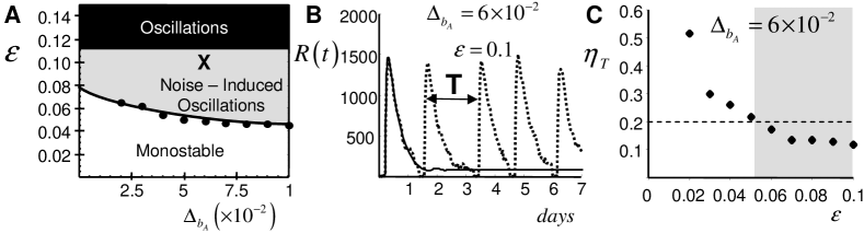
Figure 3: (A) Stability phase plot as a function of the scaled repressor degradation rate $\epsilon=\delta_{R}/\delta_{A}$ for the circuit shown in Figure 1b. The discreteness in the activator synthesis, $\Delta_{b_{A}}$, characterizes the average discrete change in activator concentration during each reaction, and consequently the magnitude of the intrinsic noise. The intrinsic noise expands the region of instability (gray) extending the parameter range over which oscillations are expected to occur. The deterministic phase boundary is located at $\epsilon\approx 0.12$ (dashed line separating the black and gray regions). The solid line is the phase boundary predicted from the roots of Eq. 14 and filled circles denote the phase boundary found by stochastic simulation (see text). The model and parameters are as in Vilar et al. Vilar et al. (2002). (B) The circuit exhibits noise-induced oscillations (dotted line) with inter-spike time $T$. The parameters used in the simulation correspond to a deterministically stable system (black line). Numerical simulation data was generated using Gillespie’s direct method Gillespie (1977), with parameters as used in Vilar et al. (2002) and $\epsilon=0.1,\Delta_{b_{A}}=6\times 10^{-2}$ (cross in Figure 3b). (See Section III–C of the Supplementary Material.) (C) A plot of the noise-to-signal ratio $\eta_{T}=\langle{\left({\langle T\rangle-T}\right)^{2}}\rangle^{1/2}/\langle T\rangle$ as a function of $\epsilon$. The oscillations are regular when $\eta_{T}$ is small (the region of noise-induced oscillations predicted by the ESA is gray), and $\eta_{T}$ was calculated using at least 200 spikes for each point.

Using the nominal parameter set of Vilar et al. Vilar et al. (2002) in our reduced model leads to a burtiness in activator synthesis of $b_{A}=5$ (giving $\Delta_{b_{A}}=6\times 10^{-2}$) and a burstiness in repressor synthesis of $b_{R}=10$. The phase boundary predicted by the ESA is shown as a solid line in Figure 3a, bounding a region of parameter space between the deterministic phase boundary where qualitatively different behavior is expected from the stochastic model. We examine the system behavior in this region by running a stochastic simulation using the parameter choice $\epsilon=0.1$ and $\Delta_{b_{A}}=6\times 10^{-2}$ (denoted by a cross in Figure 3a). With this choice, the deterministic model is stable (Figure 3b, black line). Nevertheless, a stochastic simulation of the same model, including protein bursting and stochastic dimerization, clearly shows oscillations (Figure 3b, dotted line).

The time between successive peaks in the stochastic simulation of Figure 3b is denoted by $T$. As is clear from Figure 3b, $T$ is itself a random variable. Each simulation run generates a collection of inter-spike times from which the mean $\langle T\rangle$ and the variance $\langle{\left({\langle T\rangle-T}\right)^{2}}\rangle^{1/2}$ can be calculated. Following Steuer et al. Steuer et al. (2003), the quality of the noise-induced oscillations is measured using the noise-to-signal ratio $\eta_{T}=\langle{\left({\langle T\rangle-T}\right)^{2}}\rangle^{1/2}/\langle T\rangle$, and the system is said to exhibit regular oscillations where $\eta_{T}$ is small Steuer et al. (2003); Guantes and Poyatos (2006). The dependence of $\eta_{T}$ on the repressor degradation rate $\epsilon$ is shown in Figure 3c, with the discreteness parameter $\Delta_{b_{A}}=6\times 10^{-2}$ (as in Figure 3b), using at least 200 spikes to calculate $\eta_{T}$. At low repressor degradation rate, the noise-to-signal ratio is high, indicating large variance in the inter-spike time $T$ and corresponding to a stable (i.e., non-oscillatory) system. As the repressor degradation rate is increased, the variance in the inter-spike time $T$ decreases with a consequent decrease in the noise-to-signal ratio $\eta_{T}$, indicative of a more regularly oscillating system. Physically, the intrinsic noise in this parameter range is sufficient to drive the system away from the deterministically stable steady-state, yet the noise is not so strong that the return trajectory through phase space is much affected.

As in the autoactivator model, it is useful to compare the phase boundary predicted by the ESA to some independent measure of stability, in this case $\eta_{T}$. In Figure 3c, the ESA phase boundary (for $\Delta_{b_{A}}=6\times 10^{-2}$) is denoted by the interface between the white and gray regions, corresponding to a value of $\eta_{T}\approx 0.2$. Using data such as that shown in Figure 3c, the points in the phase plot with $\eta_{T}=0.2$ can be found for a range of discreteness parameter $\Delta_{b_{A}}$ (Figure 3a, filled circles). These points correspond very well to the phase boundary calculated using the ESA (Figure 3a, solid line). The results are as one would expect – near the deterministic phase boundary, very little molecular noise is required to sustain oscillations, and reasonable periodicity persists even for small values of the discreteness parameter ($\Delta_{b_{A}}\to 0$, $b_{R}\neq 0$). As the repressor degradation rate $\epsilon$ is decreased to a region favoring stability, more noise is required to overcome the deterministic stability of the system and initiate the autoactivator trigger. It is illustrative to remark that each data point in Figure 3a, obtained from stochastic simulation Gillespie (1977), took roughly a day to generate on a dual processor desktop computer since at low repressor degradation rate, a large separation of timescales is introduced necessitating long stochastic simulation runs to capture the slowly-varying dynamics of the system. By contrast, the solid line generated from the roots of Eq. 14, took less than an hour to produce on the same machine. Thus, even for a two-gene circuit with several degrees of freedom, the ESA affords a compact and convenient means to survey the phase space, drawing attention to those regions of particular interest that may be probed in more detail by more realistic (though also more computationally costly) stochastic simulation methods.

II Methods

The effective stability approximation can be applied to generic models of genetic circuits in a straightforward way. Here, a brief outline of the method is provided. A self-contained tutorial on stochastic modeling and the ESA is found in the Supplementary Material.

A useful abstraction of genetic regulatory networks is as a system of ordinary differential equations Conrad and Tyson (2006); Kaern and Weiss (2006). (Here, and throughout, we shall assume a spatially homogeneous environment.) We denote the concentrations of the reactants of interest by the state vector ${\bf x}$, where the $x_{i}$ correspond to the concentration of mRNA, transcription factors, protein products, etc. The kinetic equation governing the evolution of the system takes the form $\frac{d{\bf x}}{dt}={\bf f}({\bf x})$, where ${\bf f}$ is a vector of nonlinear functions of the state variables. We can estimate the long-time, or steady-state, behavior of the model by first computing the equilibrium points ${\bf x}_{s}$ that satisfy the algebraic constraint ${\bf f}({\bf x}_{s})={\bf 0}$. We then Taylor expand the reaction rate vector about the equilibrium point by making the substitution ${\bf x}={\bf x}_{s}+{\bf x}_{p}$ (where ${\bf x}_{p}$ is an infinitesimal perturbation away from ${\bf x}_{s}$), and retain only linear terms in ${\bf x}_{p}$. The resulting dynamics of ${\bf x}_{p}$ are given by$\frac{d}{dt}{\bf x}_{p}={\bf J}\cdot{\bf x}_{p}$, where ${\bf J}$ is the Jacobian or response matrix: ${\bf J}_{ij}=\partial f_{i}/\partial x_{j}$. The eigenvalues of ${\bf J}$ are the matrix analogue of the parameter $\lambda$ introduced in Eq. 3, and in a similar fashion if the eigenvalues all have negative real-part, then ${\bf x}_{s}$ is a stable steady state. (There are, of course, limitations to how far one can trust the linearization Strogatz (1994), but for our purposes it is sufficient as a first approximation.)

To include stochastic effects in the mathematical model, chemical reaction rates must be re-written in terms of the reaction propensity and stoichiometry Gillespie (1977). For example in the positive autoactivator example above, with the individual synthesis and degradation stoichiometries written explicitly, the deterministic model equations (Eq. 2) read,

$$\begin{array}[]{*{20}c}{\mbox{bursty synthesis:}}&{A\xrightarrow{{\nu_{1}}}A+b;}&{\nu_{1}=\frac{{\gamma}}{b}\cdot g\left(A\right)},\\ {\mbox{linear degradation:}}&{A\xrightarrow{{\nu_{2}}}A-1;}&{\nu_{2}=\delta\cdot A.}\\ \end{array}$$ (9)

We encode this information concisely as the propensity vector $\bm{\nu}=[\nu_{1},\nu_{2}]=[{\gamma\cdot g(A)/b,\delta\cdot A}]$ and the stoichiometry matrix ${\bf S}=[b,-1]$. The discrete change in molecule numbers following the completion of a chemical reaction causes a deviation from the deterministic solution since the deterministic model assumes an infinitesimally small and continuous change in the state. (Consequently, the deterministic model only applies to systems with large numbers of molecules.) We denote the deviation of the stochastic model from the deterministic model by the fluctuating quantity $\omega\cdot\bm{\alpha}(t)$, where $\omega=1/\sqrt{V_{cell}}$ and $\bm{\alpha}(t)$ describes the stochastic deviation in each species ${\bf x}$. The $\sqrt{V_{cell}}$ scaling arises from the observation that the relative magnitude of the intrinsic noise scales roughly as the inverse square-root of the number of molecules van Kampen (1976a). Elf and Ehrenberg Elf and Ehrenberg (2003) have developed an algorithmic expression for the statistics of $\bm{\alpha}$ using the linear noise approximation of van Kampen van Kampen (1976a). In that formulation, the mean and covariance of the fluctuations about the deterministic state are written compactly in terms of the propensity vector $\bm{\nu}$ and the stoichiometry matrix ${\bf S}$; here, we shall apply their method to characterize the fluctuations about the stable state. The first step in the calculation of the moments of the fluctuations $\omega\bm{\alpha}(t)$ is to construct the auxiliary matrices ${\bf\Gamma}$ and ${\bf D}$, evaluated at the stable state ${\bf x}_{s}$,

$$\Gamma_{ij}(t)=\frac{\partial[{{\bf S}\cdot{\bm{\nu}}}]_{i}}{\partial x_{j}}=\frac{{\partial f_{i}}}{{\partial x_{j}}}\quad\quad{\bf D}={\bf S}\cdot\mbox{diag}[{\bm{\nu}}]\cdot{\bf S}^{T}.$$ (10)

The drift matrix ${\bf\Gamma}={\bf J}$ is the response matrix (or Jacobian) described above and reflects the local stability of the deterministic system to small perturbations Ali and Menzinger (1999). The diffusion matrix ${\bf D}$ captures the strength of the fluctuations and is related to the magnitude of the reaction step-size Elf and Ehrenberg (2003); Scott et al. (2006). It is straightforward to show that to leading-order in $\omega$ the mean of the fluctuations is zero ($\langle\bm{\alpha}\rangle=\bm{0}$) and the variance, denoted by the symmetric matrix ${\bm{\Xi}}=\langle{\bm{\alpha}}\cdot{\bm{\alpha}}^{T}\rangle$, is determined by the solution of the system of algebraic equations van Kampen (1976a), ${\bf{\Gamma}}\cdot{\bf{\Xi}}+{\bf{\Xi}}\cdot{\bf{\Gamma}}^{T}+{\bf{D}}={\bf 0}$. Since the fluctuations about the stable state are stationary, the time autocorrelation function depends upon the time difference only, and is given by the matrix exponential,

$$\left\langle{{\bm{\alpha}}\left(t\right){\bm{\alpha}}^{T}\left({t-\tau}\right)}\right\rangle=\exp\left[{{\bf{\Gamma}}\tau}\right]\cdot{\bf{\Xi}}.$$ (11)

The effect of the fluctuations on the deterministic steady-state is calculated by including an additional term in the deterministic linearization above: ${\bf x}={\bf x}_{s}+{\bf x}_{p}+\omega{\bm{\alpha}}$. Linearizing ${\bf J}$ in $\omega$, we have a stochastic differential equation governing the decay of the perturbation modes ${\bf x}_{p}$,

$$\frac{d}{dt}{\bf x}_{p}=[{{\bf J}^{(0)}+\omega\;{\bf J}^{(1)}(t)}]\cdot{\bf x}_{p}.$$ (12)

The fluctuations affect the decay of the infinitesimal disturbance ${\bf x}_{p}$ as well as the dynamics of the average $\langle{\bf x}_{p}\rangle$, which (provided $\omega\;{\bf J}^{(1)}(t)\ll{\bf J}^{(0)}$) is approximately governed by the convolution equation Bourret (1965); van Kampen (1976b),

$$\frac{d}{{dt}}\left\langle{{\bf x}_{p}\left(t\right)}\right\rangle={\bf J}^{(0)}\left\langle{{\bf x}_{p}\left(t\right)}\right\rangle+\omega^{2}\int\limits_{0}^{t}{{\mathbf{J}}_{c}\left(t-\tau\right)\left\langle{{\bf x}_{p}\left({\tau}\right)}\right\rangle d\tau},$$ (13)

where ${\mathbf{J}}_{c}\left(t-\tau\right)=\left\langle{{\mathbf{J}}^{\left(1\right)}\left(t\right)e^{{\mathbf{J}}^{\left(0\right)}(t-\tau)}{\mathbf{J}}^{\left(1\right)}\left(\tau\right)}\right\rangle$ is made up of linear combinations of the cross-correlations $\langle\alpha_{i}(t)\alpha_{j}(\tau)\rangle$ given by the $i^{th}$ row and the $j^{th}$ column of the right-hand side of Eq. 11. In the noiseless case, the stability of the perturbation ${\bf x}_{p}$ is determined by the eigenvalues of ${\bf J}^{(0)}$: $\mbox{diag}\{\lambda_{i}\}={\bf P}^{-1}\cdot{\bf J}^{(0)}\cdot{\bf P}$ where the matrix ${\bf P}$ is made of the eigenvectors of ${\bf J}^{(0)}$. The analogues of the eigenvalues for the convolution equation above are found from the poles of the Laplace transform, denoted $\lambda^{\prime}$, which solve the resolvent equation Grossman and Miller (1973),

$$\det\left[{\lambda^{\prime}{\mathbf{I}}-{\mathbf{J}}^{\left(0\right)}-\frac{1}{V_{cell}}{\mathbf{\hat{J}}}_{c}\left({\lambda^{\prime}}\right)}\right]=0,$$ (14)

Here $\omega^{2}$ has been replaced by $V^{-1}_{cell}$ and ${\mathbf{\hat{J}}}_{c}\left(s\right)=\int\limits_{0}^{\infty}{{\bf J}_{c}(t)e^{-st}dt}$ is the Laplace transform of ${\bf J}_{c}(t)$. If the deterministic eigenvalues are distinct, we can further approximate the effective eigenvalue $\lambda^{\prime}_{i}$ by,

$$\lambda^{\prime}_{i}=\lambda_{i}+\frac{1}{V_{cell}}\;[\;{\bf P}^{-1}\cdot{\mathbf{\hat{J}}}_{c}\left(\lambda_{i}\right)\cdot{\bf P}\;]_{ii}.$$ (15)

where $[\;\cdot\;]_{ii}$ denotes the $i^{th}$ diagonal entry of the matrix. Physically, we interpret the leading-order noise correction as the power in the fluctuations at eigenfrequency $\lambda_{i}$ projected in the eigendirection of $\lambda_{i}$. Since the correction term is quadratic, it is always positive and thus de-stabilizes the eigenmode upon which it is projected. (Hence, in Eq. 4 we write $\lambda_{corr}>0$.)

It often happens that out of the term $1/V_{cell}\;[\;{\bf P}^{-1}\cdot{\mathbf{\hat{J}}}_{c}\left(\lambda_{i}\right)\cdot{\bf P}\;]_{ii}$ there appears a small parameter that quantifies the effect of the intrinsic noise. (For the two examples above, the small parameters are $\Delta_{b}$ and $\Delta_{b_{A}}$, each characterizing the discreteness of the protein change.) In the limit that this parameter goes to zero, the effect of the intrinsic noise becomes negligible, at least in that particular eigenmode.

Finally, the ESA can be easily implemented in a symbolic computational environment, without attending to the mathematical details (see Section IV of the Supplementary Material). A version of the ESA coded in Mathematica is freely available from the authors by request.

III Supplementary Material

Much theoretical work has been devoted to quantifying the conditions under which microscopic fluctuations have macroscopic effects Horsthemke and Lefever (1984). The most useful results are often restricted to systems with a single degree of freedom or employ sophisticated tools such as Itô’s calculus. In what follows, we aim to develop a convenient and simple scheme to assess the stability properties of a dynamical system subject to molecular noise described by the chemical Master equation. The method is an extension of the familiar linear stability analysis of nonlinear dynamical systems, although here the effective eigenvalues about the equilibrium points are adjusted to reflect the influence of the noise.

IV Mathematical Methods

A very useful qualitative picture of the behavior of a system of nonlinear differential equations emerges from the linearized dynamics about the fixed-point(s) (also called the steady-state(s)) of the system, defined as the reactant concentrations at which the synthesis and degradation rates balance. The stability of the system near the fixed-points can be estimated by calculating the eigenvalues $\{\lambda_{i}\}$ of the resulting linearization, which are generally a set of complex numbers. If the real parts are all negative, we say the system is locally stable, meaning small perturbations away from the steady-state are automatically corrected.

Since genetic circuits, both natural and engineered, rely upon transfer of information through small numbers of molecules, significant fluctuation is simply one of the inherent operating conditions Kerszberg (2004), resulting in noise that may give rise to behavior that is very different from the behavior predicted by deterministic models. Consequently, for cell-scale modeling we propose to modify the deterministic notion of stability by calculating the effective eigenvalues $\lambda^{\prime}_{i}$, which include the averaged influence of the intrinsic noise,

$$\lambda_{i}^{\prime}=\lambda_{i}+\lambda_{corr}.$$ (16)

Here $\lambda_{corr}\propto V_{cell}^{-1}$ is inversely proportional to the cell volume $V_{cell}$ For notational convenience in the following, we introduce a parameter $\omega$ that is related to the cell volume by: $\omega^{-2}=V_{cell}$. Sometimes $\omega^{-2}$ is called the ‘system size’, expressing as it does the relationship between reactant concentration and molecule numbers Elf and Ehrenberg (2003); van Kampen (1992).

IV.1 Stochastic stability equation

To calculate the stability of the macroscopic model $\frac{d{\bf x}}{dt}={\bf f}({\bf x})$ to small perturbations, the system is linearized about the equilibrium point: ${\bf x}={\bf x}_{s}+{\bf x}_{p}$,

$$\frac{d}{{dt}}{\bf{x}}_{p}={\bf{J}^{(0)}}\cdot{\bf{x}}_{p}.$$ (17)

(Here, and henceforth, we adopt the convention of writing all matrix variables in bold upper-case, and all vectors in bold lower-case.) The eigenvalues of the Jacobian ${\bf{J}}^{(0)}=\left.{\frac{{\partial{\bf{f}}}}{{\partial{\bf{x}}}}}\right|_{{\bf{x}}={\bf{x}}_{s}}$ provide the decay rate of the exponential eigenmodes; if all the eigenvalues have negative real part, we say the system is locally asymptotically stable. We shall restrict ourselves to this notion of stability, although it does ignore algebraically growing modes which may be important in certain instances Trefethen and Embree (2005).

To accommodate fluctuations on top of the small perturbation ${\bf x}_{p}$, we set ${\bf x}={\bf x}_{s}+{\bf x}_{p}+\omega{\bm{\alpha}}(t)$. The Jacobian

$${\bf J}\equiv\left.{\frac{{\partial{\bf{f}}}}{{\partial{\bf{x}}}}}\right|_{{\bf{x}}={\bf{x}}_{s}+\omega{\bm{\alpha}}},$$

will then be a (generally) nonlinear function of the fluctuations about the steady-state ${\bm{\alpha}}(t)$. (As a technical aside, we note that we are justified in replacing ${\bf x}$ by ${\bf x}_{s}+{\bf x}_{p}+\omega\bm{\alpha}(t)$ in both the right- and left-hand side of the deterministic model $\frac{d{\bf x}}{dt}={\bf f}({\bf x})$ since the fluctuations $\bm{\alpha}(t)$ have non-zero correlation time (as we show below) and zero mean, allowing us first to conclude that the time-derivative of $\bm{\alpha}(t)$ exists and further that the average of this derivative must vanish: $\langle{\frac{d\bm{\alpha}}{dt}}\rangle=\frac{d\langle\bm{\alpha}\rangle}{dt}=0$). In the limit $\omega\to 0$, we can further linearize ${\bf J}$ with respect to $\omega$,

$${\mathbf{J}}\approx\left.{\mathbf{J}}\right|_{\omega\to 0}+\omega\left.{\frac{{\partial{\mathbf{J}}}}{{\partial\omega}}}\right|_{\omega\to 0}\equiv{\mathbf{J}}^{(0)}+\omega{\mathbf{J}}^{(1)}\left(t\right).$$

The stability equation is then given by,

$$\frac{d}{{dt}}{\bf{x}}_{p}=[{\bf{J}^{(0)}}+\omega{\bf J}^{(1)}(t)]\cdot{\bf{x}}_{p}.$$ (18)

This is a linear stochastic differential equation with random coefficient matrix ${\bf J}^{(1)}(t)$ composed of a linear combination of the steady-state fluctuations ${\bm{\alpha}}(t)$ which have non-zero correlation time (cf. Eq. 11). We therefore need not appeal to any specialized calculi (e.g. Itô’s calculus) for interpretation since the non-vanishing correlation time of the fluctuations ensures that ${\bf{x}}_{p}$ is a differentiable process and the equation falls under the purview of ordinary calculus van Kampen (1981).

Our present interest is in the mean stability of the equilibrium point. Taking the ensemble average of Eq. 18,

$$\frac{d}{{dt}}\left\langle{{\bf{x}}_{p}}\right\rangle={\bf{J}}^{(0)}\cdot\left\langle{{\bf{x}}_{p}}\right\rangle+\omega\left\langle{{\bf{J}}^{(1)}\left(t\right)\cdot{\bf{x}}_{p}}\right\rangle.$$

The right-most term is the cross-correlation between the process ${\bf x}_{p}$ and the coefficient matrix ${\bf J}^{(1)}(t)$. Since the correlation time of ${\bf J}^{(1)}(t)$ is not small compared with the other time scales in the problem, it cannot be replaced by white noise, and an approximation scheme must be developed to find a closed evolution equation for $\langle{\bf x}_{p}\rangle$.

IV.2 Bourret’s mode-coupling approximation

By assumption, the number of molecules is large so the parameter $\omega$ is small, although not so small that intrinsic fluctuations can be ignored. To leading-order in $\omega$, the trajectory ${\bf x}_{p}\left(t\right)$ is a random function of time since it is described by a differential equation with random coefficients. Derivation of the entire probability distribution of ${\bf x}_{p}\left(t\right)$ is usually impossible, and we must resort to methods of approximation. We shall adopt the closure scheme of Bourret Bourret (1962, 1965); van Kampen (1976b) to arrive at a deterministic equation for the evolution of the averaged process $\left\langle{{\bf x}_{p}\left({t}\right)}\right\rangle$ in terms of only the first and second moments of the fluctuations. In that approximation, provided ${\bf J}^{(0)}\gg\omega{\bf J}^{(1)}$, the dynamics of $\langle{\bf x}_{p}\rangle$ are governed by the convolution equation,

$$\frac{d}{{dt}}\left\langle{{\bf x}_{p}\left(t\right)}\right\rangle={\bf J}_{0}\left\langle{{\bf x}_{p}\left(t\right)}\right\rangle$$ (19)

$$+\omega^{2}\int\limits_{0}^{t}{{\mathbf{J}}_{c}\left(t-\tau\right)\left\langle{{\bf x}_{p}\left({\tau}\right)}\right\rangle d\tau},$$

where ${\mathbf{J}}_{c}\left(t-\tau\right)=\left\langle{{\mathbf{J}}^{\left(1\right)}\left(t\right)e^{{\mathbf{J}}^{\left(0\right)}(t-\tau)}{\mathbf{J}}^{\left(1\right)}\left(\tau\right)}\right\rangle$ is the time autocorrelation matrix of the fluctuations and $e^{{\bf J}_{0}\tau}$ is the matrix exponential. The equation can be solved formally by Laplace transform,

$$\left\langle{{\bf{\hat{x}}_{p}}\left(s\right)}\right\rangle=\left[{s{\mathbf{I}}-{\mathbf{J}}^{(0)}-\omega^{2}{\mathbf{\hat{J}}}_{c}\left(s\right)}\right]^{-1}\left\langle{{\bf x}_{p}\left(0\right)}\right\rangle,$$

where now ${\mathbf{\hat{J}}}_{c}\left(s\right)=\int\limits_{0}^{t}{{\mathbf{J}}_{c}\left(t\right)e^{-st}dt}$. A necessary and sufficient condition for asymptotic stability of the averaged perturbation modes $\left\langle{{\bf x}_{p}\left(t\right)}\right\rangle$ is that the roots $\lambda^{\prime}$ of the resolvent,

$$\det\left[{\lambda^{\prime}{\mathbf{I}}-{\mathbf{J}}_{0}-\omega^{2}{\mathbf{\hat{J}}}_{c}\left(\lambda^{\prime}\right)}\right]=0,$$ (20)

all have negative real parts $(Re(\lambda^{\prime})<0)$ Miller (1971); Grossman and Miller (1973). Some insight into the behavior of the system can be gained by considering a perturbation expansion of the effective eigenvalues $\lambda^{\prime}$ in terms of the small parameter $\omega$. We further diagonalize ${\bf J}^{(0)}$, $\mbox{diag}[\lambda_{i}]={\bf P}^{-1}\cdot{\bf J}^{(0)}\cdot{\bf P}$, and provided the eigenvalues are distinct, we can explicitly write $\lambda^{\prime}_{i}$ in terms of the unperturbed eigenvalues $\lambda_{i}$ to $O(\omega^{4})$ as,

$$\lambda^{\prime}_{i}=\lambda_{i}+\omega^{2}\;[\;{\bf P}^{-1}\cdot{\mathbf{\hat{J}}}_{c}\left(\lambda_{i}\right)\cdot{\bf P}\;]_{ii},$$ (21)

where $[\;\cdot\;]_{ii}$ denotes the $i^{th}$ diagonal entry of the matrix.

Notice the matrix product ${\bf J}_{c}(t-\tau)$ contains linear combinations of the correlation of the fluctuations $\langle\alpha_{i}(t)\alpha_{j}(\tau)\rangle$, and as such we must derive an expression for those moments.

IV.3 Calculating the statistics of the steady-state fluctuations

The statistics of the fluctuations $\bm{\alpha}$ are fully determined by the solution of the chemical Master equation (defined below) that comes from treating each reaction event probabilistically. In that probabilistic formulation, our state at any time $t$ is represented by the vector of molecule numbers ${\mathbf{n}}\in\mathbb{N}^{d}$; with $n_{i}$ representing the number of molecules of a given species. Each reaction causes a transition from the initial state ${\bf n}$ to some new state ${\bf n}^{\prime}$ reflecting the addition or removal of molecules by that reaction. The probability that the transition ${\bf n}\to{\bf n}^{\prime}$ occurs is the product of the probability of being in state ${\bf n}$ at time $t$, $P({\bf n},t)$, and the transition probability of moving from ${\bf n}\to{\bf n}^{\prime}$, denoted by $W_{{\bf n}\to{\bf n}^{\prime}}$. We thus write the probability conservation as a balance of flux into and out of the state ${\bf n}$, which yields a discrete differential equation for $P({\bf n},t)$,

$$\frac{{\partial P\left({{\bf{n}},t}\right)}}{{\partial t}}=\sum\limits_{{\bf{n^{\prime}}}}{W_{{\bf{n^{\prime}}}\to{\bf{n}}}P\left({{\bf{n^{\prime}}},t}\right)-W_{{\bf{n}}\to{\bf{n^{\prime}}}}P\left({{\bf{n}},t}\right)}.$$ (22)

The evolution equation for $P({\bf n},t)$ is called the Master equation McQuarrie (1967). It is rare that the Master equation can be solved exactly for $P({\bf n},t)$, and approximation schemes are required. One such scheme, the linear noise approximation van Kampen (1976a), is versatile and will be described briefly (see also Elf and Ehrenberg (2003) and Scott et al. (2006)). The approximation begins with the assumption that the molecule concentrations can be meaningfully separated into a component that evolves deterministically, which we shall denote ${\bf x}(t)$, and fluctuations ${\bm{\alpha}}(t)$ that account for the deviation of the stochastic model from the deterministic model. We introduce a scaling parameter $\omega$, where $\omega^{-2}=V_{cell}$ is the volume of the cell and is an extensive measure of the number of molecules. We then make the ansatz that the fluctuations scale as the square-root of the number of molecules: $\omega^{2}\;n_{i}=x_{i}+\omega\;\alpha_{i}$ van Kampen (1976a); Kubo et al. (1973). In that way, a perturbation expansion as the number of molecules gets large ($\omega\to 0$, with concentration held fixed), returns to zero’th order the macroscopic reaction rate equations,

$$\frac{d\bf{x}}{dt}=\bm{f}(\bf{x}).$$ (23)

The first-order equation, that comes at $O(\omega)$, characterizes the probability distribution for the fluctuations $\Pi({\bm{\alpha}},t)$ centered on the macroscopic trajectory ${\bf x}(t)$, and has the form of a linear Fokker-Planck equation,

$$\frac{{\partial\Pi}}{{\partial t}}=-\sum\limits_{i,j}{\Gamma_{ij}{\partial_{i}}(\alpha_{j}\Pi)}+\frac{1}{2}\sum\limits_{i,j}{D_{ij}\partial_{ij}\Pi}.$$ (24)

where $\partial_{i}$ denotes ${\partial\mathord{\left/{\vphantom{\partial{\partial\alpha_{i}}}}\right.\kern-1.2pt}{\partial\alpha_{i}}}$ and

$$\Gamma_{ij}(t)=\frac{{\partial f_{i}}}{{\partial x_{j}}}\quad\quad\bm{D}={\bf S}\cdot\mbox{diag}[{\bm{\nu}}]\cdot{\bf S}^{T},$$ (25)

(see main text). The matrices $\bm{\Gamma}$ and $\bm{D}$ are independent of $\bm{\alpha}$, which appears only linearly in the drift term. As a consequence, the distribution $\Pi(\bm{\alpha},t)$ will be Gaussian for all time. In particular, at equilibrium the fluctuations are distributed with density,

$$\Pi_{s}\left({\bm{\alpha}}\right)=\left[{\left({2\pi}\right)^{d}\det{\mathbf{\Xi}}}\right]^{\frac{1}{2}}\exp\left[{-\frac{1}{2}{\bm{\alpha}}^{T}\cdot{\mathbf{\Xi}}^{-1}\cdot{\bm{\alpha}}}\right],$$

and variance ${\bf\Xi}=\langle{\bm{\alpha}}\cdot{\bm{\alpha}}^{T}\rangle$ determined by,

$${\bf{\Gamma}}\cdot{\bf{\Xi}}+{\bf{\Xi}}\cdot{\bf{\Gamma}}^{T}+{\bf{D}}=0.$$ (26)

Furthermore, the steady-state time correlation function is,

$$\left\langle{{\bm{\alpha}}\left(t\right){\bm{\alpha}}^{T}\left({t-\tau}\right)}\right\rangle=\exp\left[{{\bf{\Gamma}}\tau}\right]\cdot{\bf{\Xi}}.$$ (27)

Around the steady-state, the process is stationary, which means the correlation function depends upon time difference only. Also note that the characteristic correlation time $\tau_{c}=||{\bf\Gamma}||^{-1}$ is related to the Jacobian ${\bf\Gamma}$ of the deterministic equations, and therefore cannot be divorced from the deterministic relaxation time. As a consequence, representing the fluctuations ${\bm{\alpha}}(t)$ as white noise $(\tau_{c}\to 0)$ is not justified.

The great advantage of the linear noise approximation is that the autocorrelation function of the steady-state fluctuations can be calculated directly from the macroscopic reaction rates in an algorithmic fashion Elf and Ehrenberg (2003). Furthermore, since ${\bf\Gamma}$ and ${\bf D}$ are derived from the known propensity and stoichiometry of the reactions, the statistics of $\bm{\alpha}$ are fully determined and are not tunable by some ad hoc prescription.

V Mean first passage time

Bistability is a property exhibited by deterministic systems. In a stochastic context, bistability is sometimes assigned to an equilibrium probability distribution with two maxima, irrespective of their separation. A more practical criterion for bistability is that the two states are long-lived and that the mean escape time from one state to the other is longer than the natural timescales in the problem. For the single-variable autoactivator model, we are able to compute the escape time by an explicit (though approximate) expression (see  Kepler and Elston (2001) or p. 139 of Gardiner (2004) for details). Under fairly unrestrictive assumptions Gillespie (2000), the Master equation may be approximated by the nonlinear Fokker-Planck equation,

$$\frac{{\partial P\left({a,t}\right)}}{{\partial t}}=-\frac{\partial}{{\partial a}}\Gamma\left(a\right)P\left({a,t}\right)+\frac{1}{2}\frac{{\partial^{2}}}{{\partial a^{2}}}D\left(a\right)P\left({a,t}\right),$$

where the functions $\Gamma$ and $D$ are the nonlinear analogues of the coefficient matrices ${\bf\Gamma}$ and ${\bf D}$ generated by the linear noise approximation shown in the previous section. For our autoactivator example, the coefficients are given by,

$$\Gamma(a)=\gamma\cdot g(a)-\delta\cdot a\quad\quad D(a)=\gamma\cdot b\cdot g(a)+\delta\cdot a.$$

The nonlinear Fokker-Planck equation has no general solution for systems of dimension greater than 1, and even the stationary solution is often impossible to calculate exactly for such systems Risken (1989). In the reduced autoactivator model, we are fortunate to have a system with one independent variable, so we can write the stationary solution of the Fokker-Planck equation explicitly as,

$$P^{s}(a)=\frac{\mathcal{N}}{D(a)}\;\mbox{exp}\left[{2\int\limits_{0}^{a}{\frac{{\Gamma\left({a^{\prime}}\right)}}{{D\left({a^{\prime}}\right)}}da^{\prime}}}\right],$$

where $\mathcal{N}$ is the constant of normalization (see p. 124 of Gardiner (2004)). Furthermore, we can explicitly write the first passage time $\tau$ from the HIGH state to the LOW state or vice-versa.

$$\tau_{HI\to LO}=2\int\limits_{a_{mid}}^{a_{HI}^{*}}{\frac{1}{{\psi\left(x\right)}}\int\limits_{x}^{\infty}{\frac{{\psi\left(y\right)}}{{D\left(y\right)}}dy}dx}$$

$$\tau_{LO\to HI}=2\int\limits_{a_{LO}^{\star}}^{a_{mid}}{\frac{1}{{\psi\left(x\right)}}\int\limits_{0}^{x}{\frac{{\psi\left(y\right)}}{{D\left(y\right)}}dy}dx},$$

where $a_{mid}$ is the unstable equilibrium point separating the HIGH and LOW states $a^{\star}_{HI}$ and $a^{\star}_{LO}$, respectively. The function $\psi(x)$ is given by,

$$\psi(x)=\mbox{exp}\left[{2\int\limits_{0}^{x}{\frac{{\Gamma\left({x^{\prime}}\right)}}{{D\left({x^{\prime}}\right)}}dx^{\prime}}}\right],$$

(see p. 139 of Gardiner (2004) for additional details).

In the main text, we discuss $\mbox{min}[\tau_{LO\to HI},\tau_{HI\to LO}]$ along the stability curves predicted by the effective eigenvalues. For $\Delta_{b}=0.1$, $\mbox{min}[\tau_{LO\to HI},\tau_{HI\to LO}]=$$8\pm 4$, where time has been scaled to protein lifetime ($\delta^{-1}$). For $\Delta_{b}=0.2$ and $\Delta_{b}=0.3$, $\mbox{min}[\tau_{LO\to HI},\tau_{HI\to LO}]=5.6\pm 1.4$ and $5.9\pm 0.3$, respectively.

VI Details of Genetic Circuit Examples

VI.1 The autoactivator

We describe the transcription of the activator mRNA, $m_{a}$ and the translation of activator protein $A$ as two differential equations using the activation function $g$ to describe the time-averaged state of the promoter,

$$\frac{dm_{a}}{dt}=\gamma_{m}\cdot g(A)-\delta_{m}\;m_{a},\frac{dA}{dt}=\gamma_{p}\;m_{a}-\delta_{p}\;A.$$ (28)

Here $\gamma_{m}$ is the transcription rate, $\gamma_{p}$ is the translation rate, $\delta_{m}$ and $\delta_{p}$ are the rates of mRNA degradation and protein degradation, respectively. We make the assumption that the mRNA turnover is much faster than the timescale of protein degradation (i.e. $\delta_{m}\gg\delta_{p}$). In that way, we justify setting the mRNA concentration to its equilibrium level,

$$m^{\star}(A)=\frac{\gamma_{m}}{\delta_{m}}\;g(A),$$ (29)

reducing the model to a single equation,

$$\frac{dA}{dt}=\frac{\gamma_{m}\cdot\gamma_{p}}{\delta_{m}}\cdot g(A)-\delta_{p}\;A,$$ (30)

at the expense of lumping transcription and translation together. Re-writing the constants $\gamma=\frac{\gamma_{m}\cdot\gamma_{p}}{\delta_{m}}$ and $\delta_{p}=\delta$, we are left with the evolution equation as written in the main text,

$$\frac{dA}{dt}=\gamma\cdot g(A)-\delta\cdot A,$$ (31)

where $\gamma$ is the fully activated rate of protein synthesis and $\delta$ is the rate of protein degradation.

VI.1.1 Transcriptional activation

The lumping together of transcription and translation comes at the expense of obscuring translational amplification of the mRNA. The translational burst size is approximately equal to the averaged number of protein molecules synthesized during the lifetime of the mRNA, $b=\frac{\gamma_{p}}{\delta_{m}}$ Kaern et al. (2005); Thattai and van Oudenaarden (2001), so we see the production term in the macroscopic equation is actually ($b\times$ transcription rate),

$$\frac{dA}{dt}=b\times\gamma_{m}\cdot g(A)-\delta\cdot A.$$ (32)

In the deterministic model, the distinction between reaction rate and reaction stoichiometry is immaterial, but that is no longer true when we calculate the intrinsic fluctuations. Writing the production and degradation stoichiometry explicitly as in the main text,

$$\begin{array}[]{*{20}c}{\mbox{bursty synthesis:}}&{A\xrightarrow{{\nu_{1}}}A+b;}&{\nu_{1}=\frac{{\gamma}}{b}\cdot g\left(A\right)},\\ {\mbox{linear degradation:}}&{A\xrightarrow{{\nu_{2}}}A-1;}&{\nu_{2}=\delta\cdot A,}\\ \end{array}$$ (35)

leading to the propensity vector ${\bm{\nu}}=[\frac{\gamma}{b}\cdot g(A),\delta\cdot A]$ and stoichiometry matrix ${\bf S}=[b,-1]$. We can easily calculate the coefficient matrices ${\bf\Gamma}$ and ${\bf D}$,

$${\bf\Gamma}=[\gamma\cdot g^{\prime}(A)-\delta]\quad\quad\quad{\bf D}=[b\cdot\gamma\cdot g(A)+\delta\cdot A].$$ (36)

It is a simple task to then determine the steady-state correlations of the fluctuations,

$${\bf\Xi}=-\frac{1}{2}\frac{{\bf D}}{{\bf\Gamma}}=-\frac{1}{2}\frac{[b\cdot\gamma\cdot g(A^{\star})+\delta\cdot A^{\star}]}{[\gamma\cdot g^{\prime}(A^{\star})-\delta]},$$ (37)

which is positive since the deterministic eigenvalue $\lambda=[\gamma\;g^{\prime}(A^{\star})-\delta]<0$ in the stable regime where the analysis is carried out. We write the fractional deviation $\eta$ of the steady-state fluctuations in $A$ as,

$$\eta=\frac{\sqrt{\langle A^{2}\rangle}}{A^{\star}}=\sqrt{\frac{{\left({b+1}\right)}}{{2\left[{1-A_{0}g^{\prime}\left({A^{\star}}\right)}\right]}}}\sqrt{\frac{1}{{A_{0}\cdot V_{cell}\cdot g\left({A^{\star}}\right)}}},$$

where $A^{\star}$ is the steady-state activator concentration and $A_{0}=\frac{\gamma}{\delta}$ is the fully-activated protein concentration and $\omega^{-2}=V_{cell}$ is the cell volume. Provided the HIGH and LOW equilibrium points are well-separated ($g^{\prime}\left({A^{\star}}\right)\approx 0$), we can write,

$$\eta_{LO}=\sqrt{\frac{{\left({b+1}\right)}}{2}}\sqrt{\frac{f}{{A_{0}\cdot V_{cell}}}}=\eta_{HI}\sqrt{f},$$ (38)

where $f$ is the fold activation. Not surprisingly, the relative fluctuations around the LOW state are large since in that state, the molecule numbers are small. More importantly for the present discussion, we see that the magnitude of the relative fluctuations depends directly upon the burstiness $b$. To determine the effect of the burstiness upon the averaged stability, we calculate the stability matrices ${\bf J}^{(0)}$ and ${\bf J}^{(1)}$ (where time has been scaled with respect to the protein lifetime: $t\to t\cdot\delta^{-1}$),

$${\bf J}^{(0)}=[A_{0}\;g^{\prime}_{A}(a)-1]\quad\quad\omega{\bf J}^{(1)}=[A_{0}\;g^{\prime\prime}_{A}(a)]\omega\;{\bm{\alpha}}(t),$$

from which the Laplace transform of the autocorrelation function $\hat{\bf J}_{c}(s)$ is derived,

$$\omega^{2}{\mathbf{\hat{J}}}_{c}\left(s\right)=\omega^{2}\left[{A_{0}g^{\prime\prime}}\right]^{2}\int\limits_{0}^{\infty}{\left\langle{\alpha\left(t\right)\alpha\left(0\right)}\right\rangle e^{\left[{A_{0}g^{\prime}-1}\right]t}e^{-st}dt}.$$

Referring to Eq. 27, the steady-state fluctuations have exponential time-autocorrelation function so that the integrand becomes,

$$\omega^{2}{\mathbf{\hat{J}}}_{c}\left(s\right)=-\omega^{2}\left[{A_{0}g^{\prime\prime}}\right]^{2}\frac{{\left({b+1}\right)}}{2}\frac{{A_{0}g}}{{\left[{A_{0}g^{\prime}-1}\right]}}$$ (39)

$$\times\int\limits_{0}^{\infty}{e^{\left[{A_{0}g^{\prime}-1}\right]t}e^{\left[{A_{0}g^{\prime}-1}\right]t}e^{-st}dt}.$$

Evaluating the integral,

$$\omega^{2}{\mathbf{\hat{J}}}_{c}\left(s\right)=-\frac{{\left({b+1}\right)}}{2}\frac{{\omega^{2}}}{{K_{A}}}\frac{{A_{0}^{2}g\left[{A_{0}g^{\prime\prime}}\right]^{2}}}{{\left[{A_{0}g^{\prime}-1}\right]}}\frac{K_{A}}{A_{0}}\frac{1}{{s-2\left[{A_{0}g^{\prime}-1}\right]}}.$$ (40)

From the stability matrices, we are able to calculate the approximation of the effective eigenvalue $\lambda^{\prime}$ from Eq. 21,

$$\lambda^{\prime}=\left[{A_{0}g^{\prime}-1}\right]+\frac{{\omega^{2}}}{{K_{A}}}\frac{{\left({b+1}\right)}}{2}\frac{K_{A}}{A_{0}}\frac{{A_{0}^{4}\left[{g^{\prime\prime}}\right]^{2}g}}{{\left[{A_{0}g^{\prime}-1}\right]^{2}}},$$ (41)

where we identify $\omega^{-2}=V_{cell}$ as the volume of the cell. Collecting the constants into groups, we write the the effective eigenvalue $\lambda^{\prime}(A^{\star})$ as,

$$\lambda^{\prime}=\lambda+\frac{1}{V_{cell}}\lambda_{corr}=\lambda\left\{{1-\Delta_{b}\cdot h\left({\frac{{A_{0}}}{{K_{A}}},g\left({A^{\star}}\right)}\right)}\right\},$$ (42)

where $\Delta_{b}=\frac{(b+1)}{2}\frac{1}{K_{A}\cdot V_{cell}}$ is the discrete change in reactant molecule numbers, scaled with respect to the number of activators required to initiate activation ($K_{A}\cdot V_{cell}$), representing the relative change in protein numbers incurred by the stochastic reaction events. (In a sense, $K_{A}$ represents the characteristic concentration of the activator: for activator concentrations far less than $K_{A}$, there is no activation and for concentrations far above $K_{A}$, the promoter is fully activated.) The second term in Eq. 42, $h\left({\frac{{A_{0}}}{{K_{A}}},g\left({A^{\star}}\right)}\right)=\frac{K_{A}}{A_{0}}\frac{{A_{0}^{4}\left({g^{\prime\prime}}\right)^{2}g}}{{\left|\lambda\right|^{3}}}$ contains the details of the regulatory mechanism Bintu et al. (2005) and depends strongly upon the stability of the deterministic system through $\lambda$. It is the interplay between the fluctuations (through $\Delta_{b}$) and the macroscopic stability of the steady-state (through $h$) that ultimately decides the averaged stability of the stochastic system.

VI.1.2 Accuracy of ESA

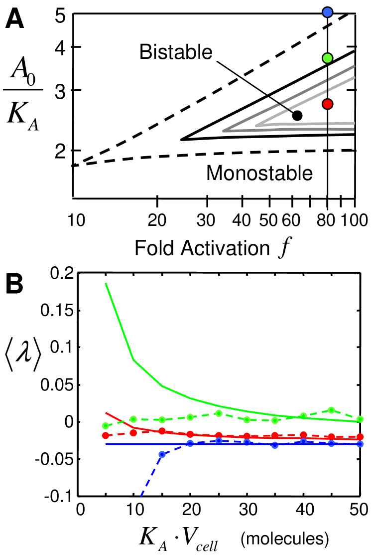
Figure 4: Accuracy of the effective stability approximation (ESA) as a function of the number of molecules. (A) Focusing upon three points in the parameter space of the autoactivator model (see Figure 2a in the main text), it is possible to compare the ESA with the results of numerical simulation. (B) The short-time Lyapunov exponent of an ensemble average of the perturbation modes about the LOW state (dashed lines) approach those values of $\lambda^{\prime}$ predicted according to Eq. 25 (solid lines) for systems with increasing values of $K_{A}\cdot V_{cell}$, which specifies the order of molecule numbers to turn on/off the gene. Here, the burstiness of protein synthesis is held constant at $b=9$, and each data point is computed from a sample of $10^{5}$ trajectories – colors of the curves correspond to the filled circles in panel A.

To compute the accuracy of the effective stability approximation as a function of the molecule numbers for the translational autoactivator model, the corrected eigenvalue $\lambda^{\prime}$ computed above (Eq. 42) is compared to the short-time Lyapunov exponent of the ensemble-averaged perturbation modes computed by stochastic simulation Gillespie (1977).

For a system slightly perturbed from the steady-state $x_{s}$, the short-time Lyapunov exponent $\langle\lambda\rangle$ is defined as,

$$\mathop{\lim}\limits_{t\to 0}\ln\left|{\left\langle{x_{p}\left(t\right)}\right\rangle-x_{s}}\right|=\mbox{const.}+\left\langle\lambda\right\rangle\cdot t.$$

A numerical calculation of $\langle\lambda\rangle$ is obtained by taking the ensemble average (over an ensemble of $10^{5}$ members) of $x_{p}(t)$ determined by stochastic simulation. The slope of the natural-log difference between the numerically generated perturbation mode and the steady state, $\ln|\langle x_{p}(t)\rangle-x_{s}|$, is fit by linear regression over a time span corresponding to the protein lifetime (i.e. $\delta^{-1}=30$ minutes). To compare the stochastic simulation with the ESA, we focus upon three points in the parameter space of the autoactivator (Figure 1a, filled circles) – one point well inside the bistable regime ($\frac{A_{0}}{K_{A}}=2.5,f=80$; red), one near the boundary predicted by the ESA ($\frac{A_{0}}{K_{A}}=3.5,f=80$; green), and one well inside the monostable regime ($\frac{A_{0}}{K_{A}}=5,f=80$; blue). Figure 1b compares the resulting Lyapunov exponent $\langle\lambda\rangle$ (dashed lines) with the ESA prediction $\lambda^{\prime}$ (solid lines), where the line colors correspond to the colors of the filled circles in Figure 1a. Here, the burstiness in protein synthesis is held constant at $b=9$, and the characteristic number of molecules in the system, $K_{A}\cdot V_{cell}$, is increased from 5 to 50. (In the main text, $K_{A}\cdot V_{cell}=25$ so that a burstiness of $b=9$ gives a discreteness parameter of $\Delta_{b_{A}}=\frac{(b+1)}{2}\frac{1}{K_{A}\cdot V_{cell}}=0.2$.) As the number of molecules in the system is increased, the ESA and the numerical simulation results converge. The figure shows the effective stability of the transcriptional autoactivator model is well-characterized by the ESA for systems with $K_{A}\cdot V_{cell}\gtrsim 20$.

VI.1.3 Translational activation

To model the translational activity, we redefine the transcription rate to be constant $\frac{\gamma}{b}$, where $b$ is the maximum burst size at full activation, and allow the activator to control the translation rate through the stoichiometery. We write the synthesis and degradation reactions – in analogy with Eq. 35 above – as,

$$\begin{array}[]{*{20}c}{A\xrightarrow{{\nu_{1}}}A+b\cdot g\left(A\right);}&{\nu_{1}=\frac{{\gamma}}{{b}}},\\ {A\xrightarrow{{\nu_{2}}}A-1;}&{\nu_{2}=\delta\cdot A},\\ \end{array}$$ (45)

where the translational activation affects the stoichiometry through the synthesis step-size $b\cdot g(A)$. Notice that the deterministic equation $\frac{dA}{dt}={\bf S}\cdot{\bm{\nu}}=A_{0}\;g(A)-A$ is identical to the deterministic equation for the transcriptional autoactivator in the previous section. Nonetheless, the change in synthesis stoichiometry from $b\mapsto b\cdot g\left(A\right)$ has a noticeable effect on the resulting stability. As above, we calculate the effective eigenvalue,

$$\lambda^{\prime}=\lambda\left\{{1-\frac{{\left({b\cdot g\left(A^{\star}\right)+1}\right)}}{2}\frac{1}{{V_{cell}\cdot K_{A}}}\cdot h\left({\frac{{A_{0}}}{{K_{A}}},g\left({A^{\star}}\right)}\right)}\right\},$$

where $h(\;\cdot\;)$ is as in Eq. 42. The difference from the transcriptional case is that the burst-size itself is attenuated in the LOW state, and the discreteness parameter approaches the minimal value $\Delta_{b}\to 1/(2V_{cell}\cdot K_{A})$, thereby increasing the residence time in the LOW state.

VI.2 Genetic oscillator

The parameters of Vilar et al. Vilar et al. (2002) correspond to the reduced model parameters:

$$\gamma_{A}=25\;nM\;h^{-1},K_{A}=0.5\;nM,f_{A}=10,$$ (46)

$$\gamma_{R}=5\;nM\;h^{-1},K_{R}=1\;nM,f_{R}^{-1}=0,$$

$$\kappa_{C}=2\times 10^{2}\;nM^{-1}\;h^{-1},\mbox{and }\delta_{A}=1\;h^{-1},$$

where, for simplicity, we make the approximation that 1 molecule / $1\mu m^{3}\approx 1\;nM$ and set $V_{cell}=100\mu m^{3}$. Furthermore, the mRNA degradation and translation rates in the original model give an activator burst size of $b_{A}=5$ and a repressor burst size of $b_{R}=10$.

VI.2.1 Details of the stochastic model

The reduced model (Eq. 6 in the main text) is composed of six elementary reactions:

$$\begin{array}[]{*{20}c}{A\to A+b_{A}}&{\nu_{1}=\frac{{\gamma_{A}}}{{b_{A}}}\cdot g\left({\frac{A}{{K_{A}}},f_{A}}\right)}\\ {A\to A-1}&{\nu_{2}=\delta_{A}\cdot A}\\ {\left({A,R,C}\right)\to\left({A-1,R-1,C+1}\right)}&{\nu_{3}=\kappa_{C}\cdot A\cdot R}\\ {R\to R+b_{R}}&{\nu_{4}=\frac{{\gamma_{R}}}{{b_{R}}}\cdot g\left({\frac{A}{{K_{R}}},f_{R}}\right)}\\ {R\to R-1}&{\nu_{5}=\delta_{R}\cdot R}\\ {\left({R,C}\right)\to\left({R+1,C-1}\right)}&{\nu_{6}=\delta_{A}\cdot C}\\ \end{array}$$ (53)

The stoichiometry matrix ${\bf S}$ and the propensity vector ${\bm{\nu}}$ are then written as,

$${\bf{S}}=\left[{\begin{array}[]{*{20}c}{b_{A}}&{-1}&{-1}&0&0&0\\ 0&0&{-1}&{b_{R}}&{-1}&1\\ 0&0&1&0&0&{-1}\\ \end{array}}\right],$$ (57)

$$\bm{\nu}=\left[{\begin{array}[]{*{20}c}{\frac{{\gamma_{A}}}{{b_{A}}}\cdot g\left({\frac{A}{{K_{A}}},f_{A}}\right)}\\ {\delta_{A}\cdot A}\\ {\kappa_{C}\cdot A\cdot R}\\ {\frac{{\gamma_{R}}}{{b_{R}}}\cdot g\left({\frac{A}{{K_{R}}},f_{R}}\right)}\\ {\delta_{R}\cdot R}\\ {\delta_{A}\cdot C}\\ \end{array}}\right].$$ (64)

Identification of dimensionless parameters in the deterministic model comes from considering the rate equations,

$$\frac{d}{{dt}}\left[{\begin{array}[]{*{20}c}A\\ R\\ C\\ \end{array}}\right]={\bf{S}}\cdot\bm{\nu}=$$ (68)

$$\left[{\begin{array}[]{*{20}c}{\gamma_{A}\cdot g\left({\frac{A}{{K_{A}}},f_{A}}\right)-\delta_{A}\cdot A-\kappa_{C}\cdot A\cdot R}\\ {\gamma_{R}\cdot g\left({\frac{A}{{K_{R}}},f_{R}}\right)-\delta_{R}\cdot R-\kappa_{C}\cdot A\cdot R+\delta_{A}\cdot C}\\ {\kappa_{C}\cdot A\cdot R-\delta_{A}\cdot C}\\ \end{array}}\right].$$ (72)

In what follows, it will be convenient to call $\gamma=\frac{\gamma_{R}}{\gamma_{A}}$ and $A_{0}=\frac{\gamma_{A}}{\delta_{A}}$. Scaling the concentrations with respect to the characteristic concentration $A_{0}$ (i.e. $A=A^{\prime}\cdot A_{0}$, etc.) and time with respect to the activator lifetime, $t=t^{\prime}\cdot\delta_{A}$, the rate equations become,

$$\frac{d}{{dt^{\prime}}}\left[{\begin{array}[]{*{20}c}A^{\prime}\\ R^{\prime}\\ C^{\prime}\\ \end{array}}\right]=$$ (76)

$$\left[{\begin{array}[]{*{20}c}{g\left({A^{\prime}\frac{{A_{0}}}{{K_{A}}},f_{A}}\right)-A^{\prime}-\left[{\frac{{\kappa_{C}\cdot A_{0}}}{{\delta_{A}}}}\right]\cdot A^{\prime}\cdot R^{\prime}}\\ {\gamma\cdot g\left({A^{\prime}\frac{{A_{0}}}{{K_{R}}},f_{R}}\right)-\left[{\frac{{\delta_{R}}}{{\delta_{A}}}}\right]\cdot R^{\prime}-\left[{\frac{{\kappa_{C}\cdot A_{0}}}{{\delta_{A}}}}\right]\cdot A^{\prime}\cdot R^{\prime}+C^{\prime}}\\ {\left[{\frac{{\kappa_{C}\cdot A_{0}}}{{\delta_{A}}}}\right]\cdot A^{\prime}\cdot R^{\prime}-C^{\prime}}\\ \end{array}}\right].$$ (80)

The two additional dimensionless constants are the scaled rate of dimerization $\kappa=\frac{{\kappa_{C}\cdot A_{0}}}{{\delta_{A}}}$ and the ratio of the repressor and activator degradation rates $\epsilon=\frac{{\delta_{R}}}{{\delta_{A}}}$. Henceforth, the primes denoting the dimensionless quantities will be dropped.

Since the variance in the fluctuations is found from the auxiliary matrices ${\bf\Gamma}$ and ${\bf D}$ (cf. Eq. 24), and ${\bf\Gamma}$ is the Jacobian of the deterministic system, the dimensionless stochastic parameters are most easily found by considering ${\bf D}={\bf S}\cdot\mbox{diag}\left[{\bm{\nu}}\right]\cdot{\bf S}^{T}$, ${\bf D}=\left[{{\begin{array}[]{*{20}c}{b_{A}\cdot\gamma_{A}\cdot g_{A}+\delta_{A}\cdot A+\gamma_{C}\cdot A\cdot C}&{\gamma_{C}\cdot A\cdot C}&{-\gamma_{C}\cdot A\cdot C}\\ {\gamma_{C}\cdot A\cdot C}&{b_{R}\cdot\gamma_{R}\cdot g_{R}+\delta_{R}\cdot R+\gamma_{C}\cdot A\cdot C+\delta_{A}\cdot C}&{-\gamma_{C}\cdot A\cdot C-\delta_{A}\cdot C}\\ {-\gamma_{C}\cdot A\cdot C}&{-\gamma_{C}\cdot A\cdot C-\delta_{A}\cdot C}&{\gamma_{C}\cdot A\cdot C+\delta_{A}\cdot C}\\ \end{array}}}\right],$ where $g_{i}\equiv g\left({\frac{A}{{K_{i}}},f_{i}}\right)$. As above, we scale the concentrations with respect to $A_{0}$ and divide through by $\delta_{A}$. Evaluating ${\bf D}$ at the steady-state $\left({A^{\star},R^{\star},C^{\star}}\right)$, where $\frac{{dA}}{{dt}}=\frac{{dR}}{{dt}}=\frac{{dC}}{{dt}}=0$, provides the additional simplifications derived from the rate equations above, written in dimensionless form,

$$g_{A} = A^{\star}+\kappa\cdot A^{\star}\cdot R^{\star},$$ (81)

$$\gamma\cdot g_{R}+C^{\star} = \epsilon\cdot R^{\star}+\kappa\cdot A^{\star}\cdot R^{\star},$$

$$C^{\star} = \kappa\cdot A^{\star}\cdot R^{\star}.$$

Hence, the matrix ${\bf D}$ is written in terms of reactant numbers as,

$$\frac{{\bf{D}}}{{\gamma\cdot A_{0}}}=\left[{\begin{array}[]{*{20}c}{2\left[{\frac{{\left({b_{A}+1}\right)}}{2}}\right]\frac{{g_{A}}}{\gamma}}&{C^{\star}}&{-C^{\star}}\\ {C^{\star}}&{2\left[{\frac{{\left({b_{R}+1}\right)}}{2}}\right]g_{R}+2C^{\star}}&{-2C^{\star}}\\ {-C^{\star}}&{-2C^{\star}}&{2C^{\star}}\\ \end{array}}\right].$$ (85)

Comparing each diagonal element with the characteristic mean reactant number of that species $(N_{A}\sim K_{A}\;V_{cell}$, $N_{R}\sim K_{R}\;V_{cell})$, and ignoring parameters coming from the deterministic model ($g_{A},g_{R},\mbox{and }\gamma$), we have three additional constants - the discreteness in the activator number $\Delta_{b_{A}}=\frac{{\left({b_{A}+1}\right)}}{2}\frac{1}{{K_{A}\cdot V_{cell}}}$, the discreteness in the repressor number $\Delta_{b_{R}}=\frac{{\left({b_{R}+1}\right)}}{2}\frac{1}{{K_{R}\cdot V_{cell}}}$ and the extent of dimerization $\frac{{C^{\star}}}{{K_{R}\cdot V_{cell}}}$. In the main text, we focus upon the effect of varying the deterministic parameter $\epsilon$ and the stochastic parameter $\Delta_{b_{A}}$.

VII Algorithmic Implementation of the the Effective Stability Approximation

The corrections to the deterministic eigenvalues are computed by solving the resolvent equation for the the effective eigenvalues $\lambda^{\prime}$,

$$\mbox{det}[{\lambda^{\prime}\cdot{\bf I}-{\bf J}^{(0)}-\frac{1}{V_{cell}}\hat{\bf J}_{c}(\lambda^{\prime})}],$$ (86)

(Eq. 12 in the main text). In this section, we provide a step-by-step algorithm to form the matrices ${\bf J}^{(0)}$ and $\hat{\bf J}_{c}(\lambda^{\prime})$ from the deterministic reaction rates. In the following, the deterministic state vector is denoted by x and ${\bm{\alpha}}$ denotes the fluctuations in each of the components of ${\bf x}$ (c.f. Section I-C above). The first three steps of the algorithm come from the paper by Elf and Ehrenberg Elf and Ehrenberg (2003).

1. Write the various reactions in terms of their propensity and stoichiometry. The deterministic reaction rates are formed by the product ${\bf S}\cdot{\bm{\nu}}$ (cf. Eqs. 31 and 41 above).

2. From ${\bf S}$ and ${\bm{\nu}}$, construct the matrices ${\bf\Gamma}$ and ${\bf D}$,

   $${\bf\Gamma}_{ij}({\bf x})=\frac{\partial[{{\bf S}\cdot{\bm{\nu}}}]_{i}}{\partial x_{j}}\quad\quad{\bf D}({\bf x})={\bf S}\cdot\mbox{diag}[{\bm{\nu}}]\cdot{\bf S}^{T}.$$ (87)

3. Compute the steady-state covariance in the fluctuations $\bm{\alpha}$ by solving the fluctuation-dissipation relation for each of the entries in the symmetric covariance matrix ${\bf\Xi}$ (where $\Xi_{ij}=\Xi_{ji}=\langle{\alpha_{i}\;\alpha_{j}}\rangle$),

   $${\bf\Gamma}({\bf x}_{s})\cdot{\bf\Xi}+{\bf\Xi}\cdot{\bf\Gamma}^{T}({\bf x}_{s})+{\bf D}({\bf x}_{s})={\bf 0}.$$ (88)

   The steady-states ${\bf x}_{s}$ are calculated from the deterministic reaction rates by solving the algebraic equations $([{{\bf S}\cdot{\bm{\nu}}}]_{{\bf x}={\bf x}_{s}})={\bf 0}$.

   Evaluated at the steady-state, the fluctuation-dissipation relation is simply a $\frac{1}{2}d(d+1)$ system of linear equations that determine the symmetric entries of ${\bf\Xi}$ (where $d$ is the dimension of the system). For more details regarding the general solution of the fluctuation-dissipation relation, see Tomioka et al. (2004).

4. Compute the matrices ${\bf J}^{(0)}$ and ${\bf J}^{(1)}(t)$,

   $${\bf J}^{(0)}={\bf\Gamma}({\bf x}_{s})\quad\quad{\bf J}^{(1)}(t)=\frac{\partial{\bf\Gamma}({\bf x}_{s}+\omega\;{\bm{\alpha}}(t))}{\partial\omega}|_{\omega=0}.$$ (89)

5. Calculate the matrix ${\bf J}_{c}(t)$,

   $${\bf J}_{c}(t)=\langle{{\bf J}^{(1)}(t)\cdot\mbox{exp}[{{\bf J}^{(0)}\;t}]\cdot{\bf J}^{(1)}(0)}\rangle,$$ (90)

   where $\mbox{exp}[{{\bf J}^{(0)}t}]$ is the matrix exponential of ${\bf J}^{(0)}$. The matrix ${\bf J}_{c}(t)$ will be composed of linear combinations of the autocorrelation functions $\langle{\alpha_{i}(t)\;\alpha_{j}(0)}\rangle$. Replace each of these by the ${(i,j)}^{th}$ element of the matrix $\mbox{exp}[{{\bf J}^{(0)}\;t}]\cdot{\bf\Xi}$,

   $$\langle{\alpha_{i}(t)\;\alpha_{j}(0)}\rangle=[{\;\mbox{exp}[{\bf J}^{(0)}\;t]\cdot{\bf\Xi}\;}]_{ij},$$ (91)

   (cf. Eq. 25 above).

6. The correction matrix ${\bf J}_{c}(t)$ is composed of exponential terms of the form $e^{at}$, facilitating the computation of the Laplace transform $\hat{\bf J}_{c}(\lambda^{\prime})$. Simply replace each term $e^{at}$ with $(\lambda^{\prime}-a)^{-1}$,

   $$\hat{\bf J}_{c}(\lambda^{\prime})={\bf J}_{c}(t)|_{e^{at}\to(\lambda^{\prime}-a)^{-1}}.$$ (92)

7. Solve the resolvent equation for $\lambda^{\prime}$,

   $$\mbox{det}[{\lambda^{\prime}\cdot{\bf I}-{\bf J}^{(0)}-\frac{1}{V_{cell}}\hat{\bf J}_{c}(\lambda^{\prime})}].$$ (93)

The algorithm described above is easily implemented in symbolic mathematics packages. A version coded in Mathematica is available from the authors upon request.

References

- Kobiler et al. (2005) O. Kobiler, A. Rokney, N. Friedman, D. L. Court, J. Stavans, and A. B. Oppenheim, Proceedings of the National Academy of Science U.S.A. 102, 4470 (2005).
- Hasty et al. (2002) J. Hasty, D. McMillen, and J. J. Collins, Nature 420, 224 (2002).
- Kaern et al. (2003) M. Kaern, W. J. Blake, and J. J. Collins, Annual Review of Biomedical Engineering 5, 179 (2003).
- Bintu et al. (2005) L. Bintu, N. E. Buchler, H. G. Garcia, U. Gerland, T. Hwa, J. Kondev, and R. Phillips, Current Opinion in Genetics and Development 15, 116 (2005).
- Gillespie (1977) D. T. Gillespie, Journal of Physical Chemistry 81, 2340 (1977).
- Strogatz (1994) S. H. Strogatz, Nonlinear dynamics and chaos (Westview-Perseus, 1994).
- Kaern et al. (2005) M. Kaern, T. C. Elston, W. J. Blake, and J. J. Collins, Nature Reviews Genetics 6, 451 (2005).
- Swain et al. (2002) P. S. Swain, M. B. Elowitz, and E. D. Siggia, Proceedings of the National Academy of Science U.S.A. 99, 12795 (2002).
- van Kampen (1992) N. G. van Kampen, Stochastic Processes in Physics and Chemistry (North-Holland-Elsevier, 1992), chapter VII.
- Aurell and Sneppen (2002) E. Aurell and K. Sneppen, Physical Review Letters 88, 048101 (2002).
- Walczak et al. (2005) A. M. Walczak, J. N. Onuchic, and P. G. Wolynes, Proceeds of the National Academy of Science USA 102, 18926 (2005).
- Vilar et al. (2002) J. M. G. Vilar, H. Y. Kueh, N. Barkai, and S. Leibler, Proceedings of the National Academy of Science U.S.A. 99, 5988 (2002).
- Steuer et al. (2003) R. Steuer, C. Zhou, and J. Kurths, BioSystems 72, 241 (2003).
- Suel et al. (2006) G. M. Suel, J. Garcia-Ojalvo, L. M. Liberman, and M. Elowitz, Nature 440, 545 (2006).
- van Kampen (1976a) N. G. van Kampen, Advances in Chemical Physics 34, 245 (1976a).
- Tanase-Nicola et al. (2006) S. Tanase-Nicola, P. B. Warren, and P. R. ten Wolde, Physical Review Letters 97, 068102 (2006).
- Pedraza and van Oudenaarden (2005) J. M. Pedraza and A. van Oudenaarden, Science 307, 1965 (2005).
- Tomioka et al. (2004) R. Tomioka, H. Kimura, T. J. Kobayashi, and K. Aihara, Journal of Theoretical Biology 229, 501 (2004).
- Paulsson et al. (2000) J. Paulsson, O. G. Berg, and M. Ehrenberg, Proceedings of the National Academy of Science U.S.A. 97, 7148 (2000).
- DeVille et al. (2006) R. E. L. DeVille, C. B. Muratov, and E. Vanden-Eijnden, Journal of Chemical Physics 124, art. 231102 (2006).
- Elf and Ehrenberg (2003) J. Elf and M. Ehrenberg, Genome Research 13, 2475 (2003).
- Isaacs et al. (2003) F. J. Isaacs, J. Hasty, C. R. Cantor, and J. J. Collins, Proceedings of the National Academy of Science U.S.A. 100, 7714 (2003).
- Atkinson et al. (2003) M. R. Atkinson, M. A. Savageau, J. T. Myers, and A. J. Ninfa, Cell 113, 597 (2003).
- J. E. Ferrell (2002) J. J. E. Ferrell, Current Opinion in Cell Biology 14, 140 (2002).
- Keller (1995) A. D. Keller, Journal of Theoretical Biology 172, 169 (1995).
- Thattai and van Oudenaarden (2001) M. Thattai and A. van Oudenaarden, Proceedings of the National Academy of Science U.S.A. 98, 8614 (2001).
- Ozbudak et al. (2002) E. M. Ozbudak, M. Thattai, I. Kurtser, A. D. Grossman, and A. van Oudenaarden, Nature Genetics 31, 69 (2002).
- Kennell and Riezman (1977) D. Kennell and H. Riezman, Journal of Molecular Biology 114, 1 (1977).
- Cai et al. (2006) L. Cai, N. Friedman, and X. S. Xie, Nature 440, 358 (2006).
- Gardiner (2004) C. W. Gardiner, Handbook of Stochastic Methods (Springer, 2004), 3rd ed.
- Kepler and Elston (2001) T. B. Kepler and T. C. Elston, Biophysical Journal 81, 3116 (2001).
- Goldbeter (1997) A. Goldbeter, Biochemical Oscillations and Cellular Rhythms: The Molecular Bases of Periodic and Chaotic Behaviour (Cambridge University Press, 1997).
- Pomerening et al. (2005) J. R. Pomerening, S. Y. Kim, and J. J. E. Ferrell, Cell 122, 565 (2005).
- Elowitz and Leibler (2000) M. B. Elowitz and S. Leibler, Nature 403, 335 (2000).
- Dunlap (1999) J. C. Dunlap, Cell 96, 271 (1999).
- Pomerening et al. (2003) J. R. Pomerening, E. D. Sontag, and J. J. E. Ferrell, Nature Cell Biology 5, 346 (2003).
- Cross and Siggia (2005) F. R. Cross and E. Siggia, Developmental Cell 9, 309 (2005).
- Guantes and Poyatos (2006) R. Guantes and J. F. Poyatos, PLoS Computational Biology 2, 188 (2006).
- Conrad and Tyson (2006) E. D. Conrad and J. J. Tyson, in System modeling in cellular biology (MIT Press, 2006), chap. 6, pp. 97–123.
- Kaern and Weiss (2006) M. Kaern and R. Weiss, in System modeling in cellular biology (MIT Press, 2006), chap. 13, pp. 269–295.
- Ali and Menzinger (1999) F. Ali and M. Menzinger, Chaos 9, 348 (1999).
- Scott et al. (2006) M. Scott, B. Ingalls, and M. Kaern, Chaos 16, art. 026107 (2006).
- Bourret (1965) R. C. Bourret, Canadian Journal of Physics 43, 619 (1965).
- van Kampen (1976b) N. G. van Kampen, Physics Reports 24, 171 (1976b).
- Grossman and Miller (1973) S. I. Grossman and R. K. Miller, Journal of Differential Equations 10, 485 (1973).
- Horsthemke and Lefever (1984) W. Horsthemke and R. Lefever, Noise-induced transitions (Springer, 1984).
- Kerszberg (2004) M. Kerszberg, Current Opinion in Genetics and Development 14, 440 (2004).
- Trefethen and Embree (2005) L. N. Trefethen and M. Embree, Spectra and Pseudospectra : The Behavior of Nonnormal Matrices and Operators (Princeton University Press, 2005).
- van Kampen (1981) N. G. van Kampen, Journal of Statistical Physics 24, 175 (1981).
- Bourret (1962) R. C. Bourret, Nuovo Cimento 26, 1 (1962).
- Miller (1971) R. K. Miller, Journal of Differential Equations 8, 457 (1971).
- McQuarrie (1967) D. McQuarrie, Journal of Applied Probability 4, 413 (1967).
- Kubo et al. (1973) R. Kubo, K. Matsuo, and K. Kitahara, Journal of Statistical Physics 9, 51 (1973).
- Gillespie (2000) D. T. Gillespie, Journal of Chemical Physics 113, 297 (2000).
- Risken (1989) H. Risken, The Fokker-Planck Equation: Methods of Solution and Applications (Springer, Berlin, 1989).