Enhanced activity of massive black holes by stellar capture assisted by a self-gravitating accretion disc

Abstract

Aims. We study the probability of close encounters between stars from a nuclear cluster and a massive black hole ($10^{4}M_{\sun}\lesssim M_{\bullet}\lesssim 10^{8}M_{\sun}$). The gravitational field of the system is dominated by the black hole in its sphere of influence. It is further modified by the cluster mean field (a spherical term) and a gaseous disc/torus (an axially symmetric term) causing a secular evolution of stellar orbits via Kozai oscillations. Intermittent phases of large eccentricity increase the chance that stars become damaged inside the tidal radius of the central hole. Such events can produce debris and lead to recurring episodes of enhanced accretion activity.

Methods. We introduce an effective loss cone and associate it with tidal disruptions during the high-eccentricity phases of the Kozai cycle. By numerical integration of the trajectories forming the boundary of the loss cone we determine its shape and volume. We also include the effect of relativistic advance of pericentre.

Results. The potential of the disc has the efffect of enlarging the loss cone and, therefore, the predicted number of tidally disrupted stars should grow by factor of $\simeq 10^{2}$. On the other hand, the effect of the cluster mean potential together with the relativistic pericentre advance act against the eccentricity oscillations. In the end we expect the tidal disruption events to be approximately ten times more frequent in comparison with the model in which the three effects – the cluster mean field, the relativistic pericentre advance, and the Kozai mechanism – are all ignored. The competition of different influences suppresses the predicted star disruption rate as the black hole mass increases. Hence, the process under consideration is more important for intermediate-mass black holes, $M_{\bullet}\simeq 10^{4}M_{\sun}$.

1 Introduction

According to the present-day consensus, the observational evidence shows black holes populating the mass spectrum in two distinct intervals: stellar-mass black holes, $3M_{\sun}\lesssim M_{\bullet}\lesssim 20M_{\sun}$, that originate from collapse of massive stars and are revealed as members of binary systems; and supermassive black holes (SMBHs; $10^{6}M_{\sun}\lesssim M_{\bullet}\lesssim 10^{9}M_{\sun}$) hosted in nuclei of many galaxies including our own. The existence of intermediate-mass black holes (IMBHs; $10^{2}M_{\sun}\lesssim M_{\bullet}\lesssim 10^{5}M_{\sun}$) is an open issue, likewise their observational consequences and the form of the mass spectrum that might be filling the gap between the two well-established categories of black holes.

Over the last four decades, a picture of galactic nuclei has emerged in which black holes are embedded in a dense stellar system and their masses are increasing by accretion of gas from an accretion disc, gradually inflowing towards the horizon (Begelman & Rees begelman78 (1978); Volonteri & Rees volonteri05 (2005)). Remnants of stars tidally disrupted near a SMBH also contribute as a source of material (Zhao et al. zhao02 (2002)). Previously we demonstrated (Vokrouhlický & Karas vokrouhlicky98 (1998); Šubr et al. subr04 (2004)) that stars of the nuclear cluster can undergo episodes of very large orbital eccentricity if they interact with a self-gravitating disc near a SMBH. This mechanism sets stars on very elongated trajectories with small periapses, although the overall tendency of the gas-assisted drag acts in the opposite way – towards the orbital circularization (Syer et al. syer91 (1991); Vokrouhlický & Karas vokrouhlicky93 (1998)).

In this paper we study the fraction of stars that are set to highly eccentric orbits as a function of the black hole mass. We suggest this problem is relevant in the context of coexistence of a massive black hole with a surrounding cluster of stars. Exactly because of large elongation of the orbits, the fate of the remnant gas from the tidally disrupted stars is very uncertain and we do not attempt to solve this problem in its entirety. Instead, we concentrate our attention on a single aspect – the mutual gravitational interaction of stars and the gaseous disc. Our model is axially symmetric. We study how Kozai’s phenomenon modifies and enlarges the black-hole loss cone and how this change depends on $M_{\bullet}$. We do take several subtleties of this scenario into consideration, namely the damping effect of the star cluster and the relativistic pericentre advance of stellar orbits near the central black hole. These effects pose a potential threat to our mechanism.

We find that a self-gravitating disc is capable of pushing more stars towards less massive (i.e. less-than-supermassive) black holes. Therefore, the effect should be particularly relevant for intermediate-mass black holes, provided they exist embedded within dense stellar systems and accrete from a gaseous disc or a torus (Madau & Rees madau01 (2005); Miller & Hamilton miller02 (2002)).

There is a secondary motivation for our investigation: because the efficiency of the mechanism discussed herein decreases with the black hole mass increasing (it seems to be overwhelmed entirely by damping effects above $M_{\bullet}\sim 10^{7}M_{\sun}$), the present model may be particularly relevant for an ongoing debate about the origin of ultra-luminous X-ray sources (ULXs) and their putative connection with IMBHs (for reviews, see van der Marel marel04 (2003); Fabbiano fabbiano06 (2006)).

ULXs are extra-nuclear point-like X-ray sources with isotropic luminosities exceeding $10^{39}\,\mbox{erg\,s}^{-1}$. It has been proposed (Colbert & Mushotzky colbert99 (1999); Makishima et al. makishima00 (2000); Matsumoto et al. matsumoto01 (2001); Portegies Zwart et al. zwart04 (2004); Hopman et al. hopman04 (2004); Baumgardt et al. baumgardt06 (2006)) that some of them may harbour accreting IMBHs. Within the intermediate black-hole mass range the proposed mechanism is relatively efficient, and we can thus speculate that these ULXs might be triggered when a star is damaged near the tidal radius. This concept seems to be in line also with the idea that accreting pre-galactic seed holes may could indeed be detectable as ULXs (Madau & Rees madau01 (2005)). Also, it appears to be in accord with the manifestation of a multi-colour disc component, as reported in spectra of a sample of ULXs (Miller et al. miller04 (2004); miller06 (2006); Fabian et al. fabian04 (2004)), and it also agrees with indications that ULXs are transient (Miniutti et al. miniutti06 (2006)), possibly recurring phenomenon and that they are switched on during phases of active accretion (see Krolik krolik04 (2004)). However, the evidence for IMBHs is only circumstantial – numerous uncertainties persist in the mass estimates (see the discussion in King et al. king01 (2001); Gonçalves & Soria goncalves06 (2006)), and so our scheme is a mere speculation at this stage.

2 Model and method

2.1 Basic equations

We assume that some kind of an accretion disc surrounds the central black hole and defines the equatorial plane of the system. The presence of the black hole provides a natural length-scale which we will use hereafter: $R_{\mathrm{g}}\equiv{GM_{\bullet}}c^{-2}\simeq 1.5\times 10^{9}M_{4}$ cm, $M_{4}\,\equiv\,M_{\bullet}/(10^{4}M_{\sun})$. The disc is taken as axially symmetric and relatively light with respect to the central black hole ($\mu\equiv M_{\mathrm{d}}/M_{\bullet}\ll 1$). Nevertheless, it is important that $\mu$ is greater than zero. To be specific, we consider two examples: (i) a constant surface density disc, characterized by its mass $M_{\mathrm{d}}$ and the outer radius $R_{\mathrm{d}}$, and (ii) a limiting case of an infinitesimally narrow ring of mass $M_{\mathrm{d}}$ and radius $R_{\mathrm{d}}$. The two cases serve as a useful test-bed because analytical expressions can be derived for the perturbation potential, $V_{\mathrm{d}}(R,z)$, and its first derivatives (Lass & Blitzer lb83 (1983); Huré & Pierens hure05 (2005)). Notice also that the massive ring surrounding the central black hole can represent a time-averaged system with a secondary black hole, sometime invoked in the framework of the hierarchical SMBH formation in centres of merging protogalaxies (Volonteri et al. volonteri03 (2003); Gültekin et al. gultekin04 (2004)). Recently, Ivanov et al. (ivanov05 (2005)) applied the averaging technique to study tidal disruptions of stars in a galaxy centre containing a supermassive binary black hole. However, these authors neglected relativistic effects, which exhibit growing importance near the black hole.

The central cluster is bound gravitationally to the black hole and characterized by distribution function on the space of osculating elements, $D_{\mathrm{f}}(a,C_{1},e,\omega)$, where $C_{1}=\eta\cos i\,$ is a normalized $z$-component of the angular momentum, $\eta\,\equiv\,(1-e^{2})^{1/2}$; $e$ is eccentricity, $a$ is semimajor axis and $\omega$ is argument of pericentre. The orbit inclination $i$ is measured with respect to the disc plane. We consider distribution of the form

$$D_{\mathrm{f}}(a,C_{1},e,\omega)=Ka^{1/4}e\eta^{-1}$$ (1)

with $K$ being a normalization constant. Eq. (1) represents the Bahcall & Wolf (bahcall76 (1976)) distribution with a random orientation in inclinations and linear distribution in eccentricities. The stellar cluster introduces a spherically symmetric perturbation to the central potential, $V_{\mathrm{c}}(r)\propto r^{1/4}$.

Length-scales of the model can be related to the mass according to the empirical relation $M_{\bullet}(\sigma)$ (Tremaine et al. Tremaine02 (2002)) which we extrapolate in a naive way from galactic nuclei down to IMBHs range: $M_{4}\simeq 10^{4}\sigma_{2}^{4}$, where $\sigma_{2}\,\equiv\,\sigma/(200{\rm{}km\,s}^{-1})$ is the velocity dispersion. This seems to be justified by kinematical studies of some globular clusters (e.g., M15, Gerssen et al. gerssen02 (2002); G1, Gebhardt et al. gebhardt05 (2005); 47 Tuc, McLaughlin et al. mclaughlin06 (2006)) and it enables us to introduce the cusp radius,

$$R_{\mathrm{h}}\equiv GM_{\bullet}\sigma^{-2}=2.25\times 10^{8}M_{4}^{-1/2}\!R_{\mathrm{g}}=0.11M_{4}^{1/2}\;\mathrm{pc}\,.$$ (2)

We further assume the mass of the cluster $M_{\mathrm{c}}(R_{\mathrm{h}})\simeq M_{\bullet}$. Finally, we set the disc/ring radius to be equal to the characteristic radius of the cluster: $R_{\mathrm{d}}=R_{\mathrm{h}}$. Thenceforth only $M_{\mathrm{d}}$ is a free parameter.

The axial symmetry of the problem does not ensure conservation of the angular momentum; instead, only one of its components is conserved, so that the orbital eccentricity and inclination of the cluster stars can secularly evolve and fluctuate. In our model we imagine that Kozai’s phenomenon is responsible for oscillations of the orbital elements on the time-scale of

$$T_{\mathrm{K}}\equiv\frac{\lambda}{2\pi\mu}\left(\frac{R_{\mathrm{d}}}{a}\right)^{3}\!P\simeq 1.6\times 10^{3}M_{4}\,\frac{\lambda}{\mu}\left(\frac{R_{\mathrm{d}}}{a}\right)^{3}\left(\frac{a}{10^{8}R_{\mathrm{g}}}\right)^{3/2}\!\!\mathrm{yr}.$$ (3)

The oscillation period exceeds the orbital period $P(a)$ of each individual star, $T_{\mathrm{K}}\gg P=2\pi\,a^{3/2}/(GM_{\bullet})^{1/2}$, by at least one order of magnitude. Factor $\lambda\simeq 1$ includes additional corrections arising from unaccounted effects.

Precession due to an extended spherically symmetric potential component accelerates the oscillations. For $M_{\mathrm{c}}\gtrsim 0.1M_{\bullet}$ we find the correction term to the cycles of eccentricity oscillations,

$$\lambda\simeq 0.1\left(\frac{M_{\mathrm{c}}}{M_{\bullet}}\right)^{-1/2}.$$ (4)

The period $T_{\mathrm{K}}$ from eqs. (3)–(4) fits well with results of the numerical integration shown in Figure 1, where we evaluate the Kozai cycle period as a function of the mass $M_{\mathrm{c}}$ of the spherical cluster. $T_{\mathrm{K}}$ in terms of orbital period $P$ is determined numerically by integrating the trajectories that reach the tidal radius $R_{\mathrm{t}}$ at the maximum of the eccentricity oscillations, i.e. $T_{\mathrm{K}}$ in Fig. 1 is given by the loss cone boundary trajectories. The dependency indicates that the shape of the loss cone is also modified, and we look to this more in the next section.

Figure 1: Kozai period $T_{\mathrm{K}}$ (solid lines) as a function of mass distributed in the spherical potential of the nuclear cluster. Time is scaled with the corresponding orbital period $P$. Principal parameters of the system are the black hole mass, $M_{4}=10$, and the mass of the ring, $M_{\mathrm{d}}=0.1M_{\bullet}$. Trajectories were characterised by $C_{1}=10^{-3}$ and integrated numerically. Two different values of semi-major axis are given by each curve. Also plotted is the approximation to $T_{\mathrm{K}}$ with the value of $\lambda$ from eq. (4), producing the slope $-1/2$ (dotted lines).

2.2 Loss cone in the presence of Kozai’s process

The elongated trajectories bring stars of the nuclear cluster close to the centre. It is then natural to assume that passages near the black hole are moments important for the evolution of the system – feeding the black hole and triggering the accretion activity, as is commonly described in terms of loss-cone processes (e.g. Frank & Rees frank76 (1976); Magorrian & Tremaine magorrian99 (1999); Merritt & Wang merritt05 (2005)).

A ‘classical’ loss-cone is determined by the process of tidal disruption of stars near the central black hole. Low angular momentum trajectories are relevant because stars following these orbits have their periapses within the black hole tidal radius,

$$R_{\mathrm{t}}=\left(\frac{M_{\bullet}}{M_{\star}}\right)^{1/3}\!R_{\star}\simeq 10^{3}M_{4}^{-2/3}\left(\frac{M_{\star}}{M_{\sun}}\right)^{-1/3}\left(\frac{R_{\star}}{R_{\sun}}\right)\,R_{\mathrm{g}},$$ (5)

where $M_{\star}$ and $R_{\star}$ are the stellar mass and radius. The loss-cone is emptied on a time-scale of $\simeq{P}$ provided the perturbing processes are not strong enough to deflect stars from their orbits.

The above-described situation becomes more complicated when the timescales are modified in the presence of Kozai’s mechanism. An ‘effective’ loss cone can be now associated with the new period $T_{\mathrm{K}}>P(a)$ operating in the system. The loss cone is formed by trajectories in phase space plunging below $r=R_{\mathrm{t}}$ by Kozai’s oscillations. This view of the influence of the process takes into consideration the fact that orbital elements evolve in a systematical manner under Kozai’s mechanism. In other words, eccentricities are pumped up to large values for extended periods of time, which makes the effect distinct from the stochastic nature of gravitational scattering. Furthermore, the loss cone geometry is more complex because of the coupling that exists between the mean eccentricity and inclination of the orbits.

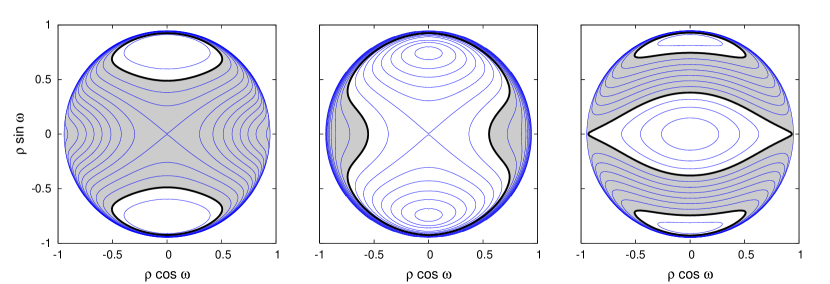
Figure 2: Structure of the orbits is shown in $(\rho,\omega)$ polar plot. To find these orbits, we assume equations of motion in the form (LABEL:eq:eqmotion). For the gravitational field we take different terms into account, so that the effect of perturbations becomes apparent. Always present is the leading term of the Keplerian field (which dominates) and the axisymmetric field $\mbox{\boldmath$\nabla$}V_{\mathrm{d}}$ (which represents the perturbation). In the left panel, no other terms are considered. In the middle panel, the PN1 term of the central field is added. In the right panel, both PN1 of the centre and $\mbox{\boldmath$\nabla$}V_{\mathrm{c}}$ of the cluster are considered. High-eccentricity orbits pass through the shaded regions. Common values of the parameters: $M_{\mathrm{c}}(R_{\mathrm{h}})=M_{\mathrm{d}}=0.01M_{\bullet}$, $R_{\mathrm{d}}=R_{\mathrm{h}}=10^{5}R_{\mathrm{g}}$, $C_{1}=0.1$ and $a=0.4R_{\mathrm{d}}$.

We characterize the influence of highly eccentric orbits on the star capture rate by the fraction of stars that exhibit pericentre distances below a certain threshold radius, $R_{\mathrm{p}}\leq R_{\rm{}min}$. We denote this fraction ${\cal F}_{2}(R_{\rm{}min};a,C_{1})$ and write it in the form

$${\cal F}_{2}\equiv\frac{1}{D_{2}}\int_{0}^{\sqrt{1-C_{1}^{2}}}\!\!\mathrm{d}{e}\!\int_{0}^{2\pi}\!\!\mathrm{d}{\omega}\;\Theta(e_{\mathrm{max}}\!-e_{\mathrm{min}})\;D_{\mathrm{f}}(a,C_{1},e,\omega),$$

where $\Theta$ is the Heaviside step function, $e_{\mathrm{min}}\,\equiv\,1-R_{\rm{}min}/a$, and $e_{\mathrm{max}}(a,C_{1},e,\omega)$ is the maximum eccentricity reached on a given trajectory. The normalization factor is equal to

$$D_{2}(a,C_{1})\equiv\int_{0}^{\sqrt{1-C_{1}^{2}}}\!\mathrm{d}{e}\int_{0}^{2\pi}\!\mathrm{d}{\omega}\;D_{\mathrm{f}}(a,C_{1},e,\omega)\,.$$ (6)

Analogically we define integrated quantities

$${\cal F}_{1}(R_{\rm{}min};a)\equiv\frac{1}{D_{1}(a)}\int_{0}^{1}\mathrm{d}{C_{1}}\;{\cal F}_{2}(R_{\rm{}min};a,C_{1})\,D_{2}(a,C_{1})$$ (7)

and

$${\cal F}(R_{\rm{}min})\equiv\int_{a_{\mathrm{min}}}^{a_{\mathrm{max}}}\mathrm{d}{a}\;{\cal F}_{1}(R_{\rm{}min};a)\,D_{1}(a)\,,$$ (8)

where

$$D_{1}(a)\equiv\int_{0}^{1}\!\mathrm{d}{C_{1}}\;D_{2}(a,C_{1})\,.$$ (9)

The function ${\cal F}(R_{\rm{}min})$ can be interpreted as volume of the loss-cone normalised to the phase space volume occupied by the stellar cluster. (The correspondence between ${\cal F}$ and the volume of the loss cone would be exact in the case of uniform distribution function $D_{\mathrm{f}}$.)

The integrals (2.2)–(9) can be carried out analytically in the Keplerian case. In the non-Keplerian case, however, the function $e_{\mathrm{max}}(a,C_{1},e,\omega)$ is given in an implicit form which complicates the evaluation of the integrals. Our approach is thus based on direct numerical integration of the equations of motion of suitably chosen trajectories, as described below.

2.3 Integration of the orbits

According to the averaging technique (Arnold arnold89 (1989); Brower & Clemence brower61 (1961)) the mean motion is taken over orbital period $P$. This allows us to study the long-term evolution of the osculating parameters, $(e,\omega,a,i)$ in an integrable (Keplerian) potential with a small perturbation. The approach relies on the existence of a third integral of motion (in addition to the energy and $z$-component of the angular momentum) which represents a mean of the perturbing part of the Hamiltonian. The orbital trajectories form a congruence of closed curves in the space of mean eccentricity vs. argument of pericentre.

We use the averaging technique to find parameters of the orbits that reach large eccentricities. Then, for those highly eccentric orbits we integrate the equations of motion directly. Accelerations we take in the form

$$a \!=\! -\frac{GM_{\bullet}}{r^{3}}\mbox{\boldmath$r$}-\frac{GM_{\bullet}}{c^{2}\,r^{3}}\left[v^{2}\mbox{\boldmath$r$}-4(\mbox{\boldmath$r{\cdot}v$})\mbox{\boldmath$v$}-\frac{4GM_{\bullet}}{r}\mbox{\boldmath$r$}\right]-\mbox{\boldmath$\nabla$}(V_{\mathrm{d}}+V_{\mathrm{c}}),$$

assuming that the leading Newtonian term dominates. The bracketed term is the PN1 correction to the gravity of the central mass (see sec. VII of Damour et al. damour91 (1991)), while $V_{\mathrm{d}}$ and $V_{\mathrm{c}}$ represent axially and spherically symmetric perturbations, respectively.

Figure 2 shows a set of tracks of different orbits with their corresponding values of $a$ and $C_{1}$ kept fixed. Pericentre argument $\omega$ stands as the polar angle, whereas $\rho(e)\equiv(1-\eta)^{1/2}$ is the radial coordinate; maximum eccentricity is then on the perimeter of these graphs, $e_{\mathrm{max}}=(1-C_{1}^{2})^{1/2}=0.995$. Two classes of orbits can be distinguished – those which librate around $\omega=\pi/2$ (or $\omega=3\pi/2$) and circulating orbits for which the whole range of $\langle 0,2\pi\rangle$ is allowed. The most eccentric orbits attain their maximum eccentricity $e_{\mathrm{max}}$ at $\cos\omega=0$ in the outer circulating region, as is evident from the plots. Hence, in order to evaluate the fraction ${\cal F}_{2}(R_{\rm{}min};a,C_{1})$ we integrate the orbit evolution starting from $(e,\omega)\,\equiv\,(e_{\mathrm{min}},\pi/2)$. The result of integration determines a boundary of the region occupied by trajectories with the maximum eccentricity $\geq\,e_{\mathrm{min}}$. Topology of the contour plot is crucial for the orbit behaviour.

The shaded area shows an intersection of the loss-cone with the $(a,C_{1})$ plane. In the example of Fig. 2 we set $e_{\mathrm{min}}=0.989$ and highlight the corresponding contour. This defines the boundary of the shaded area within which every orbit reaches $e>e_{\mathrm{min}}$ at some moment of its evolution. In other words, this area contains highly eccentric orbits and it defines the size and the shape of the loss cone. Having the loss-cone boundary defined, we integrate $D_{\mathrm{f}}(a,C_{1},e,\omega)$ over the shaded region and obtain ${\cal F}_{2}(R_{\rm{}min};a,C_{1})$. Finally, we evaluate this function on a grid in the $(a,C_{1})$ space and integrate it numerically to find ${\cal F}_{1}(R_{\rm{}min};a)$ and ${\cal F}(R_{\rm{}min})$.

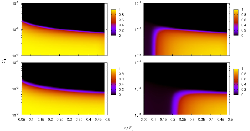
Figure 3: This figure exhibits a clear distinction between the cases with (on the right) and without (on the left) the relativistic pericentre advance taken into account. We draw the fraction ${\cal F}_{2}(R_{\rm{}min};a,C_{1})$ of stars from the ensemble (1) that plunge below $R_{\rm{}min}=100R_{\mathrm{g}}$; $a$ and $C_{1}$ are constants of motion. The central black hole mass $M_{\bullet}=3.6\;10^{6}M_{\sun}$, the disc mass $M_{\mathrm{d}}=0.1M_{\bullet}$. In the bottom panels we assumed the central gravitational field perturbed by a narrow ring. In the upper panels, the case of a constant-density disc was considered. The left column is for the Newtonian potential of the central source, while on the right side we employed the post-Newtonian (PN1) model. Value of ${\cal F}_{2}$ is encoded by a colour palette, ranging from zero to unity. Therefore, this figure demonstrates how sensitive the value of ${\cal F}_{2}$ is with respect to the pericentre precession and the eccentricity oscillations – the two effects which act against each other. Notice a sharp drop of ${\cal F}_{2}$ below a certain critical value of $a=a_{\mathrm{t}}$ (in the panels on the right side). This break emerges once the pericentre advance is taken into account; it does not occur in the left panels because these were computed in purely Newtonian gravity.

The three panels exhibit different possible topologies of the tracks of orbits that arise due to the perturbing forces. In order to construct these plots, the central Keplerian potential was superposed with the perturbation $\mbox{\boldmath$\nabla$}V_{\mathrm{d}}$ (left); with PN1 correction and $\mbox{\boldmath$\nabla$}V_{\mathrm{d}}$ terms added (middle); and with PN1 correction and $\mbox{\boldmath$\nabla$}(V_{\mathrm{d}}+V_{\mathrm{c}})$ terms taken into account (right).

In a conservative system, which is what we consider in Fig. 2, star tracks remain attached to the contours. However, additional dissipative processes might allow adiabatic evolution of the orbital parameters, so that stars can slide gradually across the level surfaces on very long time-scales. This may cause a decay of the orbits and help to bring stars to the centre. We do not consider such effect here, but see Šubr & Karas (subr05 (2005)) where Kozai’s resonance mechanism and the hydrodynamical (dissipative) drag are both taken into account.

3 Results

As mentioned above, Kozai’s resonance mechanism is active when the Newtonian central potential is perturbed by an axisymmetric term – i.e. the disc potential in our case, however, the effect is known to be fragile with respect to various other perturbations that may influence the motion of stars. Namely, it is suppressed when the central field is non-Newtonian, leading to the precession of the orbits. Therefore we want to clarify whether Kozai’s mechanism is still relevant for the long-term dynamics of nuclear stars even if relativistic pericentre advance and the effect of the nuclear cluster are taken into account.

3.1 Fractional probabilities

First we neglect all perturbing terms in the gravitational field and assume purely Keplerian motion. The maximum eccentricity along each trajectory is simply $e_{\mathrm{max}}(a,C_{1},e,\omega)\,\equiv\,e=\mbox{const}$. Assuming the distribution (1), fractional probabilities ${\cal F}_{i}$ can be then written in the explicit form:

$${\cal F}_{2}(R_{\rm{}min};a,C_{1})=\frac{\eta_{\mathrm{min}}-C_{1}}{1-C_{1}}\,\Theta(\eta_{\mathrm{min}}-C_{1})\,,$$ (11)

where $\eta_{\mathrm{min}}\equiv\,(1-e_{\mathrm{min}}^{2})^{1/2}$,

$${\cal F}_{1}(R_{\rm{}min};a)=\eta^{2}_{\mathrm{min}}=\frac{2R_{\rm{}min}}{a}-\frac{R_{\rm{}min}^{2}}{a^{2}}\,,$$ (12)

$${\cal F}(R_{\rm{}min}) = \frac{10\,R_{\rm{}min}\left(a_{\mathrm{max}}^{1/4}-a_{\mathrm{min}}^{1/4}\right)+\frac{5}{3}R_{\rm{}min}^{2}\left(a_{\mathrm{max}}^{-3/4}-a_{\mathrm{min}}^{-3/4}\right)}{a_{\mathrm{max}}^{5/4}-a_{\mathrm{min}}^{5/4}}$$ (13)

$$\simeq 10\,R_{\rm{}min}\,a_{\mathrm{max}}^{-1}\,.$$ (14)

To derive the approximation (14) we assumed $R_{\rm{}min}\ll a_{\mathrm{min}}\ll a_{\mathrm{max}}$.

Under an axially symmetric perturbation of the central potential the total angular momentum of orbits is no longer conserved, nevertheless, its $z$-component remains an integral of motion. This results in oscillations of eccentricity. An upper estimate of the corresponding probabilities can be derived from the loss-cone condition, $L_{z}<L_{\mathrm{max}}$, which can be expressed as $e_{\mathrm{max}}(a,C_{1},e,\omega)=(1-C_{1}^{2})^{-1/2}$. Then,

$${\cal F}_{2}(R_{\rm{}min};a,C_{1})=\Theta(\eta_{\mathrm{min}}-C_{1})\,,$$ (15)

$${\cal F}_{1}(R_{\rm{}min};a)=2\eta_{\mathrm{min}}-\eta_{\mathrm{min}}^{2}\simeq 2\left(2R_{\rm{}min}\,a^{-1}\right)^{1/2}\,,$$ (16)

and

$${\cal F}(R_{\rm{}min})\simeq\frac{10}{3}\frac{\left(2R_{\rm{}min}\right)^{1/2}\left(a_{\mathrm{max}}^{3/4}-a_{\mathrm{min}}^{3/4}\right)}{a_{\mathrm{max}}^{5/4}-a_{\mathrm{min}}^{5/4}}\simeq 4.71\left(\frac{R_{\rm{}min}}{a_{\mathrm{max}}}\right)^{1/2}\!\!.$$ (17)

The last term on the right-hand side gives the values two to three orders of magnitude larger than those which follow from eq. (14). The estimate (17) is good provided the Kozai mechanism is the only one determining the orbital changes. However, this resonance mechanism may be diminished by other perturbations, so the actual value of ${\cal F}(R_{\rm{}min})$ should be somewhere in between the two estimates. We will now discuss the importance of damping effects.

Figure 4: Fraction ${\cal F}_{1}(R_{\mathrm{t}};a)$ of stars plunging below the black hole tidal radius. Stellar orbits are perturbed by a massive ring of radius $R_{\mathrm{d}}$ and mass $M_{\mathrm{d}}=\mu M_{\bullet}$ (indicated with curves). The dashed line is for the PN1 approximation of the central mass gravity field; the effect of the outer stellar cluster is neglected. Solid lines represent two cases in which the cluster is taken into account (they differ by the disc mass parameter $\mu$). Dotted are two power-law lines corresponding to the lower and the upper analytical estimates, eqs. (12) and (16), respectively. Vertical dashed lines indicate the values of $a_{\mathrm{t}}$ (given by eq. (18) with $\mu=0.01$ and $0.1$, respectively); these are critical semiaxis values below which Kozai’s phenomenon is suppressed. For $a>a_{\mathrm{t}}$ the eccentricity oscillations persist. Parameter values assumed in this plot are: in the left panel $M_{\bullet}=10^{4}M_{\sun}$; in the right panel $M_{\bullet}=10^{5}M_{\sun}$.

The relativistic advance of pericentre has an overall tendency of decreasing the maximum eccentricity over the Kozai cycle. Below a certain threshold value of $a$ the maximum eccentricity is not sufficient to bring stars inside the tidal radius; the loss-cone condition is then $L<L_{\mathrm{max}}$. We estimate this terminal value as

$$a_{\mathrm{t}}^{7}\simeq{\textstyle{\frac{32}{9}}}\,R_{\mathrm{d}}^{6}\,R_{\mathrm{g}}^{2}\,R_{\rm{}min}^{-1}\,\mu^{-2}$$ (18)

(see Appendix A). For $a>a_{\mathrm{t}}$ the maximum eccentricity allowed by the relativistic corrections is large enough, so that the pericentre gets below $R_{\mathrm{min}}$. Hence, the fraction of tidally disrupted stars is determined solely by the estimate (12) for $a<a_{\mathrm{t}}$, while above $a_{\mathrm{t}}$ the fraction increases abruptly and saturates almost at the value (16).

3.2 Stars plunging below a threshold radius

In figure 3 we plot the fractional probability ${\cal F}_{2}(R_{\rm{}min};a,C_{1})$, as we obtained it numerically. Comparison between different panels clearly demonstrates the reason for the concern that the pericentre advance of stellar orbits might completely erase the effect of resonance.

One can see that Kozai’s mechanism indeed sets stars on eccentric trajectories reaching small radii and that the efficiency of the process increases with $a$ decreasing down to a certain limiting value. We considered both the Newtonian and the post-Newtonian models of the central field, so the effect of the relativistic pericentre advance can be distinguished. We find that ${\cal F}_{2}$ is raised by a factor of $\simeq 100$ due to the Kozai mechanism and it drops at small semi-axis; the exact value of $a$ where that break occurs depends on the adopted form of the perturbing potential. Comparison of the panels reveals that the disc-like source of the gravity competes more successfully with the relativistic effect than a narrow ring of the same mass.

The mean potential of the extended cluster of stars also causes secular precession of the orbits but this time it alters the results in a different way than the relativistic pericentre advance by attenuating the Kozai oscillations in the whole range of semi-major axes. Nevertheless, it still allows a substantial fraction of orbits to reach high eccentricities.

The fraction ${\cal F}_{1}(R_{\mathrm{t}};a)$ is shown in figure 4. We find the damping effects to be weakened if the mass of the axisymmetric component is higher, as expected. By increasing the mass parameter $\mu$ the curve of ${\cal F}_{1}(R_{\mathrm{t}};a)$ gets gradually shifted to larger values. Simultaneously, $a_{\mathrm{t}}$ is diminished. As consequence of these dependencies, more stars reach the tidal radius for lower mass of the central body than for higher masses. For the sake of definiteness, we assume solar-type stars ($M_{\star}=1M_{\sun}$ and $R_{\star}=1R_{\sun}$) in the evaluation of $R_{\mathrm{t}}$ in eq. (5).

Finally, the overall fraction ${\cal{}F}(R_{\rm{}min})$ is shown in figure 5. The limits on semi-major axes range are set mainly by numerical arguments: the lower limit results from a sharp increase of the Kozai time $T_{\mathrm{K}}$ when $a$ is decreased. Below $a_{\mathrm{min}}=0.04R_{\mathrm{h}}$ the orbits would contribute to the tidal disruption rate only marginally. The upper limit has to be set due to limitations of our approach – at $r\simeq R_{\mathrm{d}}$ the orbits exhibit chaotic motion and they no more follow the curves of figure 2. We assume that these orbits will lead to the disruptions and, therefore, results presented here should be considered as lower estimates.

Line types help us to distinguish the importance of different effects in this plot. In particular:

• Kozai’s oscillations rise the value of $\cal F$ with respect to an unperturbed ($\mu=0$) case;

• PN1 corrections to the central (Keplerian) potential reduce $\cal F$ by factor $\simeq 2\div 5$ (the expected rate of tidal disruptions is diminished accordingly);

• precession due to self-gravity of the cluster decreases $\cal F$ further down by another factor $\simeq 10$.

Figure 5: Fraction ${\cal F}(R_{\rm{}min})$ of stars reaching the pericentre below a given radius $r=R_{\rm{}min}$. We assumed perturbing potentials $V_{\mathrm{d}}(R,z)$ of the disc with constant surface density (top panels) and a narrow ring (bottom panels). Left: the functional dependence of probability ${\cal F}(R_{\rm{}min})$ (solid lines). Parameters compatible with Sgr A^⋆ were assumed: $M_{\bullet}=3.5\times 10^{6}M_{\sun}$, $0.01\leq\mu\leq 0.1$, $R_{\mathrm{h}}\simeq R_{\mathrm{d}}=1.2\times 10^{7}R_{\mathrm{g}}=2$ pc, and $0.04R_{\mathrm{h}}\leq{a}\leq 0.4R_{\mathrm{h}}$. Right: the mass dependence, ${\cal F}(R_{\mathrm{t}}(M_{\bullet}))$, computed according to eqs. (2) and (5). In all panels dotted lines correspond to the analytical estimates (13) and (17); values given by the latter correspond within a factor of $\lesssim 2$ to the case omitting both the relativistic pericentre advance and the stellar cluster reducing of the Kozai oscillations. Dashed lines represent models with only the relativistic precession switched on ($\mu=0.01$), while the solid lines include also the precession from the cluster potential (two cases are shown, $\mu=0.01$ and $0.1$).

As in the previous figures, it is clearly visible that the potential of the extended source, i.e. the disc, competes more successfully against damping than the ring. Increasing the mass of the axial perturbation not only rises $\cal F$ to higher values, but it also changes the slope. That tendency can be attributed to larger terminal value $a_{\mathrm{t}}$ of the semi-major axis, above which the relativistic damping is negligible.

The effect of relativistic pericentre advance increases with the mass of the black hole. The right panels of Fig. 5 demonstrate that ${\cal{}F}$ is anti-correlated with $M_{\bullet}$ and grows towards less massive black holes (i.e. when going from SMBH to IMBH).

4 Discussion

We examined the idea of Kozai’s effect assisted by an accretion disc as the mechanism enhancing the disruption rate of stars by a central black hole. This process is more efficient for intermediate-mass black holes than for supermassive ones. In our calculations we used PN1 approximation of the central field. We performed these calculations also within the pseudo-Newtonian (Paczyński–Wiita paczynski80 (1980)) framework (as a check of the orbits very near horizon) with very similar conclusions.

The results for ${\cal F}(R_{\mathrm{t}})$ can be directly interpreted as fraction of stars populating the loss-cone when an axisymmetric perturbation is applied on the cluster. We suggest that this picture is relevant in a system where gas clouds form an embedded disc-like structure with a non-negligible total mass near the sphere of dominance of a central black hole.

4.1 Disturbing processes

The view presented here is valid as far as other processes, acting on time scales shorter than $T_{\mathrm{K}}$, do not manage to expell the stars from the effective loss cone. This would inhibit the Kozai process. One of the generic processes that may interfere with the influence of the axisymmetric perturbation is the two-body relaxation within the stellar cluster.

Gravitational relaxation brings the diffusion time-scale into the problem, $T_{\theta}\,\equiv\,\theta_{\mathrm{lc}}^{2}T_{\mathrm{r}}$, where

$$\theta_{\mathrm{lc}}=\sqrt{R_{\mathrm{t}}/r}\simeq\sqrt{{\cal F}(R_{\mathrm{t}})}\ll 1$$ (19)

is an angular extent of the loss cone and

$$T_{\mathrm{r}}=\frac{\sigma^{3}}{G^{2}C\ln\Lambda\,M_{\ast}^{2}n_{\ast}}\,.$$ (20)

Here, $n_{\ast}$ is the number density of the stellar system, $\ln\Lambda$ is Coulomb logarithm and $C$ is a constant (in usual notation, $C\ln\Lambda\sim 10^{2}$; Spitzer S87 (1987)). In a cusp described by the Bahcall–Wolf distribution, velocity dispersion is comparable with Keplerian velocity and the number density of stars decreases with radius as $n_{\ast}(r)\propto r^{-7/4}$. Characterizing the number density by the stellar mass $M_{\mathrm{c}}$ enclosed within the radius $R_{\mathrm{h}}$, we get

$$T_{\mathrm{r}}\simeq 10^{6}\,M_{4}^{2}\,\left(\frac{M_{\mathrm{c}}}{M_{\bullet}}\right)^{-1}\left(\frac{M_{\ast}}{M_{\odot}}\right)^{-2}\left(\frac{R_{\mathrm{h}}}{10^{8}R_{\mathrm{g}}}\right)^{5/4}\left(\frac{r}{10^{8}R_{\mathrm{g}}}\right)^{1/4}{\rm yr}\;.$$ (21)

The effective loss cone which we have invoked in Sec. 2.2 generally exceeds $\theta_{\mathrm{lc}}$. From Fig. 5 we see that its volume ${\cal F}(R_{\mathrm{t}})$ is (for $\mu=0.1$ and a ring source of the perturbation) by factor $>10$ larger than it is in an unperturbed system. Hence, appropriate $\theta_{\mathrm{lc}}^{\prime}$ must be by a factor $\gtrsim 3$ larger than $\theta_{\mathrm{lc}}$. However, the geometry of the effective loss cone is more complicated. In particular, it is narrower at $\omega=\pi/2$ where it actually coincides with the boundary of the classical loss cone. Therefore, at $\omega$ corresponding to the minimum eccentricity the new loss cone must be sufficiently wider so that its volume can exceed by a factor of ten the classical one. We estimate $\theta_{\mathrm{lc}}^{\prime}\simeq 10\theta_{\mathrm{lc}}$, which is also in accordance with our experience that the pericentre value on the boundary orbit of the effective loss cone typically changes by more than two orders of magnitude. The time scale on which stars diffuse across the effective loss-cone is then

$$T_{\theta}^{\prime}\simeq 100\,T_{\theta}\simeq 0.04\,M_{4}^{3/2}\left(\frac{M_{\mathrm{c}}}{M_{\bullet}}\right)^{-1}\left(\frac{M_{\ast}}{M_{\odot}}\right)^{-1}\left(\frac{r}{R_{\mathrm{h}}}\right)^{-9/4}P.$$ (22)

By comparing $T_{\mathrm{K}}$ and $T_{\theta}^{\prime}$ we deduce that for $M_{4}\gtrsim 10$ the Kozai mechanism affects the angular momentum on a significantly shorter time-scale and we may consider the effective loss cone to be emptied by this process.

For lower BH masses the interplay of Kozai mechanism and the two-body relaxation is more complicated, however, we still expect that systematic character of the angular momentum changes due to the Kozai mechanism will enhance the rate of tidal disruptions. A definitive study of these systems is probably not possible without employing high precision $N$-body integrators.

We imagine that consumption of stars by the central IMBHs is a transient process which enhances their activity during those periods when stars are supplied into the loss-cone and then efficiently brought onto eccentric orbits. Permanent replenishment of this larger loss cone is not critical for the process considered here. Nevertheless, we may assume that the larger loss cone is replenished more frequently (also by other processes than the steady state relaxation – for example the effect of Brownian motion of the central black hole, or a secondary black hole can contribute). However, details of the loss-cone refilling are beyond the scope of our present paper. It will be interesting to compare these speculations with the results of $N$-body simulations that have been recently applied to explore the tidal processes and their effect on IMBHs formation and feeding in dense star clusters (see Baumgardt et al. baumgardt06 (2006)).

To achieve a more complete description one has to invoke other diffusive processes acting together with the gravitational relaxation (e.g. the hydrodynamical drag by the disc gas that continuously helps re-filling the loss-cone; see e.g. Karas & Šubr karas01 (2001) for relevant time-scales) but, again, this is beyond the scope of our paper.

4.2 Dependence on the black hole mass

Let us consider two types of object which differ from each other by the black hole mass – (i) a supermassive black hole in the Galaxy center, and (ii) hypothetical intermediate-mass black holes that might reside in cores of dense star clusters.

Precise tracking of the proper motion of individual stars is currently possible within an arcsecond area around the Galaxy centre (Genzel et al. genzel03 (2003); Ghez et al. ghez03 (2003)), and so the idea of applying our calculation to Sgr A^⋆ is quite natural and it raises a question about the origin of various perturbations that may act on stellar motion. Currently, $M_{\mathrm{d}}\simeq 0.1M_{\bullet}$ can be set as an upper estimate of the mass of the molecular circumnuclear disc which extends from $\sim 1.5$ pc to $3\div 4$ pc (Christopher et al. christopher05 (2005)), i.e. on the outer edge of the black hole’s sphere of influence. This is compatible with a narrow ring of radius $R_{\mathrm{d}}=R_{\mathrm{h}}\simeq 2\mathrm{pc}$, and so we can directly evaluate the expected number of tidal disruptions. From Fig. 5 we read that the fraction $\simeq 5\times 10^{-4}$ of the total number of stars in the cluster with $a_{\mathrm{max}}<0.4R_{\mathrm{d}}$ exhibit sufficiently large eccentricity oscillations. This corresponds to the mass in stars about $\simeq 0.1M_{\bullet}\simeq 3\times 10^{5}M_{\sun}$, thence we obtain $\simeq 150$ tidal disruption events per $T_{\mathrm{K}}\simeq 10\;\mathrm{Myr}$.

So far we assumed that the source of the gravitational perturbation was a gaseous disc or a torus, however, its origin could be different. In the Sgr A^⋆ there is a disc of young stars (Levin & Beloborodov levin03 (2003); Paumard et al. paumard06 (2006)) and, possibly, a remnant gas from which these stars had been born. To model their effect we consider a thin disc of mass $0.01M_{\bullet}$ and surface density $\propto R^{-2}$ extending between $0.03\div 0.3\;\mathrm{pc}$. We found that $\simeq 2$% of stars from the region $<0.3\mathrm{pc}$ can undergo the oscillations that bring them down to $R_{\mathrm{t}}$. This means that during the period of $T_{\mathrm{K}}\lesssim 1\mathrm{Myr}$ after the formation of the gaseous/stellar disc there may have occurred up to $\simeq 100$ more tidally disrupted stars compared to the result of calculations neglecting the effect. The phase of enhanced disruption rate may become prolonged if the orientation of the disc varies in time. This could be caused by precession in the outer galactic potential.

In the case of IMBHs the resonance mechanism complements the role of stellar encounters in the process of feeding the black hole. If the total mass of the cluster is about $M_{\bullet}\simeq 10^{4}M_{\sun}$, we expect the enhancement of the disruption rate $\simeq 1M_{\sun}$ per $10^{3}$ yrs (with $\mu=0.1$). Disrupted stars then provide material for accretion, thereby triggering a transient luminous phase of the object.

We remark that the model has only formal validity near the lower end of the black-hole mass range because in this case the accretion rate of $\simeq 10^{-3}M_{\bullet}\,\mbox{yr}^{-1}$ is comparable with the mass carried by individual stars; other processes must be important under such circumstances (which is consistent with the expectation that the accretion of stellar material onto IMBH is a non-steady process). Therefore, the scenario outlined above conforms to the assumption that ULXs are a transient phenomenon for which accretion of the surrounding medium is essential.

5 Conclusions

Disruption of stellar bodies and subsequent accretion of the remnant gas are among likely mechanisms feeding black holes that are embedded in a dense cluster. We discussed one of the channels that may contribute to this process. Kozai’s mechanism can enhance the rate of such events, trigger the episodic gas supply onto the black hole, and, consequently, strengthen the activity of the system by raising the accretion rate. The process acts at characteristic time-scale of the Kozai cycle – typically $T_{\mathrm{K}}\simeq 10^{5}$ yrs for IMBHs, during which the loss cone is depleted.

Stars on highly elongated orbits are susceptible to tidal disruption and hence they provide a natural source of material to replenish the inner disc. We have demonstrated that this phenomenon operates in the system even if it is disturbed by the relativistic pericentre precession and gravity of the nuclear cluster. Therefore we can conclude that the presence of a gaseous disc of a small but non-zero mass, $0<M_{\mathrm{d}}<M_{\bullet}$, helps dragging stars to the black hole, thereby feeding the centre and simultaneously providing material that sustains and replenishes the disc itself.

Appendix A The role of GR pericentre advance

Here we want estimate the region of the parameter space where the general relativistic pericentre advance dominates over the Kozai effect. The quadrupole approximation leads to evolutionary equations (Kiseleva et al. kiseleva98 (1998); Blaes et al. blaes02 (2002)):

$$T_{\mathrm{K}}\,\eta\,\,\frac{\mathrm{d}i}{\mathrm{d}t} \!=\! -\frac{15}{8}\,e^{2}\,\sin 2\omega\,\sin i\,\cos i\,,$$ (23)

$$T_{\mathrm{K}}\,\eta\,\,\frac{\mathrm{d}e}{\mathrm{d}t} \!=\! {\frac{15}{8}}\,e\,\eta^{2}\,\sin 2\omega\,\sin^{2}i\,,$$ (24)

$$T_{\mathrm{K}}\,\eta\,\,\frac{\mathrm{d}\omega}{\mathrm{d}t} \!=\! \frac{3}{4}\left\{2\eta^{2}+5\sin^{2}\omega\left[e^{2}-\sin^{2}i\right]\right\}+T_{\mathrm{K}}\,\frac{R_{\mathrm{g}}}{a\,\eta}\,\frac{6\pi}{P}\,.$$ (25)

The last term on the right-hand side of eq. (25) includes the relativistic pericentre advance.

Equations (23)–(25) imply conservation of

$$C_{1}=\eta\,\cos i$$ (26)

and

$$C_{2}=\left(5\sin^{2}i\,\sin^{2}\omega-2\right)\,e^{2}-\frac{8\,R_{\mathrm{d}}^{3}\,R_{\mathrm{g}}}{\mu\,\eta\,a^{4}}\,.$$ (27)

Solutions of two types can be found – circulating vs. librating – depending on the motion constants $a$, $C_{1}$, and $C_{2}$. The circulation region exists always while the libration region occurs typically for small values of $C_{1}$. The two categories are separated by the separatrix curve that passes through $e=0$ point in the plane of $(e,\omega)$ polar coordinates. This can be used to determine the value of $C_{2}$ on the separatrix:

$$C_{2,\mathrm{s}}=-\frac{8R_{\mathrm{d}}^{3}\,R_{\mathrm{g}}}{\mu\,a^{4}}\,.$$ (28)

Maximum eccentricity on the separatrix is given by equation

$$5\left(1-\frac{C_{1}^{2}}{\eta_{\mathrm{s}}^{2}}\right)-\frac{8R_{\mathrm{d}}^{3}\,R_{\mathrm{g}}}{\mu\,a^{4}}\frac{1}{\eta_{\mathrm{s}}(1+\eta_{\mathrm{s}})}=2\,,$$ (29)

which for $\eta_{\mathrm{s}}\ll 1$ simplifies to the form

$$3\eta_{\mathrm{s}}^{2}-\frac{8R_{\mathrm{d}}^{3}\,R_{\mathrm{g}}}{\mu\,a^{4}}\,\eta_{\mathrm{s}}=5C_{1}^{2}.$$ (30)

We are interested in $C_{1}$ small. For $C_{1}\lesssim 0.01$, the circulating solutions cover about half of the $(e,\omega)$ parameter space. These orbits acquire eccentricities larger than $e_{\mathrm{s}}$ at some moment during the orbit evolution. Hence, when $e_{\mathrm{s}}(a,C_{1})>1-a/R_{\rm{}min}$ the fraction ${\cal F}_{2}(R_{\rm{}min};a,C_{1})$ is close to the corresponding estimate (15) which assumes that all orbits with given values of $a$ and $C_{1}$ reach the pericentre below $R_{\rm{}min}$. Setting $\eta_{\mathrm{s}}^{2}=1-e_{\mathrm{min}}^{2}\simeq 2R_{\rm{}min}/a$, eq. (30) gives an implicit formula for the boundary of these two regions in ($a,C_{1}$) plane. We can solve (30) for $C_{1}=0$ to determine the terminal value (18) of semi-major axis $a_{\mathrm{t}}$. Below this value the relativistic pericentre advance inhibits the Kozai mechanism.

References

- (1) Alexander T., 2005, Physics Reports, 419, 65
- (2) Arnold V. I., 1989, Mathematical Methods of Classical Mechanics (Springer-Verlag, Berlin)
- (3) Bahcall J. N., Wolf R. A., 1976, ApJ, 209, 214
- (4) Baumgardt H., Hopman C., Portegies Zwart S., Makino J., 2006, MNRAS, 372, 467
- (5) Begelman M., Rees M. J., 1978, MNRAS, 185, 847
- (6) Blaes O., Lee M. H., Socrates A., 2002, ApJ, 578, 775
- (7) Brower D., Clemence G., 1961, Methods of Celestial Mechanics (Academic Press, New York)
- (8) Christopher M. H., Scoville N.Z., Stolovy S. R., Yun M. S., 2005, ApJ, 622, 346
- (9) Colbert E. J. M., Mushotzky R. F., 1999, ApJ, 519, 8
- (10) Damour T., Soffel M., Xu C., 1991, Phys. Rev. D, 43, 3273
- (11) Fabian A. C., Ross R. R., Miller J. M., 2004, MNRAS, 355, 359
- (12) Fabbiano G., 2006, ARA&A, 44, 323
- (13) Frank J., Rees M. J., 1976, MNRAS, 176, 633
- (14) Gebhardt K., Rich R. M., Ho L. C., 2005, ApJ, 634, 1093
- (15) Genzel R., Schödel R., Ott T., Eisenhauer F. et al., 2003, ApJ, 594, 812
- (16) Gerssen J., van der Marel R. P., Gebhardt K., Guhathakurta P., Peterson R. C., Pryor C., 2002, AJ, 124, 3270
- (17) Ghez A. M., Becklin E. E., Duchêne G., Hornstein S., Morris M., Salim S., Tanner A., 2003, Astron. Nachr., 324, 527
- (18) Gonçalves A. C., Soria M., 2006, MNRAS, 371, 673
- (19) Gültekin K., Miller M. C., Hamilton D. P., 2004, ApJ, 616, 221
- (20) Hopman C., Portegies Zwart S. F., Alexander T., 2004, ApJ, 604, L101
- (21) Huré J.-M., Pierens A., 2005, ApJ, 624, 289
- (22) Ivanov P. B., Polnarev A. G., Saha P., 2005, MNRAS, 358, 1361
- (23) Karas V., Šubr L., 2001, A&A, 386, 686
- (24) King A. R., Davies M. B., Ward M. J., Fabbiano G., Elvis M., 2001, ApJ, 559, L101
- (25) Kiseleva, L. G., Eggleton P. P., Mikkola S., 1998, MNRAS, 300, 292
- (26) Kozai Y., 1962, AJ, 67, 591
- (27) Krolik J. H., 2004, ApJ, 615, 383
- (28) Lass H., Blitzer L., 1983, Celest. Mech. Dyn. Astron., 30, 225
- (29) Levin Y., Beloborodov A. M., 2003, ApJ, 590, L33
- (30) Lidov M. L., 1962, Planetary and Space Sci., 9, 719
- (31) Madau P., Rees M. J., 2001, ApJ, 551, L27
- (32) Magorrian J., Tremaine S., 1999, MNRAS, 309, 447
- (33) Makishima K., Kubota A., Tsunefumi M., Tomohisa O. et al., 2000, ApJ, 553, 632
- (34) Matsumoto H., Tsuru T. G., Koyama K., Awaki H., Canizares C. R., Kawai N., Matsushita S., Kawabe R., 2001, ApJ, 574, L25
- (35) McLaughlin D. E., Anderson J., Meylan G., Gebhardt K., Pryor C., Minniti D., Phinney S., 2006, ApJSS, 166, 249
- (36) Merritt D., Wang J., 2005, ApJ, 621, L101
- (37) Miller M. C., Hamilton D. P., 2002, MNRAS, 330, 232
- (38) Miller J. M., Fabian A. C., Miller M. C., 2004, ApJ, 607, 931
- (39) Miller J. M., Fabian A. C., Miller M. C., 2006, MNRAS, submitted (astro-ph/0512552)
- (40) Miniutti G., Ponti G., Dadina M., Cappi M., Malaguti G., Fabian A. C., Gandhi P., 2006, MNRAS, 373, L1
- (41) Nayakshin S., Dehnen W., Cuadra J., Genzel R., 2005, MNRAS, 366, 1410
- (42) Nayakshin S., Sunyaev R., 2003, MNRAS, 343, L15
- (43) Paczyński B., Wiita P. J., 1980, A&A, 88, 23
- (44) Paumard T., Genzel R., Martins F., Nayakshin S., Beloborodov A. M., Levin Y., Trippe S., Eisenhauer F., Ott T., Gillessen S., Abuter R., Cuadra J., Alexander T., Sternberg A., 2006, ApJ, 643, 1011
- (45) Portegies Zwart S. F., Baumgardt H., Hut P., Makino J., McMillan S. L. W., 2004, Nature, 428, 724
- (46) Spitzer L., 1987, Dynamical Evolution of Globular Clusters (Princeton University Press, Princeton)
- (47) Šubr L., Karas V., 2005, A&A, 433, 405
- (48) Šubr L., Karas V., Huré J.-M., 2004, MNRAS, 354, 1177
- (49) Syer D., Clarke C. J., Rees M. J., 1991, MNRAS, 250, 505
- (50) Tremaine S., Gebhardt K., Bender R., Bower G. et al., 2002, ApJ, 574, 740
- (51) van der Marel R. P., 2004, in Coevolution of Black Holes and Galaxies, ed. L. C. Ho (Cambridge University Press, Cambridge), p. 37
- (52) Vokrouhlický D., Karas V., 1993, MNRAS, 265, 365
- (53) Vokrouhlický D., Karas V., 1998, MNRAS, 298, 53
- (54) Volonteri M., Haardt F., Madau P., 2003, ApJ, 582, 559
- (55) Volonteri M., Rees M. J., 2005, ApJ, 633, 624
- (56) Zhao H., Haehnelt M. G., Rees M. J., 2002, New Astronomy, 7, 385