Entanglement of localized states

Abstract

We derive exact expressions for the mean value of Meyer-Wallach entanglement $Q$ for localized random vectors drawn from various ensembles corresponding to different physical situations. For vectors localized on a randomly chosen subset of the basis, $\langle Q\rangle$ tends for large system sizes to a constant which depends on the participation ratio, whereas for vectors localized on adjacent basis states it goes to zero as a constant over the number of qubits. Applications to many-body systems and Anderson localization are discussed.

Random quantum states have recently attracted a lot of interest due to their relevance to the field of quantum information. Since they are useful in various quantum protocols random , efficient generation of random and pseudo-random vectors emerson and computation of their entanglement properties ranvec have been widely discussed.

Random states are not necessarily uniformly spread over the whole Hilbert space. It is therefore natural to study entanglement properties of random states which are restricted to a certain subspace of Hilbert space, or whose weight is mainly concentrated on such a subspace. Such states can appear naturally as part of a quantum algorithm, or can be imposed by the physical implementation of qubits, through e. g. the presence of symmetries.

In addition, random states built from Random Matrix Theory (RMT) have been shown to describe many properties of complex quantum states of physical systems, especially in a regime of quantum chaos. Yet in many cases physical systems display wavefunctions which are localized preferentially on part of the Hilbert space. This happens for example if there is a symmetry, or when the presence of an interaction delocalizes independent-particle states inside an energy band given by the Fermi Golden Rule. A different case concerns Anderson localization of electrons, a much studied phenomenon where wavefunctions of electrons in a random potential are exponentially localized. Assessing the entanglement properties of such states not only enables to relate the entanglement to other physical properties, but also has a direct relationship with the algorithmic complexity of the simulation of such states. Indeed, it has been shown josza that weakly entangled states can be efficiently simulated on classical computers.

For a vector $\Psi$ in a $N$-dimensional Hilbert space, localization can be quantified through the Inverse Participation Ratio (IPR) $\xi=\sum_{i}|\Psi_{i}|^{2}/\sum_{i}|\Psi_{i}|^{4}$ where $\Psi_{i}$ are the components of $\Psi$. This measure gives $\xi=1$ for a basis vector, and $\xi=M$ for a vector uniformly spread on $M$ basis vectors.

To investigate entanglement properties of localized vectors, we choose the measure of entanglement proposed in MW . Meyer-Wallach entanglement (MWE) $Q$ can be seen as an average measure of the bipartite entanglement (measured by the purity) of one qubit with all others. The quantity $Q$ has been widely used as a measure of the entangling power of quantum maps chaosent , or to measure entanglement generation in pseudo-random operators emerson . For a pure $N$-dimensional state $\Psi$ coded on $n$ qubits ($N=2^{n}$), $Q=2\left(1-\frac{1}{n}\sum_{r=0}^{n-1}R_{r}\right)$, where $R_{r}=\textrm{tr}\rho_{r}^{2}$ is the purity of the $r$-th qubit ($\rho_{r}$ is the partial trace of the density matrix over all qubits but qubit $r$). It can be rewritten as $Q=\frac{4}{n}\sum_{r=0}^{n-1}G(u^{r},v^{r})$, where $G(u,v)=\langle u|u\rangle\langle v|v\rangle-|\langle u|v\rangle|^{2}$ is the Gram determinant of $u$ and $v$, and $u^{r}$ (resp. $v^{r}$) is the vector of length $N/2$ whose components are the $\Psi_{i}$ such that $i$ has no (resp. has a) term $2^{r}$ in its binary decomposition. Vectors $u^{r}$ and $v^{r}$ are therefore a partition of vector $\Psi$ in two subvectors according to the value of the $r$-th bit of the index.

Analytical computations will be made on ensembles of random vectors. In this case, individual quantum states in a given basis have components whose amplitudes, phases and positions in the basis are drawn from a distribution according to some probability law. Quantities such as IPR or entanglement measure are then averaged over all realizations of the vector. A simple example of a random vector localized on $M$ basis states can be constructed by taking $M$ components with equal amplitudes and uniformly distributed random phases, and setting all the others to zero. A more refined example consists in using, as nonzero components, column vectors of $M\times M$ random unitary matrices drawn from the Circular Unitary Ensemble of random matrices (CUE vectors).

In the first part of this paper we study entanglement properties of random quantum states which are localized, or mainly localized, in some subset of the basis vectors. We show that very different behaviors can be obtained depending on the precise type of localization discussed. The first case we consider (section I) consists in random states whose non zero components in a given basis are randomly distributed among the basis vectors. Moreover, these nonzero components are chosen to have random values. Averages over random realizations therefore imply that we average both over position of the nonzero components among the basis vectors and over the random values of these nonzero components. We show that the mean entanglement can be expressed as a function of the number of nonzero components of the vector. We then show that this result can be generalized. Indeed for any vector with random values distributed according to some probability distribution, the mean entanglement can in fact be expressed as a function of the mean IPR. Notably, this function tends to a constant close to 1 for large system size. While the vectors in section I are localized on computational basis states which are taken at random, in section II random vectors are localized on computational basis states which are adjacent when the basis vectors are ordered according to the number which labels them. In this case the mean entanglement can again be expressed as a function of the mean IPR, but in contrast this function tends to 0 for large system size. Again, the averages are performed both on position and values of the components. In the second part of the paper, we compare these results to the entanglement of various physical systems which display localization (section III).

The question of entanglement properties of localized states has already been addressed in other works. The concurrence of certain localized states in quantum maps has been studied in BetShe03 ; montangero , but with an emphasis on the effect of noise in quantum algorithms. In chinois , a relation between the linear entropy and the IPR has been derived in the special case where each qubit is an Anderson localized state. During the course of this work, a preprint appeared which uses different techniques to relate the entanglement to the IPR viola in the case of vectors localized on non-adjacent basis states, as in section I. Interestingly enough, the formulas obtained in viola are fairly general. They are derived by different techniques and rest on different assumptions. In particular, the authors of viola do not average over random phases. They obtain a formula where entanglement is expressed as a function of the mean IPR calculated in three different bases, a quantity that is often delicate to evaluate. Our work uses different techniques and the additional assumption of random phases to get a different formula (formula (3)) which involves only the IPR in one basis, a quantity that can be easily evaluated in many cases and is directly related to physical quantities such as the localization length. For example, it enables us to compute readily the entanglement for localized CUE vectors (see (4)). However there are instances of systems (e.g. spin systems) where these different formulas give the same results.

I Analytical results for randomly distributed localized vectors

Let us first consider a random state $\Psi$ of length $N=2^{n}$ in the basis $\{|i\rangle=|i_{0}\rangle\otimes\cdots\otimes|i_{n-1}\rangle,0\leq i\leq 2^{n}-1,i=\sum_{r=0}^{n-1}i_{r}2^{r}\}$ of register states (where all $\sigma_{r}^{z}$ are diagonal). Suppose the state $\Psi$ has $M$ nonzero components which we denote by $\psi_{i}$, $1\leq i\leq M$. Each nonzero component is random and additionally corresponds to a randomly chosen position among basis vectors. The corresponding average will be denoted by $\langle...\rangle$. We make the assumption that these components have uncorrelated random phases, and that $\langle|\psi_{p}|^{2}\rangle$ and $\langle|\psi_{p}|^{2}|\psi_{q}|^{2}\rangle$ do not depend on $p,q$. We calculate the contribution to MWE of a partition $(u,v)$ (we drop indices $r$). Suppose $u$ has $k$ non-zero components $u_{i}$, $i\in I$ and that $v$ has $M-k$ non-zero components $v_{j}$, $j\in J$, with $I,J$ subsets of $\{1,...,N/2\}$. We define $T=I\cap J$ and the bijections $\sigma$ and $\tau$ such that $u_{i}=\psi_{\sigma(i)}$ and $v_{j}=\psi_{\tau(j)}$. Setting $s_{p}=|\psi_{p}|^{2}$, the average $G(u,v)$ is given by

$$\langle G(u,v)\rangle=\Big{\langle}\sum_{p\in\sigma(I)}s_{p}\sum_{q\in\tau(J)}s_{q}\Big{\rangle}-\Big{\langle}\sum_{i\in T}s_{\sigma(i)}s_{\tau(i)}\Big{\rangle},$$ (1)

where the non-diagonal terms in $|\langle u|v\rangle|^{2}$ have vanished by integration over the random phases of the $\psi_{p}$. We assumed that $\langle s_{p}s_{q}\rangle$ ($p\neq q$) does not depend on $p,q$, thus $\langle G(u,v)\rangle=[k(M-k)-t]\langle s_{p}s_{q}\rangle$, the overlap $t$ being the number of elements of $T$. Since $\langle u|u\rangle+\langle v|v\rangle=1$, we also have $\langle G(u,v)\rangle=k(\langle s_{p}\rangle-\langle s_{p}^{2}\rangle)-[k(k-1)+t]\langle s_{p}s_{q}\rangle$. We then equate both expressions and use our hypothesis that $\langle|\psi_{p}|^{2}\rangle$ and $\langle|\psi_{p}|^{4}\rangle$ are independent of $p$, which implies that $\langle s_{p}\rangle=1/M$ and $\langle s_{p}^{2}\rangle=\langle 1/\xi\rangle/M$, to get

$$\langle G(u,v)\rangle=\frac{k(M-k)-t}{M(M-1)}\left(1-\langle\frac{1}{\xi}\rangle\right).$$ (2)

As this result depends only on $(k,t)$, the calculation of $\langle Q\rangle$ comes down to counting the number of positions of the non-zero components in vectors $u$ and $v$ yielding the same pair $(k,t)$. The combinatorial weight associated to a given $(k,t)$ is $\binom{N/2}{k}\binom{k}{t}\binom{N/2-k}{M-k-t}$. At fixed $k$, $t$ ranges from $0$ to $\min(k,M-k)$. Summing all contributions yields:

$$\langle Q\rangle=\frac{N-2}{N-1}\left(1-\langle\frac{1}{\xi}\rangle\right).$$ (3)

This result does not depend on $M$. It can in fact be derived by an alternative method with less restrictive assumptions. Let us sum up all the localization properties of $\Psi$ in the IPR $\xi$ alone, whatever the value of $M$. We define the correlators $C_{xx}=(\overline{|u_{i}|^{2}|u_{j}|^{2}+|v_{i}|^{2}|v_{j}|^{2}})/2$, and $C_{xy}=\overline{|u_{i}|^{2}|v_{j}|^{2}}$, where the overline denotes the average taken over all $n$ partitions $(u^{r},v^{r})$ corresponding to the $n$ qubits, and over all $i,j\in\{1,...,N/2\}$ with $i\neq j$ (for $C_{xx}$) and all $i,j\in\{1,...,N/2\}$ (for $C_{xy}$). Thus $C_{xx}$ quantifies the internal correlations inside $u$ and $v$, and $C_{xy}$ the cross correlations between $u$ and $v$. Normalization imposes that $\langle 1/\xi\rangle+N(N/2-1)\langle C_{xx}\rangle+(N^{2}/2)\langle C_{xy}\rangle=1$, and Eq. (1) leads to $\langle Q\rangle=N(N-2)\langle C_{xy}\rangle$. The assumption $\langle C_{xx}\rangle=\langle C_{xy}\rangle$ is then sufficient to get Eq. (3). This derivation also shows that if the phases are uncorrelated and formula (3) does not apply, then necessarily $\langle C_{xx}\rangle\neq\langle C_{xy}\rangle$.

Our result Eq. (3) involves only the mean IPR in one basis, and uses the assumptions that on average cross correlations are equal to internal correlations for the partitions, whatever the probability distribution of the components, and that random phases are uncorrelated. This is to be compared with the result in viola where $\langle Q\rangle$ is related to the sum of IPR for three mutually unbiased bases. Their result does not use the assumption of uncorrelated random phases, but requires a stronger hypothesis on correlations (namely, that vector component correlations in average do not depend on the Hamming distance between the corresponding vector component indices). In particular, our formula (3) allows to compute $\langle Q\rangle$ e. g. for a CUE vector localized on $M$ basis vectors; in this case $\xi=(M+1)/2$, and we get

$$\langle Q\rangle=\frac{M-1}{M+1}\frac{N-2}{N-1}.$$ (4)

In Lub , Lubkin derived an expression for the mean MWE for non-localized CUE vectors of length $N$, giving $\langle Q\rangle=(N-2)/(N+1)$. Consistently, our formula yields the same result if we take $M=N$. For a vector with constant amplitudes and random phases on $M$ basis vectors, $\xi=M$ and

$$\langle Q\rangle=\frac{M-1}{M}\frac{N-2}{N-1}.$$ (5)

Formula (3) can be easily modified to account for the presence of symmetries. For instance, suppose the system presents a symmetry which does not mix basis states within two separate subspaces of dimension $N/2$. It is then easy to check that $N$ in (3) should be replaced by $N/2$.

II Analytical results for adjacent localized vectors

Up to now we have considered random vectors whose components were distributed over a randomly chosen subset of basis vectors. However in many physical situations vectors are localized preferentially on particular subspaces of Hilbert space. An important case consists in random vectors localized on $M$ computational basis states which are adjacent when the basis vectors are ordered according to the number which labels them. The general form of such a vector would be $|c\rangle$,…,$|c+M-1\rangle$, $0\leq c\leq 2^{n}-1$. Again, averaging over random realizations of the coefficients of $\Psi$ we get Eq.(2). The calculation of $\langle Q\rangle$ therefore reduces to determine $k$ and $t$ for all qubits and all possible choices of the basis vectors on which $\Psi$ has nonzero components. For a given $r$, vectors $u$ and $v$ correspond to a partition of the set of the components $\Psi_{i}$ of $\Psi$ according to the value of the $r$-th bit of $i$. For instance for the qubit $r=1$, and $M=9,N=16$, a typical realization of vectors $u$ and $v$ would be

$$\begin{array}[]{ccccccccccc}u={}&(&0&0&0&\psi_{1}&\psi_{4}&\psi_{5}&\psi_{8}&\psi_{9}&),\\ v={}&(&0&0&\psi_{2}&\psi_{3}&\psi_{6}&\psi_{7}&0&0&).\end{array}$$ (6)

Each vector $u$ and $v$ can be split into $2^{n-1-r}$ blocks of length $2^{r}$. There are $Nn$ ways of constructing such pairs $(u,v)$, by choosing a qubit $r$ and a position $c$ for $\psi_{1}$. The numbers $k$ and $t$ depend on three quantities: the label $r\in\{0,\ldots,n-1\}$ of the qubit whose contribution is considered; the position $c_{r}\in\{0,\ldots,2^{r}-1\}$ of $\psi_{1}$ within a block, either in $u$ or in $v$; the remainder $m_{r}$ of $M$ mod $2^{r+1}$. Let $r_{0}$ be such that $2^{r_{0}-1}<M\leq 2^{r_{0}}$. One has to distinguish the contributions coming from qubits such that $0\leq r<r_{0}$ and qubits such that $r\geq r_{0}$. First consider $0\leq r<r_{0}$. Suppose $\psi_{1}$ is a component of vector $u$. One can check that $I\cup J$ has $k+t+c_{r}=M$ elements, and $I\setminus T$ has $k-t=g_{r}(m_{r}+c_{r})$ elements, where $g_{r}(x)=2^{r}g(x/2^{r})$ with $g(x)=|1-|1-x||$, $x\in[0,3[$. These two equations lead to $k=\frac{1}{2}(M-c_{r}+g_{r}(m_{r}+c_{r}))$ and $t=\frac{1}{2}(M-c_{r}-g_{r}(m_{r}+c_{r}))$. Similarly, when $\psi_{1}$ is a component of vector $v$, we get $k=\frac{1}{2}(M+c_{r}-g_{r}(m_{r}+c_{r}))$ and $t=\frac{1}{2}(M+c_{r}-2^{r+1}+g_{r}(m_{r}+c_{r}))$. Altogether this leads to $2\times 2^{r}$ different contributions with multiplicity $2^{n-1-r}$ (the number of blocks). If $r\geq r_{0}$, $t$ is always zero and as the position $c_{r}$ is varied, $k$ runs over $\{1,...,M-1\}$. Summing all contributions together we get

$$\langle Q\rangle = \left[\left(\frac{M-2}{M-1}r_{0}+\frac{2(2^{r_{0}}-1)}{M(M-1)}+\frac{4}{3}\frac{(M+1)(2^{n}-2^{r_{0}})}{2^{n+r_{0}}}\right.\right.$$ (7)

$$- \left.\left.\frac{1}{M(M-1)}\sum_{r=0}^{r_{0}-1}\chi_{r}(m_{r})\right)\left(1-\langle\frac{1}{\xi}\rangle\right)\right]\frac{1}{n},$$

where $\chi_{r}(x)=\chi_{r}(2^{r+1}-x)=x^{2}-\frac{2}{3}x(x^{2}-1)/2^{r}$ for $0\leq x\leq 2^{r}$. Equation (7) is an exact formula for $M\leq N/2$. For fixed $M$ and $n\rightarrow\infty$, $n\langle Q\rangle$ converges to a constant $C$ which is a function of $M$ and $\xi$. For $M=2^{r_{0}}$, $r_{0}<n$, all remainders $m_{r}$, $r<r_{0}$ are zero, and Eq. (7) simplifies to

$$\langle Q\rangle = \left[\left(\frac{(r_{0}+\frac{4}{3})M^{2}-2(r_{0}-1)M-\frac{10}{3}}{M(M-1)}\right.\right.$$ (8)

$$- \left.\left.\frac{4(M+1)}{3N}\right)\left(1-\langle\frac{1}{\xi}\rangle\right)\right]\frac{1}{n}.$$

Numerically, this expression with $r_{0}=\log_{2}M$ gives a very good approximation to Eq. (7) for all $M$.

Equation (7) is exact for e. g. uniform and CUE vectors, and we will see in section III that it can be applied even when $\Psi$ is not strictly zero outside a $M$-dimensional subspace.

III Application to physical systems

We now turn to the application of these results to physical systems. Localized vectors randomly distributed over the basis states may model eigenstates of a many-body Hamiltonian with disorder and interaction. Indeed, the latter generically display a delocalization in energy characterized by RMT statistics of eigenvalues within a certain energy range, whereas the distribution of eigenvector components is Lorentzian or Gaussian. As an example we choose the system governed by the Hamiltonian

$$H=\sum_{i}\Gamma_{i}\sigma_{i}^{z}+\sum_{i<j}J_{ij}\sigma_{i}^{x}\sigma_{j}^{x}.$$ (9)

This model was introduced in qchaos to describe a quantum computer in presence of static disorder. Here the $\sigma_{i}$ are the Pauli matrices for the qubit $i$. The energy spacing between the two states of qubit $i$ is given by $2\Gamma_{i}$ randomly and uniformly distributed in the interval $[\Delta_{0}-\delta/2,\Delta_{0}+\delta/2]$. The couplings $J_{ij}$ represent a random static interaction between qubits and are uniformly distributed in the interval $[-J,J]$. For increasing interaction strength $J$ eigenstates are more and more delocalized in the basis of register states, and a transition towards a regime of quantum chaos takes place, with eigenvalues statistics close to the ones of RMT qchaos . In parallel, this process leads to an increase of bipartite entanglement in the system italians . In the following, results will be averaged over random realizations of the $\Gamma_{i}$ and $J_{ij}$ in (9) (“disorder realizations”), which will be denoted by $\langle...\rangle$.

The Hamiltonian (9) presents a symmetry which does not mix basis states having even and odd number of qubits in the state $|1\rangle$. Each symmetric subspace contains $N/2$ basis vectors among which for each qubit $N/4$ have value $|1\rangle$ and $N/4$ have value $|0\rangle$. In this case, as explained at the end of Section I, $N$ has to be replaced by $N/2$ in (3). This symmetry has the additional effect of making the second term in (1) vanish identically for all eigenvectors.

Before applying the results of section I to the more generic case $\delta\approx\Delta_{0}$, we first briefly discuss the specific case $\delta\ll\Delta_{0}$. In this case, the energy spectrum of the system is divided into bands corresponding to register states with the same number $n_{b}$ of qubits in the $|1\rangle$ state. Delocalization takes place inside each band separately, corresponding to a reduced Hilbert space of dimension $N_{b}=\binom{n}{n_{b}}$. In this case, all the basis states on which the delocalization takes place have $n_{b}$ qubits among $n$ in the state $|1\rangle$. This implies that the components of the wave function are not symmetrically distributed on the two vectors $u$ and $v$ of Eq.(1). Thus, the correlation assumption breaks down and Formula (3) does not apply. However we can derive a specific formula in this case, starting back from Eq.(1). The probabilities that a basis vector with $n_{b}$ qubits in $|1\rangle$ enters into $v$ and $u$ are respectively $\eta=n_{b}/n$ and $1-\eta$. So we expect the norm of $u$ to be on average $1-\eta$, and the norm of $v$ to be on average $\eta$. This implies that for a homogeneously delocalized vector one has $\langle Q\rangle\rightarrow 4\eta(1-\eta)$ for $n\rightarrow\infty$ and $\eta$ constant, since the presence of the symmetry makes the second term in (1) vanish. Applying this latter formula to the specific case $n_{b}=1$, we recover the result derived in chinois . Thus $\langle Q\rangle$ tends to a value between $0$ and $1$ depending on the band, as can be seen numerically in Fig. 1.

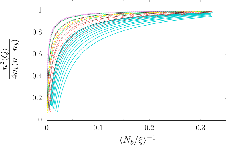
Figure 1: (Color online) Scaled entanglement with respect to the reduced localization length $\langle N_{b}/\xi\rangle^{-1}$ with $N_{b}=\binom{n}{n_{b}}$. The blue thick solid curves correspond to the second band (for $n=11$–$20$), the red thin dashed curves to the third band (for $n=11$–$20$), the green thin dotted curves to the fourth band (for $n=13,15,17$), the black thin solid curves to the fifth band (for $n=10,11,13,15$), the yellow thick dashed curve to the sixth band (for $n=12$), and the violet thick dotted curve to the seventh band (for $n=14$).

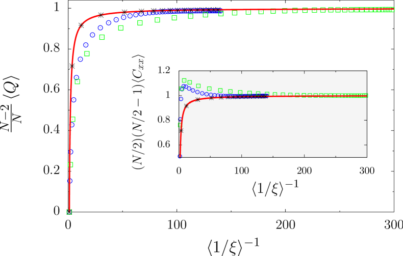
Figure 2: (Color online) Scaled mean MWE $\langle Q\rangle(N-2)/N$ of (9) vs IPR for $\delta=\Delta_{0}$, $n=10$ (blue circles) and $n=11$ (green squares). Average is over $N/16$ central eigenstates and $100-200$ disorder realizations. Red solid line is the theory, and stars are the data for $n=10$ with random shuffling of components. Inset: scaled correlator $(N/2)(N/2-1)\langle C_{xx}\rangle$ with same parameters; red line is the result when $\langle C_{xx}\rangle=\langle C_{xy}\rangle$.

In the case where $\delta\approx\Delta_{0}$, the bands become mixed by the interaction, and delocalization takes place inside the whole Hilbert space. Formula (3) should apply, once modified to take into account the symmetry of the Hamiltonian (9). A straightforward modification of the reasoning leading to Eq. (3) yields $\langle Q\rangle=\frac{N}{N-2}\left(1-\langle\frac{1}{\xi}\rangle\right)$. It turns out that the presence of this particular symmetry allowed the authors of viola to make explicit their formula in a similar case, yielding the same expression as ours.

Figure 2 shows the entanglement of eigenvectors of Hamiltonian (9) compared to this formula. The entanglement goes to one, but departs from the formula at some values of the IPR $\xi$. The inset illustrates that this discrepancy corresponds to a breakdown of the hypothesis $\langle C_{xx}\rangle=\langle C_{xy}\rangle$, because of correlations. These correlations are probably due to the perturbative regime where delocalization takes place on a strongly correlated subset of states. Figure 2 shows that if these correlations are destroyed by random permutations of the components, the results are in perfect agreement with the theory, eventhough the distribution of the component amplitudes is left unchanged. This confirms that (3) can be applied if correlations are weak between the vector components, whatever their distribution.

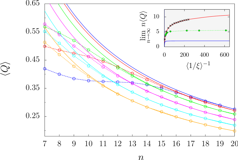
Figure 3: (Color online) Mean MWE vs the number of qubits for 1D Anderson model with disorder from top to bottom $w=0.2$ (blue), $0.5$ (red), $1.0$ (green), $1.5$ (magenta), $2.0$ (cyan), and $2.5$ (orange). Average is over 10 central eigenstates for 1000 disorder realizations. Solid lines are the $C/n$ fits of the tails. Inset: Value of $C=\lim_{n\to\infty}n\langle Q\rangle$ as a function of IPR $\xi$ (green dots) for the values of $w$ above and $w=0.4$, together with analytical result from Eq. (7) (red line, top) and from Eq. (10) (blue line, bottom) both for $M=2\xi$ . Stars are the $C$ values resulting from a $C/n$ fit of the numerical data for CUE vectors of size $N$ with exponential envelope $\exp(-x/l)$.

In the case of localization on adjacent basis vectors, formula (7) can be compared to wavefunctions of electrons in the regime of Anderson localization. Indeed, one dimensional disordered Anderson model is known to display localized eigenstates for any strength of disorder. This type of localization is a one-body phenomenon, but it has been shown that it can be efficiently simulated on a $n$-qubit quantum computer, $\Psi$ describing the particle in the position representation pomeransky . The localization of the particle takes place on a certain number of adjacent computational basis vectors, and the entanglement of the quantum state is related to the entanglement produced by the quantum algorithm. The wavefunctions of the system are known to have an envelope of the form $\exp(-x/l)$ where $l$ is the localization length. For $N$-dimensional CUE vectors with such an exponential envelope, we checked that $\langle Q\rangle$ is in excellent agreement with (7) with $\xi=l$ and $M=2\xi$ (stars in inset of Fig. 3). To test the formula on actual wavefunctions of the Anderson model, we consider a one dimensional chain of vertices with nearest-neighbor coupling and randomly distributed on-site disorder, described by the Hamiltonian $H_{0}+V$. Here $H_{0}$ is a diagonal operator whose elements $\epsilon_{i}$ are Gaussian random variables with variance $w^{2}$, and $V$ is a tridiagonal matrix with non-zero elements only on the first diagonals, equal to the coupling strength, set to $1$. For this system, $\langle...\rangle$ therefore means averaging over the diagonal random values. Figure 3 displays $\langle Q\rangle$ calculated numerically for eigenvectors of this system, as a function of the number $n$ of qubits for various strengths of the disorder $w$. The expected decrease as $C/n$ is perfectly reproduced for large enough values of $n$. The inset shows the value of the constant $C$ compared to the theory (7), as a function of $\xi$. The deviation from (7), in particular the saturation for large $\xi$, can be understood by looking at the structure of eigenvectors in Anderson model: when there is no disorder ($w=0$) the eigenvalues are $E_{k}=2\cos 2\pi\nu_{k}$ and eigenvectors are plane waves with frequency $\nu_{k}$. For weak disorder eigenvectors are exponentially localized with localization length $\xi$ but still oscillate at frequencies distributed as a Lorentzian of width $1/\xi$ around $\nu_{k}$. We chose eigenvectors with energy $E_{k}\approx 0$ ($\nu_{k}\approx 1/4$), yielding rapid oscillations of period 4 which strongly decrease entanglement. It is easy to adapt the analysis leading to Eq. (7) for $\Psi$ chosen as e. g. a vector with $\Psi_{j}=\cos\pi j/2$, $c+1\leq j\leq c+M$, and zero elsewhere. For instance for $M=2^{r_{0}}$, $r_{0}<n$, we get (averaging over $c$)

$$\langle Q\rangle=\Big{(}\frac{26}{9}-\frac{4}{M}-\frac{8(3r_{0}+1)}{9M^{2}}-\frac{4(M^{2}-4)}{3M2^{n}}\Big{)}\frac{1}{n}.$$ (10)

Asymptotically $n\langle Q\rangle$ converges to a constant independent of $\xi=M/2$. The inset of Fig. 3 shows that this theory captures the behavior of the numerical $\langle Q\rangle$, although the saturation constant is different.

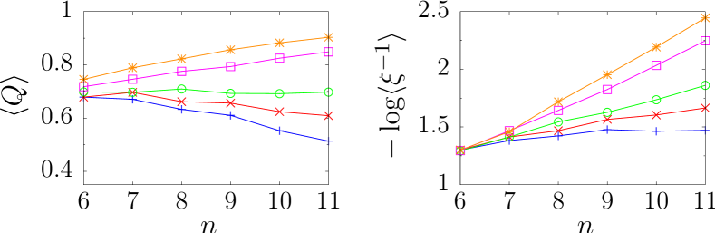
Figure 4: (Color online) Mean MWE (left) and IPR (right) vs number of qubits for quantum smallworld networks with $w=1$ and $p=0.001$ (blue $+$), $0.005$ (red $\times$), $0.01$ (green $\circ$), $0.03$ (magenta $\square$), $0.06$ (orange $\star$). Logarithm is decimal.

Let us now add to this system $pN$ links between randomly chosen vertices. This additional long-range interaction between few vertices turns the system into a quantum smallworld network. Such systems can be efficiently simulated on a quantum computer, and display a localization-delocalization transition for fixed $w$ when $p$ is increased smallworld . Figure 4 shows that this transition can be probed through the entanglement of the system. Indeed, for small $p$ all eigenstates are exponentially localized; $\langle Q\rangle$ is given by (7) and decreases asymptotically as $1/n$; when $p$ is increased the delocalization transition takes place and $\langle Q\rangle$ is now given by Eq. (3): for large $n$, it saturates at $1-\langle 1/\xi\rangle$.

In conclusion, we have shown that in localized random states the mean MWE can be directly related to the IPR $\xi$. Entanglement properties are very different if the localization is on adjacent basis vectors or not. Comparison with physical systems show that global entanglement properties are reproduced, although some discrepancies show that they are much more sensitive than e.g. level statistics to the details of the system.

We thank K. Frahm for helpful discussions, CalMiP and IDRIS for access to their supercomputers, and the French ANR (project INFOSYSQQ) and the IST-FET program of the EC (project EUROSQIP) for funding.

References

- (1) A. Harrow, P. Hayden and D. Leung, Phys. Rev. Lett. 92, 187901 (2004); P. Hayden, D. Leung, P. Shor and A. Winter, Commun. Math. Phys. 250, 371 (2004); C. H. Bennett, P. Hayden, D. Leung, P. Shor and A. Winter, IEEE Trans. Inf. Theory 51, 56 (2005).
- (2) J. Emerson, Y. S. Weinstein, M. Saraceno, S. Lloyd and D. S. Cory, Science 302, 2098 (2003); Y. S. Weinstein and C. S. Hellberg, Phys. Rev. Lett. 95, 030501 (2005).
- (3) H.-J. Sommers and K. Zyczkowski, J. Phys. A 37, 8457 (2004); O. Giraud, J. Phys. A 40, 2793 (2007); M. Znidaric, J. Phys. A 40, F105 (2007).
- (4) R. Jozsa and N. Linden, Proc. R. Soc. A 459, 2011 (2003); G. Vidal, Phys. Rev. Lett. 91, 147902 (2003).
- (5) S. Bettelli and D. L. Shepelyansky, Phys. Rev. A 67, 054303 (2003).
- (6) S. Montangero, Phys. Rev. A 70, 032311 (2004).
- (7) H. Li, X. Wang and B. Hu, J. Phys. A 37, 10665 (2004); H. Li and X. Wang, Modern Physics Letters B 19, 517 (2005).
- (8) L. Viola and W. G. Brown, J. Phys. A 40, 8109 (2007).
- (9) A. D. Meyer and N. R. Wallach, J. Math. Phys. 43, 4273 (2002). G. K. Brennen, Quant. Inf. Comp. 3 619 (2003).
- (10) P. Zanardi, C. Zalka, and L. Faoro, Phys. Rev. A 62, 030301(R) (2000); A.J. Scott and C.M. Caves, J. Phys. A 36, 9553 (2003); A. J. Scott, Phys. Rev. A 69, 052330 (2004). O. Giraud and B. Georgeot, Phys. Rev. A 72, 042312 (2005); S. Montangero and L. Viola, Phys. Rev. A 73, 040302(R) (2006).
- (11) E. Lubkin, J. Math. Phys. (N.Y.) 19, 1028 (1978).
- (12) B. Georgeot and D. L. Shepelyansky, Phys. Rev. E 62, 3504 (2000); Phys. Rev. E 62, 6366 (2000).
- (13) C. Mejia-Monasterio, G. Benenti, G. G. Carlo and G. Casati, Phys. Rev. A 71, 062324 (2005).
- (14) A. A. Pomeransky and D. L. Shepelyansky, Phys. Rev. A 69, 014302 (2004).
- (15) O. Giraud, B. Georgeot and D. L. Shepelyansky, Phys. Rev. E 72, 036203 (2005).