The Orientation of the Reconnection X-line

Abstract

We propose a criterion for identifying the orientation of the X-line when two regions of plasma with arbitrary densities, temperatures, and magnetic fields undergo reconnection. The X-line points in the direction that maximizes the (suitably-defined) Alfvén speed characterizing the reconnection outflow. For many situations a good approximation is that the X-line bisects the angle formed by the magnetic fields.

SWISDAK AND DRAKE X-line Orientation M. Swisdak, IREAP, University of Maryland, College Park, MD 20742-3511, USA, (swisdak@umd.edu)

1 Introduction

Reconnection is the dominant process by which energy is transferred from the magnetic field to the thermal and bulk motions of the particles in collisionless plasmas such as the magnetosphere and the solar corona. Both theoretical models and numerical simulations of reconnection usually consider highly symmetric cases, e.g., the merging of two plasmas that are identical except for their anti-parallel fields, where symmetry considerations dictate the reconnection plane and the orientation of the X-line (the normal to that plane). Realistic configurations are often more complex, as for instance at the magnetopause where a low-density, strong-field plasma (the magnetosphere) merges at an arbitrary angle with a high-density, weak-field plasma (the magnetosheath).

[Sonnerup (1974)] argued that in such complex systems the orientation of the X-line is fixed by requiring that currents in the reconnection plane vanish, and hence, by Ampère’s Law, that the guide field (the magnetic component parallel to the X-line) in the two plasmas be equal. However this choice has the peculiar consequence that there are some magnetic field configurations for which reconnection cannot occur because the reconnecting components of the field have the same sign. A further concern arises from the observation that when a thermal pressure gradient exists at an X-line the guide field must have spatial variations if the system is to be in total pressure balance. Since there is no a priori reason for assuming thermal pressure gradients vanish at X-lines this calls the primary motivation for Sonnerup’s choice into question.

We propose a different criterion: reconnection occurs in the plane in which the outflow speed from the X-line (given by an appropriately-defined Alfvén speed) is maximized. With this choice reconnection can occur between any plasmas in which the magnetic fields are not exactly parallel. Reassuringly, the orientation of the X-line also reduces to the expected result in symmetric cases.

2 Definition of Coordinates

It is particularly important for this problem to define the coordinates carefully. Consider two regions of plasma each with number density $n_{j}$, temperature $T_{j}$, and magnetic field $\mathbf{B}_{j}$, where $j=1,2$. Assume that the two regions are separated by a planar discontinuity through which no magnetic field passes and define a coordinate system in which the $x$ and $z$ axes lie in the discontinuity plane and the $y$ axis is perpendicular to it.

Without any further constraint the X-line could, in principle, point in any direction in the $x-z$ plane. Each different X-line orientation implies a different reconnection plane with different components of the field reconnecting and a different reconnection rate. We want to find the X-line orientation for which reconnection is fastest. To do so it is most convenient not to consider a fixed coordinate system in space but rather to define our coordinates with respect to the direction of the reconnection X-line (the $z$ axis) and the plane of reconnection (the $x-y$ plane) and to rotate the fields about the $y$ axis. This rotation intermixes the guide, $z$, and reconnecting, $x$, components of the fields and changes the reconnection rate. The GSM equivalents of our coordinates at the magnetopause are $(x,y,z)\rightarrow(z,x,y)_{\text{GSM}}$.

Without loss of generality we specify the orientations of the fields by defining $\theta$ to be the angle between the fields on either side of the discontinuity (also called the shear angle) and $\alpha$ as the angle $\mathbf{B}_{1}$ makes with the $z$ axis (see Figure 1). To make the problem well-defined we limit the ranges of the angles: $0\leq\theta\leq\pi$ and $0\leq\alpha\leq\theta$.

The unknown parameter is $\alpha$ and varying $\alpha$ at fixed $\theta$ changes the relative orientations of the fields with respect to the X-line. According to Sonnerup’s argument $\alpha$ is the solution of the equation $B_{1}\cos\alpha=B_{2}\cos(\theta-\alpha)$. We claim that the proper choice is instead the $\alpha$ that maximizes the outflow speed and the rate of reconnection.

As an example, consider a system with $\theta=\pi$, $\mathbf{B}_{1}=-\mathbf{B}_{2}$, $n_{1}=n_{2}$, and $T_{1}=T_{2}$. These parameters describe anti-parallel reconnection and symmetry suggests that $\alpha=\pi/2=\theta/2$. Adding a constant guide field will change $\theta$ but should keep $\alpha=\theta/2$. Sonnerup’s criterion gives the expected results in these cases and ours, as will be seen, does as well. For other parameters, however, the two differ.

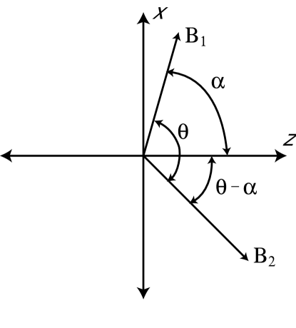
Figure 1: Definition of the coordinate system. The plasmas meet in the plane shown, with one extending out of the page and the other into the page. The shear angle $\theta$ and the directions of the $x$ and $z$ axes are fixed; $\alpha$ is unknown.

3 Determining $\alpha$

The rate at which magnetic field lines reconnect directly varies with the speed at which they flow toward the X-line. Continuity suggests that the speed of this inflow is proportional to the speed of the field lines’ outflow, with a constant of proportionality that depends on the detailed physics of the reconnection (e.g., the aspect ratio of the diffusion region). For our purposes the details of the dependence do not matter; the crucial point is that as the outflow speed increases the reconnection rate does as well.

Since the outflow is driven by the motion of magnetic field lines it must be related to some Alfvén speed; for symmetric anti-parallel reconnection it is the speed calculated from the asymptotic field and density. Defining the appropriate outflow speed in the general case is more complicated. We find that it depends on the fields and densities in both plasmas as well as the angles $\theta$ and $\alpha$. Hence, the inflow speed and reconnection rate depend on these quantities as well.

3.1 Constructing the outflow speed

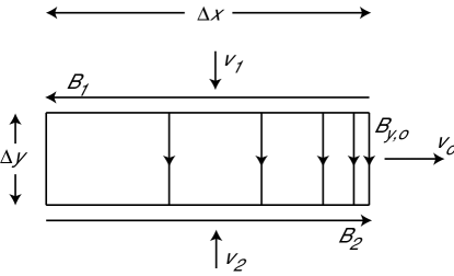
Figure 2: Cartoon of the current layer during asymmetric reconnection. The X-line is at the left of the box and the asymptotic outflow is at the right. All speeds and magnetic field strengths are assumed to be positive.

Consider the situation shown in Figure 2. The left side of the box is the X-line where the plasma velocity and in-plane magnetic field are assumed to vanish. The plasma above the current sheet has mass density $\rho_{1}=m_{1}n_{1}$, where $m_{1}$ is the average mass, and in-plane magnetic field $B_{x,1}$; below the current sheet these values are $\rho_{2}$ and $B_{x,2}$. The plasmas flow into the current sheet with speeds $v_{1}$ and $v_{2}$. Within the current sheet they mix in some proportion, resulting in a plasma of density $\rho_{0}$, and accelerate downstream, dragged by the tension of the reconnected magnetic field. At the right-hand edge of the sheet the plasma reaches its outflow speed $v_{0}$ and the in-plane field has a magnitude $B_{y,0}$. We assume the system is in a steady-state and proceed to calculate $v_{0}$.

Applying conservation of mass to the box gives

$$\rho_{0}v_{o}\Delta y=\rho_{1}v_{1}\Delta x+\rho_{2}v_{2}\Delta x\,.$$ (1)

The out-of-plane electric field $E_{z}$ is, according to Faraday’s Law, spatially constant in a 2-D steady-state system and, asymptotically, must be given by the MHD result $\mathbf{E}=-\mathbf{v}\bm{\times}\mathbf{B}/c$. Equating the values at the inflow and outflow edges of the current layer gives

$$v_{1}B_{x,1}=v_{2}B_{x,2}=v_{0}B_{y,0}\,;$$ (2)

combining equations (1) and (2) yields an expression for $\rho_{0}$

$$\rho_{0}=B_{y,0}\frac{\Delta x}{\Delta y}\left(\frac{\rho_{1}}{B_{x,1}}+\frac{\rho_{2}}{B_{x,2}}\right)\,.$$ (3)

Within the current layer the dominant terms in the $x$ component of the momentum equation are advection and magnetic tension:

$$\rho_{0}v_{x}\frac{\partial v_{x}}{\partial x}=\frac{1}{4\pi}B_{y}\frac{\partial B_{x}}{\partial y}\,.$$ (4)

We assume $B_{x}$ varies piecewise-linearly across the current layer and rewrite this equation as

$$\frac{\partial}{\partial x}\,v_{x}^{2}=\frac{1}{4\pi}\frac{B_{y}}{\rho_{0}}\frac{B_{x,1}+B_{x,2}}{\Delta y}\,.$$ (5)

After integrating with respect to $x$ along the current layer we have

$$v_{o}^{2}=\frac{1}{4\pi}\frac{B_{y,0}}{\rho_{0}}\frac{\Delta x}{\Delta y}(B_{x,1}+B_{x,2})\,,$$ (6)

where $\int B_{y}\,dx=B_{y,0}\Delta x$. Combining equations (3) and (6) gives the outflow speed

$$v_{0}^{2}=\frac{B_{1x}+B_{2x}}{4\pi}\left(\frac{\rho_{1}}{B_{1x}}+\frac{\rho_{2}}{B_{2x}}\right)^{-1}.$$ (7)

Equation (7) exhibits the necessary symmetry between the two sides, reduces to the usual result, $v_{0}^{2}=B_{x}^{2}/4\pi\rho$, when $\rho_{1}=\rho_{2}$ and $B_{1x}=B_{2x}$, and goes to zero, as expected, when either density is large or either field vanishes. This result was independently derived in a slightly different context by [Cassak and Shay (2007)].

In terms of the angles defined in Figure 1 the outflow speed is

$$v_{0}^{2}=\frac{B_{1}\sin\alpha+B_{2}\sin(\theta-\alpha)}{4\pi}\\ \times\left(\frac{\rho_{1}}{B_{1}\sin\alpha}+\frac{\rho_{2}}{B_{2}\sin(\theta-\alpha)}\right)^{-1}\,.$$ (8)

According to our previous argument the condition $\partial v_{0}^{2}/\partial\alpha=0$ defines the orientation of the X-line.

3.2 Maximal Value

Although the operations required to find an expression for $\alpha$ are straightforward, the actual calculations are a bit tedious. Before presenting the result, we make some observations

1. $v_{0}^{2}(\alpha=0)=v_{0}^{2}(\alpha=\theta)=0$. Since $v_{0}^{2}\geq 0$ the implication is that $v_{0}^{2}$ has at least one maximum in the range $0\leq\alpha\leq\theta$. We strongly suspect, but have not been able to prove, that there is only one maximum.

2. $B_{1}$, $B_{2}$, $\rho_{1}$, and $\rho_{2}$ are independent variables but will only enter the result through the two dimensionless ratios $b=B_{2}/B_{1}$ and $r=\rho_{2}/\rho_{1}$. Hence $\alpha$ is a function of only three parameters: $\theta$, $b$, and $r$.

The solution for $\alpha$ is the root of the equation

$$0=r\sin^{2}\alpha[\sin(\theta-2\alpha)-b\sin(2\theta-2\alpha)]\\ +b\sin^{2}(\theta-\alpha)[\sin 2\alpha+b\sin(\theta-2\alpha)]$$ (9)

subject to the constraint $0\leq\alpha\leq\theta$. By defining $\phi=\theta/2-\alpha$, $\phi_{+}=\theta/2+\phi$, and $\phi_{-}=\theta/2-\phi$ equation (9) can be written in the symmetric form

$$0=r\sin^{2}\phi_{-}[\sin 2\phi-b\sin 2\phi_{+}]\\ +b\sin^{2}\phi_{+}[b\sin 2\phi+\sin 2\phi_{-}]\,.$$ (10)

Although equation (9) must, in general, be numerically solved for $\alpha$, exact solutions are possible in some special cases

1. $\theta=\pi$ (anti-parallel reconnection). In this case $\alpha=\theta/2=\pi/2$, independent of the values of $b$ and $r$.

2. $r=1$ ($\rho_{1}=\rho_{2}$). Regardless of $b$ the maximal value occurs for $\alpha=\theta/2$.

3. $b\gg|1-1/r|$ or $b\ll|1/(1-r)|$. Again the result is $\alpha=\theta/2$. The two limits are complementary in the sense that the system is symmetric under the substitutions $b\rightarrow 1/b_{*}$, $r\rightarrow 1/r_{*}$, $\alpha\rightarrow\theta-\alpha_{*}$.

The last example suggests that $\alpha=\theta/2$ is a good approximation to the exact solution of equation (9) whenever the density ratio is not too much different from $1$. Numerical trials bear this out, as can be seen in Figure 3 which shows results for $b=2,r=0.5$.

Figure 3: Plot of $\alpha$ versus the shear angle $\theta$ for the case $b=2$, $r=0.5$. Note that for Sonnerup’s solution there is no reconnection when $\theta\leq 60^{\circ}$.

Interestingly, since the outflow speed does not directly depend on the temperatures or average masses of the plasmas, neither does $\alpha$ (or, equivalently, the X-line orientation). There is an indirect constraint, however, because the system must also be in total pressure balance,

$$n_{1}T_{1}+\frac{B_{1}^{2}}{8\pi}=n_{2}T_{2}+\frac{B_{2}^{2}}{8\pi}\,,$$ (11)

if our assumption of steady-state reconnection is to be valid. If the temperature and the average mass are equal in the reconnecting plasmas then equation (11) relates $b$ and $r$ to the plasma $\beta$

$$\beta_{1} =\frac{b^{2}-1}{1-r} \qquad\beta_{2} =\frac{r}{b^{2}}\frac{b^{2}-1}{1-r}$$ (12)

$$b^{2} =\frac{1+\beta_{1}}{1+\beta_{2}} \qquad r =\frac{1+\beta_{1}^{-1}}{1+\beta_{2}^{-1}}\,.$$ (13)

If desired the condition of equation (9) can be re-written in terms of $\beta_{1}$ and $\beta_{2}$.

4 Discussion

Establishing the system’s orientation is an important part of the interpretation of spacecraft observations. Beginning with the basic magnetic field data the well-known technique of minimum variance analysis determines the direction normal to the current sheet (the $y$ axis in our coordinates). Determining the direction of the X-line, either through Sonnerup’s criterion (see, for example, [Phan et al. (2006)]) or through equation (9), fixes the geometry of the reconnection, provided only that the system has weak variations along the direction of the X-line. This information is particularly important for those measurements that are to be compared to theoretical models and simulations of reconnection, as will be the case for the upcoming Magnetospheric Multiscale Mission.

Our proposed criterion can be checked with numerical simulations. Since our argument does not depend on the detailed physics of the reconnection, only that the reconnection rate varies with the Alfvén speed, even MHD codes that do not correctly describe fast reconnection should suffice. However such simulations must take care not to impose a reconnection plane a priori by, for example, not being fully three-dimensional.

We emphasize that although we have attempted to calculate the direction of the dominant reconnection X-line in a general current layer in this paper, there are several possibly important effects that have been neglected. First, we cannot exclude the possibility that reconnection may proceed simultaneously at different surfaces and that, as a consequence, the current layer might become fully turbulent (Galeev et al., 1986). Second, effects that preferentially suppress reconnection for some X-line orientations are a possible complication that we have ignored. Swisdak et al. (2003) showed that a thermal pressure gradient across the current layer drives diamagnetic drifts that convect the X-line. As the drift speed approaches the Alfvén speed the reconnection can be completely suppressed. Since the magnitude of the drift varies with the angle $\alpha$, the X-line orientation in such systems may be determined by a trade-off between maximizing the outflow Alfvén speed and minimizing the diamagnetic drift. Other effects, e.g., shear flows in the reconnecting plasmas, could have similar consequences.

Finally, equation (9) determines the local orientation of the X-line based on the parameters of the reconnecting plasmas. But what happens at, for instance, the magnetopause where the shear angle can vary with location due to the combined effects of the dipole tilt of the terrestrial field, the direction of the interplanetary magnetic field, and the curvature of the interface? Both the orientation of the X-line and the reconnection rate will then vary with location with unknown effects on the global configuration of the reconnection. One possibility is that local maxima in the reconnection rate will seed vigorously growing X-lines that propagate outwards (Huba and Rudakov, 2002), perhaps occasionally shifting directions to merge with other reconnecting regions. Depending on the external conditions and length of time the system remains in a steady-state it may have either a few or many simultaneously reconnecting X-lines.

References

- Cassak and Shay (2007) Cassak, P. A., and M. A. Shay (2007), Scaling of asymmetric magnetic reconnection in collisional plasmas, Phys. Plasmas, submitted.
- Galeev et al. (1986) Galeev, A. A., M. M. Kuznetsova, and L. M. Zelenyi (1986), Magnetopause stability threshold for patchy reconnection, Space Sci. Rev., 44, 1–41.
- Huba and Rudakov (2002) Huba, J. D., and L. I. Rudakov (2002), Three-dimensional Hall magnetic reconnection, Phys. Plasmas, 9(11), 4435–4438.
- Phan et al. (2006) Phan, T. D., et al. (2006), A magnetic reconnection X-line extending more than 390 Earth radii in the solar wind, Nature, 439, 175–178, 10.1038/nature04393.
- Sonnerup (1974) Sonnerup, B. U. Ö. (1974), Magnetopause reconnection rate, J. Geophys. Res., 79(10), 1546–1549.
- Swisdak et al. (2003) Swisdak, M., B. N. Rogers, J. F. Drake, and M. A. Shay (2003), Diamagnetic suppression of component magnetic reconnection at the magnetopause, J. Geophys. Res., 108(A5), 1218, 10.1029/2002JA009726.