The nature of a broad line radio galaxy: Simultaneous RXTE and Chandra HETG observations of 3C 382

Abstract

We present the results from simultaneous Chandra and RXTE observations of the X-ray bright Broad-Line Radio Galaxy (BLRG) 3C 382. The long (120 ks) exposure with Chandra HETG allows a detailed study of the soft X-ray continuum and of the narrow component of the Fe K$\alpha$ line. The RXTE PCA data are used to put an upper limit on the broad line component and constrain the hard X-ray continuum. A strong soft excess below 1 keV is observed in the time-averaged HETG spectrum, which can be parameterized with a steep power law or a thermal model. The flux variability at low energies indicates that the origin of the soft excess cannot be entirely ascribed to the circumnuclear diffuse emission, detected by Chandra on scales of 20–30″ (22–33 kpc). A narrow ($\sigma<$ 90 eV) Fe K$\alpha$ line (with EW$<$ 100 eV) is observed by the Chandra HEG. Similar values for the line parameters are measured by the RXTE PCA, suggesting that the contribution from a broad line component is negligible. The fact that the exposure is split into two observations taken three days apart allows us to investigate the spectral and temporal evolution of the source on different timescales. Significant flux variability associated with spectral changes is observed on timescales of hours and days. The spectral variability is similar to that observed in radio-quiet AGN ruling out a jet-dominated origin of the X-rays.

1 Introduction

Our understanding of Active Galactic Nuclei (AGN) is based primarily on radio-quiet (RQ) sources, both at high and low luminosities. Multi-wavelength observations of Seyfert galaxies provided us with the widely accepted view that these sources are powered by accretion of gas onto a supermassive central black hole, where the emitted light (optical through X-ray) is produced by an accretion disk and a hot corona overlaying it (e.g., Haardt & Maraschi 1991).

On the other hand, not much is known about the central engines of radio-loud (RL) AGN, due to their relatively low number density (i.e., fewer bright examples). X-ray and multi-wavelength studies of broad line radio galaxies (BLRGs), with $L_{\rm 2-10\;keV}\sim 10^{43}-10^{44}$ erg s^-1, established that these sources exhibit subtle but significant differences compared to Seyfert 1s. While their optical and UV continuum and line emission are similar to those of Seyfert 1 galaxies, BLRGs differ from Seyfert galaxies in their X-ray spectral properties. Specifically, previous ASCA, RXTE  and BeppoSAX observations of BLRGs showed weaker Fe K$\alpha$ lines and weak or absent Compton reflection humps at energies ${\;\mathop{}^{>}_{\sim}\;}10$ keV, a hallmark of Seyfert 1 galaxies (e.g., Woźniak et al. 1998; Sambruna et al. 1999; Eracleous et al. 2000; Zdziarski & Grandi 2001; Hasenkopf, Sambruna, & Eracleous 2002; Grandi et al. 2006). These observations, however, were plagued by limited sensitivity, spectral resolution, and/or the fact that observations in contiguous bands were not simultaneous and were subject to flux and spectral variability.

The weakness of the Fe K$\alpha$ line and of the Compton reflection are very important observational clues, since they represent a major difference between RL and RQ AGN. The origin of this difference, however, is still debated. The simplest interpretation is that the cold reprocessor in RL objects subtends a smaller solid angle to the central X-ray source. This would be the case if the inner accretion disk was vertically extended as in the ion torus/advection dominated flow models (Rees et al. 1982; Narayan et al. 1998). In such a scenario, the RL/RQ dichotomy is caused by different inner accretion disk structures. Alternatively, the weak reprocessing features in RL objects might be explained by dilution effects caused by beamed emission from an unresolved jet. Another possibility is that the putative hot corona has a mildly relativistic motion directed away from the disk reducing the strength of the reflection (Beloborodov 1999; Malzac et al. 2001). Finally, BLRGs might have more highly ionized accretion disks than Seyfert 1 galaxies, as a result of higher accretion rates (e.g., Nayakshin & Kallman 2001; Ballantyne et al. 2002). Detailed studies of ionized accretion disk models (e.g., Matt et al. 1993, 1996; Ross & Fabian 2005) have demonstrated that a progressive increase of the ionization parameter, $\xi=4\pi F_{\rm x}/n$ (where $F_{\rm x}$ is the X-ray flux and $n$ the electron number density), produces several emission lines (e.g., OVII, OVIII, and Fe L lines) in the soft energy band as well as a shift of the energy centroid of the Fe K$\alpha$ line from 6.4 keV to 6.7–6.9 keV. However, when the disk is very strongly ionized with $\xi>5000{~{}\rm erg~{}cm~{}s^{-1}}$ , the resulting X-ray spectrum becomes virtually featureless, because all the electrons have been stripped off the atoms. In the framework of ionized accretion disk models, the weakness of Fe K line can also be explained by lower values of the ionization parameter ($\xi\sim 1000{~{}\rm erg~{}cm~{}s^{-1}}$) provided that strong relativistic blurring effects are included (e.g., Crummy et al. 2006). Interestingly, the latter model is also able to self-consistently account for the presence of a strong soft excess.

Unfortunately, time-averaged spectra alone are unable to break this degeneracy, even using broad-band X-ray data with the highest signal-to-noise (S/N) currently available. This is illustrated by recent XMM-Newton observations of 3C 120 (Ballantyne et al. 2004; Ogle et al. 2005) and 3C 111 (Lewis et al. 2005). In the EPIC spectra the inferred shape of the Fe K$\alpha$ line profile depends sensitively on the adopted shape of the underlying 0.5–10 keV continuum. The continuum can be described equally well by very different models, e.g., a simple power law (yielding broad lines) and a dual absorber (yielding narrow lines).

Here we discuss in detail simultaneous RXTE and Chandra HETG observations of 3C 382, and our attempt to exploit the complementary capabilities of these two satellites. The long (120ks) exposure with Chandra HETG allows a detailed study of the soft X-ray continuum and of the narrow component of the Fe K$\alpha$ line. The RXTE PCA data, on the other hand, are used to constrain the broad line component as well as the hard X-ray continuum. The fact that the exposure is split into two observations taken three days apart allows one to investigate the spectral and temporal evolution of the source on different timescales. Finally, we take advantage of the unprecedented spatial resolution of Chandra to study the physical conditions of the circum-nuclear region.

3C 382 is a nearby ($z=0.058$), well-studied BLRG with strong and variable, broad optical lines (FWHM$\sim 11,800~{}{{\rm km~{}s^{-1}}}$ for H$\alpha$; Eracleous & Halpern 1994). It exhibits a classical Fanaroff-Riley II radio morphology, with a 1.68′–long jet extending NE of the core and two radio lobes, with total extension of 3′ (Black et al. 1992). The inferred inclination angle of the jet of 3C 382 is $i>15$° (Eracleous & Halpern 1998). The nucleus of 3C 382 is a bright X-ray source (F${}_{\rm 2-10~{}keV}\sim 3\times 10^{-11}$ erg cm^-2 s^-1). The 2–10 keV X-ray spectrum is well fitted with a single power law; when the fit to the hard X-ray spectrum is extrapolated to lower energies, a strong soft excess is observed (Prieto 2000; Grandi et al. 2001). ROSAT observations with the High Resolution Imager (HRI) revealed extended X-ray emission around 3C 382 (Prieto 2000). Previous ASCA, BeppoSAX, and RXTE observations showed the presence of a relatively strong Fe K$\alpha$ line, with $F_{\rm line}{\;\mathop{}^{>}_{\sim}\;}10^{-5}~{}{\rm ph~{}cm^{-2}~{}s^{-1}}$ (Woźniak et al. 1998; Sambruna et al. 1999; Eracleous et al. 2000; Grandi et al. 2001), similar to the Seyfert 1 NGC 5548 studied with the HETG (Yaqoob et al. 2001). The line equivalent width in 3C 382 ranges from EW=100 eV to EW=700 eV, depending on the modeling of the underlying continuum. The limited sensitivity and resolution of previous X-ray missions prevented unambiguous modeling of the line and different profiles were derived by different investigators (as discussed in Woźniak et al. 1998; Sambruna et al. 1999; and Zdziarski & Grandi 2001).

The outline of the paper is as follows. In $\S~{}2$ we describe the observations and data reduction. The extended circum-nuclear region is studied in $\S~{}3$. The main characteristics of the temporal analysis are described in $\S~{}4$. In $\S~{}5$ we investigate the spectral properties of the continuum and Fe K$\alpha$ line in 3C 382. In $\S~{}6$ we summarize the main results from the temporal, spectral, and spatial analyses and discuss their implications.

2 Observations and Data Reduction

3C 382 was observed simultaneously with RXTE and Chandra in October 2004. Both observations were split in two parts: RXTE observed 3C 382 between October 27 UT 07:16:41 and 28 UT 09:55:15 (net exposure 32.0 ks), and again between October 30 UT 04:28:16 and 31 UT 06:09:15 (exposure 37.8 ks). Similarly, the Chandra observations were performed on October 27 UT 16:50:39 and 28 UT 08:43:45 (exposure 54.2 ks), and between October 30 UT 07:05:20 and 31 UT 01:37:57 (exposure 63.9 ks).

The RXTE observations were carried out with the Proportional Counter Array (PCA; Jahoda et al. 1996), and the High-Energy X-Ray Timing Experiment (HEXTE; Rotschild et al. 1998) on RXTE. Here we will consider only PCA data, because the signal-to-noise of the HEXTE data is too low for a meaningful analysis. The PCA data were screened according to the following acceptance criteria: the satellite was out of the South Atlantic Anomaly (SAA) for at least 30 minutes, the Earth elevation angle was $\geq 10^{\circ}$, the offset from the nominal optical position was $\leq 0^{\circ}\!\!.02$, and the parameter ELECTRON-2 was $\leq 0.1$. The last criterion excludes data with high particle background rates in the Proportional Counter Units (PCUs). The PCA background spectra and light curves were determined using the ${\rm L}7-240$ model developed at the RXTE Guest Observer Facility (GOF) This model is implemented by the program pcabackest v.2.1b and is applicable to “faint” sources, i.e., those with count rates $<40{\rm s^{-1}~{}PCU^{-1}}$. All the above tasks were carried out with the help of the REX script provided by the RXTE GOF, which calls the relevant programs from the FTOOLS v.5.3.1 software package and also produces response matrices and effective area curves for the specific time of the observation. Data were initially extracted with 16 s time resolution and then re-binned to different bin widths for different applications. The current temporal analysis is restricted to PCA, STANDARD-2 mode, 2–20 keV, Layer 1 data, because that is where the PCA is best calibrated and most sensitive. PCUs 0 and 2 were turned on throughout the monitoring campaign. However, since the propane layer on PCU0 was damaged in May 2000, causing a systematic increase of the background, we conservatively use only PCU2 for our analysis. All quoted count rates are therefore for one PCU. We used PCA response matrices and effective area curves created specifically for the individual observations by the program pcarsp, taking into account the evolution of the detector properties. All the spectra were re-binned so that each bin contained enough counts for the $\chi^{2}$ statistic to be valid. Fits were performed in the energy range 3–15 keV, where the signal-to-noise ratio is the highest.

The Chandra observation was performed with the High Energy Transmission Grating Spectrometer (HETGS; Markert et al. 1994) in the focal plane of the High Resolution Mirror Assembly. HETGS consists of two grating assemblies: a High Energy Grating (HEG; 0.7–10 keV) and a Medium Energy Grating (MEG; 0.4–10 keV). The HEG offers the best spectral resolution in the $\sim 6-7$ keV Fe-K band currently available ($\sim 39$ eV, or $1860\rm\ km\ s^{-1}$ FWHM at 6.4 keV). The MEG spectral resolution is only half that of the HEG. The HEG also has higher effective area in the Fe-K band. The HEG and MEG energy bands are $\sim 0.9-10$ keV and $\sim 0.4-8$ keV respectively, but the effective area falls off rapidly with energy near both ends of each bandpass. The Chandra data were reprocessed with version CIAO version 3.2.1. and CALDB version 3.0.1. Spectral redistribution matrices (rmf files) were made with the CIAO tool mkgrmf for each arm ($-1$ and $+1$) for the first order data of each of the gratings, HEG and MEG. Telescope effective area files were made with the CIAO script fullgarf which drives the CIAO tool mkgarf. Again, separate files were made for each arm for each grating for the first order. The effective areas were corrected for the time-dependent low-energy degradation of the ACIS CCDs using the option available in the mkgarf tool in the stated version of the CIAO and CALDB distribution. Events were extracted from the $-1$ and $+1$ arms of the HEG and MEG using strips of width $\pm 3.6$ arcseconds in the cross-dispersion direction. Light curves and spectra were made from these events and the spectral fitting described later was performed on first-order spectra that were either combined from the $-1$ and $+1$ orders (using response files combined with appropriate weighting), or on first-order spectra from the individual $-1$ or $+1$ orders using the appropriate response files. The background was not subtracted as it is negligible in the energy ranges of interest. Examination of the image of the entire detector and cross-dispersion profiles confirmed that there were no nearby sources contaminating the data.

The spectral analysis was performed using the XSPEC v.12.3 software package (Arnaud 1996). The uncertainties on spectral parameters correspond to the 90% confidence level for one parameter of interest ($\Delta\chi^{2}$ or $\Delta C=2.71$), and the corresponding luminosities are calculated assuming $H_{0}=71{\rm~{}km~{}s^{-1}~{}Mpc^{-1}}$, $\Omega_{\Lambda}=0.73$ and $\Omega_{\rm M}=0.27$ (Bennet et al. 2003). With this choice the luminosity distance of 3C 382 is 256 Mpc.

3 Extended circum-nuclear region

Previous observations of 3C 382 with the ROSAT HRI (with spatial resolution $\sim 4$″) revealed the presence of extended X-ray (0.2–2.4 keV) emission around the source, suggesting that the soft excess of 3C 382 is thermal emission of the extended host gas (Prieto 2000). This interpretation was questioned by Grandi et al. (2001) on the basis of BeppoSAX spectral results that are characterized by higher S/N but encompass a region of 4′. Here we use the high spatial resolution of Chandra ACIS-S coupled with its good sensitivity to clarify this issue.

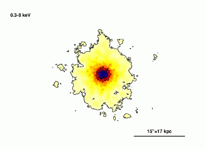
Figure 1: ACIS-S/HETGS zeroth order image of 3C 382 in the 0.3–8 keV band. The image was smoothed using the sub-package fadapt of FTOOLS with a circular top hat filter of adaptive size, adjusted so as to include a minimum number of 10 counts under the filter; each final pixel is 0$\farcs$1.

Inspection of the 0.3–8 keV image of 3C 382 (see Fig. 1) confirms the presence of faint diffuse emission around the core, without any indication for a jet-like structure. To investigate the properties of the extended region in a quantitative way, we extracted a surface-brightness profile from a series of concentric annuli centered on the position of the central source. Then, the radial profile was fitted with a model including the instrument Point Spread Function (PSF). The PSF was created using the Chandra Ray Tracer (ChaRT) simulator which takes into account the spectrum of the source and its location on the CCD (in our case, we used the best-fitting X-ray continuum summarized in Table 1 and discussed in §5).

The observed radial profile of 3C 382 in the total energy band 0.3–8 keV is shown in Figure 2. The PSF model was normalized to the second point of the radial profile ($\sim 1$$\farcs$5) because the inner region is affected by photon pile-up and thus the radial profile is distorted. Comparing the observed data with the instrumental PSF (dashed line) plus background (dotted line), excess X-ray flux over the model is apparent between 6 and 20–30″ (see Fig. 2 bottom panel), indicating the presence of diffuse emission around the core. To model this component, we used a $\beta$ model, described by the following formula (e.g., Cavaliere & Fusco-Femiano 1976):

$$S(r)=S_{0}\left(1+{r^{2}\over r_{c}^{2}}\right)^{-3\beta+1/2},$$ (1)

where $r_{c}$ is the core radius. The radial profile was then fitted with a model including the PSF, the background and a $\beta$-model. The $\beta$-model is required at P${}_{F}\gg$ 99.9% confidence according to an $F$-test. The fitted parameters are: $S_{0}=(7.3\pm 3.4)\times 10^{-5}{\rm~{}ct~{}s^{-1}~{}arcsec^{-2}}$, $\beta=0.48\pm 0.05$, $r_{c}=(6.5\pm 3.1)$″, or $\sim$7.2 kpc. The best-fit $\beta$ model is plotted in Figure 2 (dot-dashed line). The middle panel show the data-to-model ratio when a $\beta$-model is included in the the fit.

We extracted the 0.5–8 keV spectrum of the diffuse emission from an annular region of inner and outer radii of 3″ and 20″, respectively. This spectrum was fitted with a model comprising either an optically thick or optically thin thermal component (bbody or bremss in xspec) and a power-law component, with Galactic absorption affecting both components. The resulting photon index of the power-law component is quite low: $\Gamma=0.9\pm 0.1$; the temperature is $kT=0.17\pm 0.02$ for the blackbody model, or $kT=0.45\pm 0.10$ if a Bremsstrahlung model is used. If the soft component is fitted with a collisionally-ionized plasma model (apec in xspec), at least two components at different temperatures are required ($kT_{1}=0.26_{-0.08}^{+0.15}$ keV and $kT_{2}=1.2_{-0.3}^{+1.6}$ keV) and the abundances are implausibly low ($Z\ll 0.1\;Z_{\odot}$). Assuming a thermal Bremsstrahlung model, the observed flux of the thermal component is $F_{\rm 0.3-2~{}keV}=4.2\times 10^{-13}$ erg cm^-2 s^-1 and the corresponding intrinsic luminosity $L_{\rm 0.3-2~{}keV}=6.6\times 10^{42}$ erg s^-1. Slightly lower values are obtained using a black body model for this spectral component. The power-law component accounts for $\sim 30$% of the total X-ray emission in the 0.3–2 keV range.

The derived luminosity, associated with the extended component in 3C 382, is slightly higher than that found in normal elliptical galaxies (Canizares, Fabbiano, & Trinchieri 1987), and broadly consistent with the values found in low-power radio galaxies (Worrall & Birkinshaw 1994). The luminosity associated with the power-law component, $L_{\rm 0.3-8~{}keV}\sim 1.4\times 10^{43}$erg s^-1, is quite large and cannot be ascribed to the integrated luminosities of X-ray binaries in the host galaxies (see, e.g., Flohic et al. 2006 and references therein). Instead, the power-law component might be related to the emission from the large-scale jet that is unresolved in the X-ray image or to a non-thermal halo already observed in in nearby group of galaxies (Fukazawa et al. 2001) and in the X-ray bright radio galaxy NGC 6251 (Sambruna et al. 2004).

4 Temporal Analysis

The fact that RXTE and Chandra observations were split into two parts taken 3 days apart allows us investigation of the temporal and spectral variability on timescales ranging from few ks to few days. Between the first and the second exposure, the RXTE PCA count rate decreased from $5.70\pm 0.02~{}{\rm s}^{-1}$ to $5.13\pm 0.02~{}{\rm s}^{-1}$ in the 2–15 keV energy band. Similarly, the Chandra HEG (1–8 keV) count rate decreased from $0.205\pm 0.002~{}{\rm s}^{-1}$ to $0.174\pm 0.001~{}{\rm s}^{-1}$, and the MEG count rate (0.4–5 keV) from $0.468\pm 0.002~{}{\rm s}^{-1}$ to $0.393\pm 0.002~{}{\rm s}^{-1}$. In order to check whether the variability shown by MEG data is associated with the softest part of the spectrum, we have restricted the energy band to 0.4–1 keV, which has no overlapping with the HEG range. The results ($0.0588\pm 0.0009~{}{\rm s}^{-1}$ during the first observation and $0.0487\pm 0.0007~{}{\rm s}^{-1}$ during the second one) indicate that the amplitude of variability is even more pronounced in the softer energy band.

This corresponds to a decrease in the average count rate of 3C 382 by factors of 10%, 15%, and 17% in the hard (2–15 keV), medium (1–8 keV), and soft band (0.4–1 keV), respectively, over a time interval of 2 days.

4.1 The X-ray light curve

Figure 3 shows the RXTE PCA light curve in the 2–15 keV energy band (top panel) and the Chandra HETGS light curve in the 0.8–7 keV range (bottom panel). Time bins are 5760 s ($\sim$ 1 RXTE orbit) for RXTE and 2560 s for the HETGS light curve.

A visual inspection of Fig. 3 indicates that the RXTE and Chandra light curves are broadly consistent with each other on long timescales, which are characterized by an overall decrease of the count rate. This variability is formally confirmed by a $\chi^{2}$ test: $\chi^{2}=683.9$ for 26 degrees of freedom (hereafter dof) in the case of RXTE and $\chi^{2}=1019.3$ (45 dof) for the Chandra data. Also on shorter timescales (i.e., within individual exposures), the RXTE light curves show significant variability: during the first exposure, the RXTE light curve shows a steady increase of the count rate by a factor $\sim$10% ($\chi^{2}=44.4$, 12 dof), whereas in the second exposure the RXTE count rate steadily decreases by $\sim$10% ($\chi^{2}=33.9$, 13 dof). The time elapsed during the first Chandra exposure is too short to detect any significant variability. However, the second Chandra observation does show significant short-term variability: the probability that the count rate is constant according to a $\chi^{2}$ test is $P_{\chi^{2}}\sim 2\%$ using time bins of 2560 s ($P_{\chi^{2}}<1\%$ for $t_{\rm bin}=5760$ s).

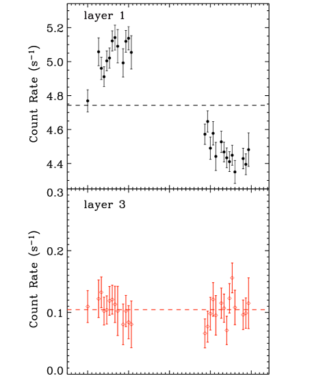
Figure 4: Top panel: RXTE PCA light curve in the 2–10 keV energy band, using PCU2 layer 1. Bottom panel: PCU2 layer 3 light curve. Time bins are 5760 s. The dashed lines are the average count rate level. The signal from the source is expected to be very weak in the layer 3 light curve, thus its variations reflect fluctuations in the background count rate, Note the difference in scale of the y-axes in the two plots. The time is measured relative to 2004 October 27 UT 07:16:41.

Short-term variability may play a significant role in discriminating between competing spectral models for 3C 382 (see discussion below). However, the observed variability amplitude is not very large, thus it is important to verify carefully whether the flux variations are indeed genuine. In particular, it is necessary to demonstrate that the variability observed in 3C 382 cannot be ascribed to uncertainties in the RXTE background. To this end, we have performed the following test: We have compared the background-subtracted light curves obtained using PCU2 layer 1 and PCU2 layer 3. Since the genuine signal in layer 3 is quite small, its light curve can be used as a proxy to check how well the background model works. If the latter light curve is significantly variable with a pattern similar to the one produced using layer 1, then the variability is simply due to un-modeled variations of the background. Conversely, if the PCU2 layer 3 light curve does not show any pronounced variability or if the flux changes are uncorrelated with those observed in the layer 1 light curve, we can safely conclude that the short-term variability detected in 3C 382 is real. The two light curves in the 2–10 keV range (where the background PCA model is better parameterized; see Jahoda et al. 2006 for more details) are shown in Figure 4, revealing that the layer 3 time series is consistent with a constant model (both on long and short timescales) and hence that the variations shown by layer 1 are genuine.

4.2 Spectral variability

In order to investigate whether the flux variability of 3C 382 is associated with spectral variations, we have extracted light curves in two energy-selected bands and defined the hardness ratio as $HR=hard/soft$. For RXTE the soft and hard bands are 2–6 keV and 7–15 keV, whereas 0.4–1 keV and 1–8 keV have been chosen for Chandra. A $\chi^{2}$ test of $HR$ versus time indicates that there is significant spectral variability for RXTE ($\chi^{2}=124.7$, 27 dof) but not for Chandra data ($\chi^{2}=57.2$, 90 dof).

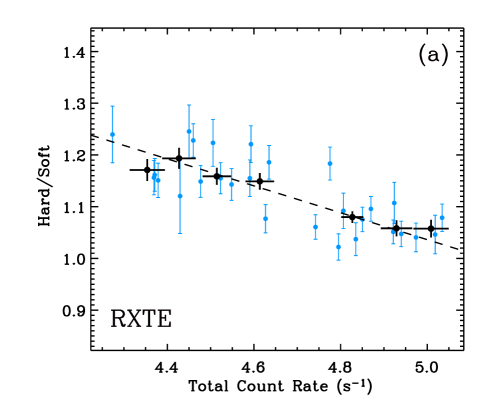
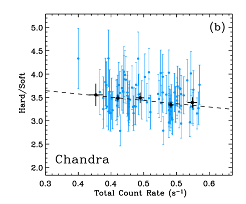
Figure 5: (a): Hardness ratio (7–15 keV/2–6 keV) plotted versus the count rate for RXTE. The gray (blue in color) filled circles correspond to time-bins of 5760 s. The black filled circles are binned points obtained taking the weighted mean of the original points with fixed bins of 0.1 s^-1. The dashed line represent the best-fit model obtained from a least-squares method. (b): HR=(1–8 keV/0.4–1 keV) plotted versus the count rate for Chandra data. Here, the time-bins are 1280 s (gray filled circles) and the black circles are the weighted means with fixed bins of 0.04 s^-1.

A useful method for investigating the nature of spectral variability revealed by the hardness ratio curve is based on the hardness ratio plotted versus the count rate. Figure 5a shows the hard/soft X-ray color plotted versus the count rate for RXTE. The gray (blue in color) filled circles correspond to time-bins of 5760 s. The black filled circles are binned points obtained taking the weighted mean of the original points with fixed bins of 0.1 s^-1. A visual inspection of Figure 5a indicates the presence of a negative trend with the source hardening when the count rate decreases. The dashed line represents the best-fit model to the binned data point, obtained from a least-squares method: $HR=(2.3\pm 0.2)-(0.26\pm 0.03)\;r$ (where $r$ is the count rate). A similar analysis carried out on Chandra data (Fig. 5b), suggests the presence of a similar trend at softer energies, $HR=(4.1\pm 0.5)-(1.40\pm 0.96)\;r$, although at a lower significance level.

The apparent difference between the RXTE and Chandra results can be mostly ascribed to the larger statistical errors associated with the Chandra data, a problem which is exacerbated when dealing with the hardness ratio. The different energy bands probed by the two satellites may also play a role. Indeed, the constant radiation produced by the extended circum-nuclear component peaks around 0.4–1 keV, the soft band probed by Chandra. However, the fact that the largest drop in count rate between observation A and B is measured in the soft band (17% in the 0.4–1 keV range, compared with 15% in 1–8 keV, and 10% in 2–15 keV) seems to argue against this hypothesis.

The observed spectral trend –the softening of the spectrum that accompanies a flux increase– is generally observed in Seyfert-like objects (e.g., Papadakis et al. 2002; Markowitz et al. 2003, and references therein) and can be explained by two alternative models: 1) a two-component model, with two power laws of fixed photon indices and variable normalization for the softer component (e.g., Shih et al. 2002), or 2) a single power law with variable photon index (the “pivoting model”; Zdziarski et al. 2003). Unfortunately, the shortness of the observation and the limited variation of the source’s count rate hampers a more detailed analysis and the possibility of discriminating between the two competing models. Nevertheless, given the similarity between the spectral trend shown by 3C 382 and the one observed in 3C 120 (a BLRG whose behavior has been interpreted in the framework of the pivoting model; Zdziarski & Grandi 2001), it may be instructive to compute the pivot energy, $E_{\rm p}$, for 3C 382. Following Zdziarski et al. (2003), we obtain $E_{\rm p}\simeq 32$ keV.

Another simple way to quantify the variability properties of 3C 382, without considering the time ordering of the values in the light curves, is based on the fractional variability parameter $F_{\rm var}$ (e.g. Rodriguez-Pascual et al. 1997; Vaughan et al. 2003). This is a common measure of the intrinsic variability amplitude relative to the mean count rate, corrected for the effect of random errors, i.e.,

$$F_{\rm var}={(\sigma^{2}-\Delta^{2})^{1/2}\over\langle r\rangle}$$ (2)

where $\sigma^{2}$ is the variance, $\langle r\rangle$ the unweighted mean count rate, and $\Delta^{2}$ the mean square value of the uncertainties associated with each individual count rate. We computed $F_{\rm var}$ on selected energy bands that were chosen to have similar (and sufficiently high) mean count rates in each band. (in the end the count rates range between $\sim$0.35 and $\sim$0.70 s^-1). The plot of $F_{\rm var}$ versus the energy, obtained from RXTE PCA data, is shown in Figure 6. It indicates that the amplitude of variability decreases with increasing energy band, with a minimum around 5.5–6 keV (in the observer frame, where the Fe K$\alpha$ line is located) and then shows a small bump around 8-9 keV. Using Chandra MEG data, we have checked the fractional variability below 1 keV; the value obtained $F_{\rm var,soft}=(6.9\pm 1.6)\times 10^{-2}$ is in broad agreement with RXTE results in the softer energy bands.

Since $F_{\rm var}$ is the square root of the excess variance $\sigma^{2}_{\rm XS}$, introduced by Nandra et al. (1997) and computed for several Seyfert-like objects, we can compare the location of 3C 382 in the $\sigma^{2}_{\rm XS}-L_{\rm 2-10~{}keV}$ plane. With $\sigma^{2}_{\rm XS}\sim 3\times 10^{-3}$ and $L_{\rm 2-10~{}keV}\sim 4.5\times 10^{44}$ erg s^-1, 3C 382 would be located in the lower right corner of Figure 4 of Nandra et al. (1997), following the same anti-correlation trend observed in Seyfert galaxies.

The model-independent information provided by $F_{\rm var}$ spectra has been frequently used to complement the time-averaged spectral analysis. For example, Markowitz et al. (2003) carried out a systematic analysis of the spectral variability properties of Seyfert 1 galaxies observed with RXTE. Their sample includes objects with both broad (e.g., MCG–6–30–15) and narrow (e.g., NGC 4151 and NGC 5548) Fe K$\alpha$ line profiles. Despite the clear difference of the Fe K profiles in the energy spectra, all objects show similar trends in the $F_{\rm var}-E$ plane: $F_{\rm var}$ generally decreases with $E$ reaching a minimum around 6.4 keV and showing a small bump around 8–10 keV. This trend is fully consistent with the one shown by 3C 382 (see Fig. 6) and argues in favor of an accretion-related origin for the bulk of the X-rays. This conclusion is supported by the results from a similar analysis carried out on RXTE observations of the blazar Mrk 501. Indeed, this jet-dominated source shows the opposite trend with $F_{\rm var}$ monotonically increasing with $E$ (Gliozzi et al. 2006).

Although $F_{\rm var}-E$ plots provide us with a useful tool for distinguishing between accretion-related and jet-related X-ray emission for AGN, they do not help us distinguish between competing theoretical models proposed to explain the X-ray energy spectra for AGN, such as reflection-dominated and absorption models (e.g., Gierlinski & Done 2004, 2006). It must be remarked though that using higher-quality XMM-Newton data for MCG–6–30–15, Ponti et al. (2004) were able to demonstrate that the relativistically broadened Fe K$\alpha$ line is revealed in the $F_{\rm var}-E$ plot by a very prominent peak in the $\sim$4.5–6 keV energy band, whereas the narrow line component, presumably produced far away from the inner disk, appears as a narrow dip around 6.4 keV.

In summary, 3C 382 shows significant flux variability in all the energy bands probed on timescales of days and hours. This temporal variability is associated with spectral variability, with the source hardening when the count rate decreases. All the variability properties are consistent with the behavior observed in Seyfert-like objects.

5 Spectral analysis

Previous X-ray studies have shown the spectrum of 3C 382 to be fairly complex and provided remarkably different interpretations of its physical origin. Here, we first investigate the shape of the continuum, combining data from Chandra MEG and HEG, but fitting separately the RXTE PCA data, since the much higher count rate of the latter would dominate and hence bias the fits. Then we focus on the Fe K$\alpha$ line, exploiting the high spectral resolution of the Chandra HETGS and the large collecting area of the RXTE PCA.

5.1 RXTE PCA Continuum

In the previous section, we found evidence that 3C 382 shows spectral variability between the two exposures. To confirm this finding, we fitted separately the 3–15 keV PCA spectra from the two observations with a simple power-law model, modified by Galactic interstellar absorption. The results, $\Gamma_{\rm A}$= 1.78$\pm$0.02 during the first observation (hereafter observation A) and $\Gamma_{\rm B}$=1.72$\pm$0.02 during the second one (observation B) support the suggestion that the spectrum hardens as the source’s count rate decreases.

A simple power-law model (with a Gaussian model parameterizing the Fe K$\alpha$ line) is a good representation of the RXTE spectrum during observation A, but not during observation B, when the spectrum is best fitted by a broken power law with $E_{\rm break}\sim$ 8 keV. The results of the spectral fitting of the PCA data are summarized in Table 1. During observation A, the observed hard X-ray flux and the corresponding luminosity are $F_{\rm 2-10keV}=6.1\times 10^{-11}$erg cm^-2 s^-1 and $L_{\rm 2-10keV}=4.7\times 10^{44}{\rm~{}erg~{}s^{-1}}$. A decrease of $\sim$10% in the flux and luminosity values is observed during observation B.

Since the presence of an energy break close to 10 keV accompanied by a spectral hardening at higher energies is a classic signature of Compton reflection, we have substituted the power law with a pexrav model (which describes the reflection from a neutral disk; see Magdziarz & Zdziarski 1995) in xspec, in order to quantify the contribution from the putative reflection component in 3C 382. Due to the short exposure and the limited energy range, all the pexrav parameters, except the photon index $\Gamma$, the reflection fraction $R$, and the normalization, were kept fixed at reasonable values (we adopted the values given by Eracleous et al. 2000). The spectral fitting suggests that the reflection fraction is more pronounced during observation B ($R\sim$ 0.6) than during the first observation ($R\sim$ 0.2). However, the large uncertainties prevent any firm conclusion; for example, the value of $R$ derived during observation A is consistent with zero at the 90% confidence level. Statistically, these fits are as good as of those obtained using power-law or broken power-law models.

We have also tried to substitute pexrav with the pexriv model, which describes the reflection from an ionized disk (Magdziarz & Zdziarski 1995). The resulting value of the ionization parameter $\xi$ is consistent with zero, although completely unconstrained during observation A. No statistical improvement is obtained with this model. However, the poor spectral resolution of the PCA coupled with the limited energy range non-background-dominated (3–15 keV) hampers the spectral analysis and makes it impossible to constrain the spectral parameters.

5.2 Chandra HETG Continuum

The RXTE PCA spectra are characterized by a high S/N and low spectral resolution, while the opposite is true for the Chandra HETGS spectra. Therefore, in order to study the continuum in the Chandra spectrum we combine the positive and negative grating orders and bin the spectra heavily. The MEG spectra are binned at 0.08 Å, whereas the HEG data are binned at 0.04 Å. All the spectra are grouped to contain at least 15 counts per bin for the $\chi^{2}$ statistic to be valid. Before combining $+1$ and $-1$ orders, we have checked the spectra from individual arms: Spectra of order $-1$ are consistently steeper that those obtained with order $+1$, however, the differences are well within the statistical and systematic errors.

The 2–8 keV HEG spectra confirm the hardening of the source between the two observations: $\Gamma_{\rm A}$=1.70$\pm$0.05 and $\Gamma_{\rm B}$=1.63$\pm$0.05. As already noticed in past studies based on RXTE and Chandra simultaneous observations (e.g., Yaqoob et al. 2003), the HEG photon indices appear to be flatter by ${\;\mathop{}^{<}_{\sim}\;}0.1$ compared to those obtained with the PCA; in any case, the spectral results are consistent within the systematic errors.

If the best-fit power-law model is extrapolated to softer energies combining MEG and HEG data, a strong soft excess below 1 keV is clearly visible (see Fig. 7). A very similar result is obtained if the same procedure is applied to observation B. This clearly indicates that more complex spectral models are necessary to fit also the soft X-ray spectrum of 3C 382.

We fitted the 0.5–8 keV combined MEG and HEG spectra with several phenomenological models, such as a power law describing the hard energy spectrum combined with an additional component (steep power law or thermal component) parameterizing the soft excess. The results of the spectral fitting, summarized in Table 2, indicate that all models are able to fit the broad-band continuum of 3C 382 fairly well. This is confirmed by Figure 8, where the MEG and HEG data from 0.5–8 keV are shown with the double power-law model superimposed. The observed soft X-ray flux and the corresponding luminosity are very similar for all models. During observation A, using the double power-law model we obtain: $F_{\rm 0.4-2keV}=3.2\times 10^{-11}$erg cm^-2 s^-1 and $L_{\rm 0.4-2keV}=3.6\times 10^{44}{\rm~{}erg~{}s^{-1}}$. The values of the flux and luminosity in the 0.4–2 keV band decrease by a factor $\;\mathop{}^{>}_{\sim}\;$15% during observation B.

Despite the formally acceptable fit (see Table 2), the plot of the soft spectrum with the best-fit model superimposed (Fig. 8) suggests the presence of several line-like features in the 0.7–1 keV range (in the observer’s frame). In order to investigate further this issue, after restricting the fitting range to 0.5–1.5 keV, we have tried to add several Gaussians to the underlying continuum. We find that the fit is improved at the 90% confidence level (i.e., $\chi^{2}$ decreases by more than 6.25 for each Gaussian added) by adding two narrow lines. The energy centroids $E_{1}=0.89\pm 0.01$ keV and $E_{2}=1.04\pm 0.01$ keV (in the source rest frame) are consistent with transition from Ne IX and Ne X, respectively. Detailed photoionization modeling may give more insight into the identification of these lines but there is insufficient statistically significant information in the spectrum to warrant more sophisticated modeling.

Similarly to the procedure applied to the PCA data, we used the pexrav model instead of the power law to account for the presence of reflection. Fixing $R$ at the best-fit values obtained from the PCA data, the resulting spectral fits are as good as those obtained using the phenomenological models reported in Table 2. If $R$ is left free to vary, the spectral fits yield $R=0$ with 90% upper limits of 0.3 and 0.6 for observation A and B, respectively. Using the pexriv model with HETG spectra leaves the ionization parameter totally unconstrained.

As an alternative to the phenomenological models described above, we have also tried to fit the HETG spectra with a more physically-motivated model such as reflion (which describes the reflection from an optically-thick atmosphere of constant density; see Ross & Fabian, 2005) in xspec. However, the low S/N of the data in the soft part of the spectrum combined with the limited energy band hampers the analysis and does not allow to constrain the parameters properly. The resulting fit is poor (the soft excess is still present) and the best fit parameters indicate that the fraction of the reflected radiation is quite small($F_{\rm refl}/F_{\rm tot}\sim 10\%$) and also that the ionization parameter is low ($\xi\sim 350-400~{}{\rm erg~{}cm~{}s^{-1}}$). A significant formal improvement in the fit is obtained by convolving the reflection disk model with kdblur to account for the relativistic blurring close to the black hole (see Crummy et al. 2006 for a detailed description of kdblur). In this case the reduced $\chi^{2}$ is comparable to the one obtained with the phenomenological models, but the number of free parameters is significantly larger. However, the fitting procedure becomes extremely slow and the parameters of kdblur (specifically, $r_{\rm in}$, the disk emissivity index, and the inclination angle) remain totally unconstrained. If this model with parameters fixed at their best-fit values is applied to the PCA spectra, the resulting fits are significantly worse than those obtained with power law or pexrav models.

Finally, if the RXTE data are fitted simultaneously with the HETG spectra, an adequate fit of the data ($\chi^{2}_{\rm red}=1.09/536$ for observation A and $\chi^{2}_{\rm red}=1.08/538$ for observation) is obtained using a power law to parameterize the soft excess and a pexrav model to describe the spectrum at higher energies. The resulting deconvolved $E~{}F_{\rm E}$ spectra are shown in Figure 10.

In summary, 3C 382 shows a strong soft excess below 1 keV, when the hard (2–10 keV) photon index is extrapolated at softer energies. The broad-band spectrum is fitted reasonably well by a power law plus a thermal component (or a steep power law). The limited quality of the data hampers the use of more complex spectral models such as ionized disk reflection models. No intrinsic absorption in addition to the Galactic column density is required.

5.3 Fe K$\alpha$ line

We use the complementary characteristics of the Chandra HEG and the RXTE PCA to study the profile origin of the Fe K$\alpha$ line and investigate its origin. Because of its high spectral resolution, the HEG probes the narrow component of the line profile (likely to originate in matter that is not part of the inner accretion disk). In contrast, the PCA is sensitive to the entire Fe K$\alpha$ profile, which may consist of both the narrow and the broad component (the broad component is thought to be produced in the inner part of the accretion disk).

Since we want to test whether the narrow line is resolved by the HEG (the resolution element is 0.012 Å), we use spectra binned at 0.01 Å. To analyze the HEG spectrum, we restrict our fits to the energy range to 3–8 keV and use a power-law model for the local continuum. To judge the goodness of the fit, we use the $C$-statistic. We fit the PCA spectrum in the 3–15 keV range adopting a broken power-law model for the continuum and using the $\chi^{2}$ statistic as an indicator of the goodness of the fit. The profile of the Fe K$\alpha$ line is described by a Gaussian model in all cases.

The results of this analysis are reported in Table 3. The values of the spectral parameters remain basically unchanged when we use higher resolution spectra binned at 0.005 Å. We fitted spectra from different dispersion arms separately and checked the results for consistency. When we use the HEG spectrum of order $+1$ only, the significance of the Fe K$\alpha$ line detection is much higher, therefore, we report both the results obtained after combining the $+1$ and $-1$ orders and those from order $+1$. Using the combined spectrum from both arms, a weak (EW$\sim 20-50$ eV), unresolved line with energy consistent with Fe K$\alpha$ at 6.40 keV is detected at a high confidence level during observation B, but it is only marginally significant during observation A. As expected, the spectral parameters are better determined during observation B, when the continuum level is lower, although there is a substantial agreement between the line parameters during the two observations. It is worth noting that using spectra from dispersion arm +1, the line significance and strength are substantially increased in both observations, and that during observation B the line appears to be resolved ($\sigma=81_{-25}^{+35}$ eV, corresponding to a FWHM of 8900 km s^-1) at the HEG resolution.

The RXTE PCA spectrum, fitted separately, requires a line at $\sim$ 6.4 keV (in the source rest frame) in both observations. Importantly, when fitted with a Gaussian model, the spectral parameters are fully consistent with those obtained with the HEG (see Table 3). In particular, taking into account the systematic error in the RXTE flux (known to be around 10–20% higher than Chandra; see Jahoda et al. 2006), the line intensities measured by the RXTE PCA are in fairly good agreement with those measured by the HEG (see also Fig. 10). This suggests that the Fe K$\alpha$ line in 3C 382 is dominated by a narrow component and that a broad component is not detected. In order to quantitatively constrain the broad line component, we added to the best-fitting continuum a diskline (which describes the profile of a line emitted from a relativistic accretion disk; the parameters were fixed at the following values $r_{i}=6~{}r_{\rm g}$, $r_{o}=400~{}r_{\rm g}$, $q=2.5$, $i=30\arcdeg$, and $E=6.4$ keV; where $r_{\rm g}\equiv GM_{BH}/c^{2}$). The model also includes a narrow Gaussian line. The addition of a broad line component does not improve the fit at all, but it allows the determination of the 90% upper limits on the line equivalent width, wich are 40 eV during observation A and 90 eV during observation B. Similar upper limits are obtained if we use the laor model, which describes the line emission in the hypothesis that the black hole is nearly maximally rotating.

It is instructive to compare the measured Fe K$\alpha$ equivalent widths with the values expected on the basis of the reflection fraction $R=\Omega/2\pi$ obtained by fitting the contimuum with a pexrav model. According to the calculations from George & Fabian (1991), the relation between these two quantities can be expressed as $EW=160(\Omega/2\pi)$ eV, which yields $EW\sim$ 40 eV and $EW\sim$ 100 eV, for observation A and observation B, respectively. These values, which are in general agreement with the measured values of $EW$ (see Table 3), suggest a common physical origin for the Fe K$\alpha$ line and the Compton reflection component.

6 Summary of Results and Discussion

By taking advantage of the complementary capabilities of the RXTE PCA and the Chandra HETGS we have obtained several results on the BLRG 3C 382, which can be summarized as follows:

• A model-independent timing analysis has revealed the existence of significant flux variability on short (few ks) and medium (days) timescales. This temporal variability is accompanied by spectral variability such that the source spectrum hardens as the count rate decreases. The variability amplitude decreases with increasing energy. A potentially important clue is that the soft band shows significant flux variability, coordinated with the hard band, with a similar amplitude. This suggests a close connection between the two energy bands.

• An analysis of the time-averaged spectrum shows the presence of a strong soft excess below 1 keV, when the hard (2–10 keV) power law is extrapolated to lower energies. The broad band spectrum is adequately fitted by a power law plus a thermal model (or a steep power law) describing the soft excess. The spectra are fitted equally well with a neutral reflection model (pexrav). The reflection fraction is poorly constrained during observation A ($R\sim 0.2$ but consistent with zero at the 90% confidence level) and is of the order of 0.6 during observation B, when the continuum flux is lower.

• A weak, narrow iron line with energy centroid consistent with neutral Fe K$\alpha$ is detected by the PCA and the HEG at high confidence level. There is no indication of a relativistically broadened Fe line. The good agreement between the line parameters obtained with the PCA and those yielded by the HEG suggests that the Fe K$\alpha$ line in 3C 382 is dominated by a “narrow” component, probably not originating in the inner accretion disk. The FWHM of the Fe K$\alpha$ line of $8900\pm 3500$ km s^-1  (as measured by HEG+1 during observation B) is comparable to the FWHM of the optical hydrogen Balmer lines of 11,800 km s^-1, suggesting a possible common origin of these lines. The double-peaked optical lines have been attributed to the outer accretion disk (Eracleous & Halpern 1994, 2003), which is also a plausible site for the production of the Fe K$\alpha$ line.

• A spatial analysis based on the radial surface brightness profile confirms the presence of diffuse emission around 3C 382 on scales of the order of 20–30″ corresponding to $\sim 22$–33 kpc. The soft spectrum of the diffuse emission is well described by a thermal model (black body or Bremsstrahlung) with temperatures significantly higher than those describing the soft excess in the AGN spectrum. This result, combined with the variability observed in the soft band, rules out the hypothesis that the soft excess in the AGN spectrum can be explained entirely by the extended emission.

If we compare our spectral results with the most recent X-ray studies of 3C 382 in the literature, i.e. with BeppoSAX analysis of Grandi et al. (2001) and the RXTE investigation from Eracleous et al. (2000), we find a general agreement on the weakness of the iron line: equivalent widths of 50 and 90 eV were measured by BeppoSAX and RXTE, respectively, which are fully consistent with the results reported in Table 3. Also the weak reflection component measured in the continuum, although poorly constrained, is in broad agreement with the results reported in the literature ($\Omega/2\pi\sim 0.5$ by Eracleous et al. 2000; $\Omega/2\pi\sim 0.3$ by Grandi et al. 2001).

Our analysis of the time-averaged spectrum alone has not led to definitive conclusions about the nature of X-ray source in 3C 382. However, the combination of the information from the temporal, spectral, and spatial analyses, can put tighter constraints on 3C 382 with implications for all BLRGs.

Previous studies of time-averaged spectra have shown that several competing scenarios can explain the weak reprocessing features observed in the X-ray spectra BLRGs equally well. In summary, these peculiar X-ray properties can be explained by: 1) an accretion disk truncated at small radii with a radiatively inefficient accretion flow in the central region (RIAF; Eracleous et al. 2000); 2) a highly ionized accretion disk (Ballantyne et al. 2004); 3) a mildly relativistic outflowing corona (Beloborodov 1999); and 4) dilution from jet emission (e.g., Sguera et al. 2005).

To evaluate the above hypotheses we use the black hole mass in 3C 382, obtained from the B-band luminosity of the host galaxy, $M_{BH}=1.1\times 10^{9}{\rm~{}M_{\odot}}$ (with an uncertainty of approximately 40%; Marchesini et al. 2004). We also estimate the bolometric luminosity to be $L_{\rm bol}=9\times 10^{45}~{}{\rm erg~{}s}^{-1}$. Thus we obtain an Eddington ratio of $L_{\rm bol}/L_{\rm Edd}=0.02$–0.2 (including our best estimate of the uncertainties) and a light crossing time of the inner accretion disk of $\tau_{\ell}\equiv 100\;r_{\rm g}/c=2$–5 days. With the above estimates in mind, our results can constrain the proposed scenarios as follows:

• If the inner accretion disk is a radiatively inefficient accretion flow (RIAF), then its size (i.e., $r_{\rm tr}$, the transition radius from the thin disk to the hot, vertically extended flow) is constrained by the observed variability time scale. The dramatic drop in the observed X-ray flux over a timescale of approximately two days, sets a stringent upper limit to the light-crossing time of the RIAF ($r_{\rm tr}<100r_{\rm g}$). Such a small transition radius is not unprecedented (see, for example the application to NGC 4258 by Gammie, Narayan, & Blandford 1999). There are also short-term fluctuations with an amplitude of about 5% superposed on the secular flux changes during our observations, which may result from inhomogeneities in the flow. The inferred Eddington ratio is uncertain enough that its lower limit ($L/L_{\rm Edd}\approx 0.02$) is compatible with presence of a RIAF. For higher values of $L/L_{\rm Edd}$, an inner radiatively inefficient flow might still be a viable solution in the form of the luminous hot accretion flow proposed by Yuan et al. (2007).

• The scenario in which the X-rays are dominated by reflection from a highly ionized accretion disk cannot be firmly ruled out or confirmed by the present data. The time-averaged spectral analysis reveals no clear evidence for a high ionization state. However, if the ionization is very high or if relativistic blurring effects are very strong, no prominent spectral signatures are expected and in any case the current data would not be able to detect them unambiguously. In principle, useful information about this scenario can also be obtained from the estimated accretion rate and from the measured variability. Specifically, all ionized accretion disk models require very high values of $\dot{m}$ to produce high ionization states. However, the uncertainties on the black hole mass and hence on the Eddington ratio estimated for 3C 382 do not allow one to derive firm conclusions from this argument. Finally, the ionized-reflection-dominated scenario, at least in the framework of the photon bending model (see Miniutti & Fabian 2004 and references therein), predicts that the primary (in our case the 2–10 keV component) and the reflection-dominated components (the soft excess) should not vary in concert, when the source is in a bright state. Therefore, the simultaneous flux drop observed for 3C 382 between observation A and B in all the energy bands, seems to argue against the light bending scenario.

• The scenario involving a mildly relativistic outflowing corona seems to be consistent with our results. Indeed, a moderately outflowing corona ($\beta=c/v=0.3$) can naturally explain the relatively flat photon index observed in 3C 382 (Malzac et al. 2001). However, this can only be considered as circumstantial evidence in favor of outflowing corona models, since X-ray slopes flatter than 1.9 can also be produced in the framework of static corona models by assuming patchy configurations (Haardt et al. 1994).

• The jet-dominated scenario does not seem viable, as shown by previous studies of of the time-averaged X-ray spectra of BLRGs (e.g., Woźniak et al. 1998). Our model-independent variability results along with the relatively large viewing angle of the jet in 3C 382 (obtained from radio properties; Rudnick et al. 1986, Eracleous & Halpern 1998) reinforce this conclusion. First, the fast variability we have observed cannot be ascribed to jet emission because of the large viewing angles (i.e., the emission is not beamed). Second, the spectral variability (the spectral hardening when the flux decreases and the anti-correlation of $F_{\rm var}$ with energy) is typical of radio-quiet AGN and at odds with the spectral variability observed in jet-dominated sources (Gliozzi et al. 2006). Nevertheless, we cannot exclude that an appreciable contribution from the jet component may emerge at higher energies, as suggested by recent Suzaku results for the BLRG 3C 120 (Kataoka et al. 2007).

More stringent tests of the above scenarios (especially the first two) will be afforded by more precise measurements of the black hole mass and the bolometric luminosity (hence the Eddington ratio) of 3C 382. A better mass measurement can be made using the stellar velocity dispersion of bulge of the host galaxy (e.g., Ferrarese & Meritt 2000; Gebhardt et al. 2000; Tremaine et al. 2002), a technique which leads to a small systematic error. For a better measurement of the bolometric luminosity, the spectral energy distribution needs to be sampled more densely, especially in the infra-red and ultra-violet bands. Additionally, future observations with Suzaku covering the entire X-ray range from 0.2 keV to several hundreds of keV will be crucial for breaking the current spectral degeneracy.

Before concluding, we can speculate on the origin of the radio-loud/radio-quiet dichotomy by putting into perspective the results of 3C 382. First, our study suggests that jet production may not necessarily be related to a very low value of the accretion rate $\dot{m}$ (if the Eddington ratio is indeed in the range 0.02–0.2). This is in agreement with findings from other BLRGs (e.g., 3C 120; Ballantyne & Fabian 2005, Ogle et al. 2005), radio-loud quasars (Punsly & Tingay 2005), and Galactic black holes (GBHs). In fact, Galactic black holes display relativistic jets not only in the “low-hard” state but also in the “very-high” spectral state that is characterized by a high accretion rate (e.g., Fender et al. 2004). Second, a maximally rotating black hole is not a sufficient condition for jet production (although it may be necessary). We are led to this conclusion by the fact that there isn’t any radio jet in MCG–6–30–15, the well known Seyfert 1 galaxy that shows the most convincing evidence for a spinning black hole based on its relativistically broadened Fe K$\alpha$ line (this galaxy harbors only a weak, unresolved radio source; see Ulvestad & Wilson 1984). This is also consistent with the fact that highly relativistic jets have been observed in neutron star binaries (e.g., Fomalont et al. 2001; Migliari et al. 2006). Having excluded the low $\dot{m}$ and the presence of a spinning black hole, we can speculate that jet production might be related to another parameter, such as a specific topology of the magnetic field in the inner region of the accretion flow. Following Livio et al. (2003), we can hypothesize that jet production is related to formation of a poloidal magnetic field that is triggered by an increase of the fraction of the energy dissipated in the accretion-disk corona. This change might cause the outflow of the corona that, in turn, can explain the observed X-ray properties in BLRGs.

In conclusion, our study of 3C 382 shows the potential benefits of exploiting the complementary capabilities of RXTE and Chandra  and combining model-independent information from spectral variability with the analysis of time-averaged X-ray spectra and morphologies. Extending this approach to a large sample of BLRGs with higher quality data may help reduce the current spectral degeneracy and shed some light in the radio-loud -quiet dichotomy.

Figure 2: X-ray surface brightness profile of 3C 382. The solid line represents the best-fit model, which comprises the PSF model (dashed line), $\beta$–model (dot-dashed line), and the background level (dotted line). The lower panels show the data-to-model ratios in the cases where a $\beta$-model is included or not in the fit. The inner region ($r<2$$\farcs$5) has been excluded from the fit because the core is highly piled-up.

Figure 3: Top panel: RXTE PCA light curve in the 2–15 keV energy band. Bottom panel: Chandra HETG light curve in the 0.8–7 keV range. The dashed lines represent the respective average count rate. Time bins are 5760 s ($\sim$ 1 RXTE orbit) for RXTE and 2560 s for the HETGS light curve. The time is measured relative to 2004 October 27 UT 07:16:41.

Figure 6: Fractional variability parameter plotted versus the energy for using RXTE PCA data. The error-bars along the x axis simply represent the energy band width. The error-bars along the y axis are computed following Vaughan et al. 2003. The energy is in the observer rest frame.

Figure 7: Data/model ratio to a simple power-law model modified by photoelectric absorption in the Milky Way. The data are from the MEG and HEG during the first observation. A strong soft excess in present below 1 keV.

Figure 8: The MEG and HEG spectra in the 0.5–8 keV energy range, obtained combining orders $+1$ and $-1$ during observation A when the mean count rate was higher (a very similar soft spectrum is obtained during observation B). The bin size are 0.08 Å and 0.04 Å for the MEG and HEG, respectively. The continuous line represents a double power-law model absorbed by Galactic $N_{\rm H}$. The bottom panel shows the data/model ratio.

Figure 9: Deconvolved MEG, HEG, and PCA spectra in the 0.5–15 keV energy range, fitted with a power-law plus a neutral reflection model (pexrav) plus a Gaussian line at $\sim$ 6.4 keV in the source’s rest frame. All models are absorbed by Galactic $N_{\rm H}$. Figures (a) and (b) represent observation A and B, respectively.

Figure 10: Confidence contours in the line intensity–line width plane. The confidence levels correspond to 68%, 90%, and 99%. Panel (a) at the top left refers to observation A (HEG$+1$); panel (b) at the top right refers to observation B (HEG$+1$). The bottom panels on the left (c) and right (d) show the confidence contours derived from the PCA spectra during observations A and B, respectively.

Table 1: PCA Continuum Models

(broken) power law
Observation	norm	$\Gamma$	$E_{\rm break}$	$\Gamma_{2}$	$\chi^{2}$/dof
	$(10^{-5})^{a}$		keV
A	$4.3_{-2.0}^{+1.9}$	$1.78_{-.02}^{+.02}$			12.09/24
B	$8.5_{-1.9}^{+2.8}$	$1.76_{-.03}^{+.11}$	$8.4_{-2.5}^{+1.1}$	$1.53_{-.11}^{+.10}$	23.95/21
neutral reflection (pexrav)
Observation	norm	$\Gamma$	R		$\chi^{2}$/dof
	$(10^{-5})^{a}$		$(\Omega/2\pi)$
A	$4.0_{-2.0}^{+1.9}$	$1.79_{-.05}^{+.05}$	$0.23_{-0.23}^{+0.30}$		10.56/23
B	$6.5_{-1.7}^{+1.7}$	$1.80_{-.05}^{+.05}$	$0.62_{-0.31}^{+0.37}$		27.02/22
ionized reflection (pexriv)
Observation	norm	$\Gamma$	R	$\xi$	$\chi^{2}$/dof
	$(10^{-5})^{a}$		$(\Omega/2\pi)$	$({\rm erg~{}cm~{}s^{-1}})$
A	$3.8_{-2.5}^{+3.6}$	$1.80_{-.05}^{+.05}$	$0.24_{-0.24}^{+0.28}$	$0(<5000)$	10.41/23
B	$6.6_{-2.4}^{+1.8}$	$1.80_{-.05}^{+.06}$	$0.60_{-0.26}^{+0.40}$	$0(<40)$	26.83/21

^a Normalization of the power-law model at 1 keV in units of ${\rm~{}ph~{}cm^{-2}~{}s^{-1}~{}keV^{-1}}$.
A narrow ($\sigma=10$ eV) Gaussian line at 6.4 keV (in the source’s rest frame) is required in all the spectral fits. For observation B, we have also included a narrow line at 4.78 keV (in the observer’s frame) to account for the instrumental effect related to the Xe L edge.

Table 2: MEG+HEG Continuum Models

power law plus power law
Observation	norm1	$\Gamma_{\rm soft}$	norm2	$\Gamma_{\rm hard}$	$\chi^{2}$/dof
	$(10^{-3})^{a}$		$(10^{-2})^{a}$
A	$2.8_{-0.7}^{+1.0}$	$4.5_{-0.5}^{+0.5}$	$1.18_{-0.08}^{+0.06}$	$1.60_{-0.05}^{+0.04}$	566.3/563
B	$2.2_{-0.5}^{+0.6}$	$4.6_{-0.4}^{+0.4}$	$0.98_{-0.05}^{+0.04}$	$1.56_{-0.04}^{+0.03}$	569.8/563
black body plus power law
Observation	norm1	$kT$	norm2	$\Gamma$	$\chi^{2}$/dof
	$(10^{-4})^{b}$	(keV)	$(10^{-2})^{a}$
A	$3.5_{-0.6}^{+0.8}$	$0.10_{-0.01}^{+0.01}$	$1.31_{-0.02}^{+0.02}$	$1.69_{-0.02}^{+0.02}$	577.6/564
B	$2.9_{-0.5}^{+0.7}$	$0.10_{-0.01}^{+0.01}$	$1.07_{-0.02}^{+0.02}$	$1.64_{-0.02}^{+0.02}$	575.4/564
bremsstrahlung plus power law
Observation	norm1	$kT$	norm2	$\Gamma$	$\chi^{2}$/dof
	$(10^{-1})^{c}$	(keV)	$(10^{-2})^{a}$
A	$1.3_{-0.2}^{+0.2}$	$0.19_{-0.02}^{+0.03}$	$1.29_{-0.02}^{+0.02}$	$1.68_{-0.02}^{+0.02}$	579.2/564
B	$1.0_{-0.3}^{+0.5}$	$0.20_{-0.02}^{+0.03}$	$1.06_{-0.02}^{+0.02}$	$1.63_{-0.02}^{+0.02}$	574.4/564

^a Normalization of the power-law model at 1 keV in units of ${\rm~{}ph~{}cm^{-2}~{}s^{-1}~{}keV^{-1}}$. ^b Normalization of the black body model at in units of $L_{39}/D^{2}_{10}$, where $L_{39}$ is the source luminosity in ${\rm 10^{39}~{}erg~{}s^{-1}}$ and $D_{10}$ the distance of the source in units of 10 kpc. ^c Normalization of the Bremsstrahlung model; see the Xspec manual for a detailed description.

Table 3: Fe K$\alpha$ Gaussian Model Parameters (Rest Frame)

Observation	Instrument	$E_{\rm Fe}$	$\sigma_{\rm Fe}$	$I_{\rm Fe}$	EW	$\Delta\chi^{2}$/dof
		(keV)	(eV)	($10^{-5}{\rm~{}ph~{}cm^{-2}~{}s^{-1}}$)	(eV)	($\Delta C$/dof)
A	PCA	$6.42_{-0.30}^{+0.30}$	3 ($<$955)	$4.2_{-2.0}^{+2.0}$	$58_{-28}^{+28}$	-13.0/3
A	HEG+1-1	$6.37_{-0.05}^{+0.03}$	1($<$94)	$1.2_{-1.0}^{+1.4}$	$17_{-15}^{+11}$	-3.7/3
A	HEG+1	$6.62_{-0.14}^{+0.01}$	2($<$30)	$2.9_{-1.3}^{+1.5}$	$47_{-22}^{+24}$	-16.1/3
B	PCA	$6.50_{-0.16}^{+0.10}$	5 ($<$356)	$8.3_{-2.0}^{+16}$	$133_{-30}^{+255}$	-54.0/3
B	HEG+1-1	$6.43_{-0.07}^{+0.05}$	6($<$87)	$3.5_{-1.3}^{+2.8}$	$55_{-20}^{+47}$	-10.4/3
B	HEG+1	$6.39_{-0.04}^{+0.03}$	$81_{-25}^{+35}$	$7.3_{-2.2}^{+3.2}$	$132_{-46}^{+42}$	-35.2/3

References

- Arnaud (1996) Arnaud, K. 1996, in ASP Conf. Ser. 101, Astronomical Data Analysis Software and Systems V, ed. G. Jacoby & J. Barnes (San Francisco: ASP), 17
- Ballantyne et al. (2002) Ballatyne, D.R., Ross, R.R., & Fabian, A.C. 2002, MNRAS, 332, 45
- Ballantyne et al. (2004) Ballatyne, D.R., Fabian, A.C., & Iwasawa, K. 2004, MNRAS, 354, 839
- Ballantyne & Fabian (2005) Ballatyne,D.R. & Fabian, A.C., 2005, ApJ, 622, 97
- Beloborodov (1999) Beloborodov, A.M. 1999, ApJ, 510, L123
- Bennet et al. (2003) Bennet, C.L. et al. 2003, ApJS, 148, 1
- Black et al. (1992) Black, A.R.S., Baum, S.A., Leahy, J.P. et al. 1992, MNRAS, 256, 186
- Canizares et al. (1987) Canizares, C.R., Fabbiano, G., & Trinchieri G. 1987, ApJ, 312, 503
- Crummy et al. (2006) Crummy, J., Fabian, A.C., Gallo, L.,& Ross, R.R. 2006, MNRAS, 365, 1067
- Eracleous & Halpern (1994) Eracleous, M. & Halpern, J.P. 1994, ApJS, 90, 1
- Eracleous & Halpern (1998) Eracleous, M. & Halpern, J.P. 1998, ApJ, 505, 577
- Eracleous & Halpern (2003) Eracleous, M. & Halpern, J.P. 2003, ApJ, 599 886
- Eracleous et al. (2000) Eracleous, M., Sambruna, R.M., & Mushotzky, R.F. 2000, ApJ, 537, 654
- Fender et al. (2004) Fender R.P., Belloni, T.M., & Gallo, E. 2004, MNRAS, 355, 110
- Ferrarese & Merritt (2000) Ferrarese, L., & Merritt, D. 2000, ApJ, 539, L9
- Flohic et al. (2006) Flohic, E.M.L.G., Eracleous, M., Chartas, G., Shields, J.C., Moran, E.C. 2006, ApJ, 647, 140
- Fomalont et al. (2001) Fomalont, E., Geldzahler, B., & Bradshaw, C. 2001, ApJ, 553, L27
- Fukazawa et al. (2001) Fukazawa, Y., Nakazawa, K., Isobe, N., et al. 2001, ApJ, 546, L87
- Gammie et al. (1999) Gammie, C. F., Narayan, R., & Balndford, R. S. 1999, ApJ, 516, 177
- Gebhardt et al. (2000) Gebhardt, K., et al. 2000, ApJ, 539, L13
- George & Fabian (1991) George, I.M. & Fabian, A.C. 1991 MNRAS, 249, 352
- Gierlinski & Done (2004) Gierliński, M. & Done, C. 2004, MNRAS, 349, L7
- Gierlinski & Done (2006) Gierliński, M. & Done, C. 2006, MNRAS, 371, 16
- Gliozzi et al. (2006) Gliozzi, M., Sambruna, R.M., Jung, I., et al. 2006, ApJ, 646, 61
- Grandi et al. (2006) Grandi, P., Malaguti, G., & Fiocchi, M. 2006, ApJ, 642, 113
- Haardt & Maraschi (1991) Haardt, F. & Maraschi, L. 1991, ApJ, 380, 51
- Haardt et al. (1994) Haardt, F., Maraschi, L., & Ghisellini, G. 1994, ApJ, 432, L95
- Hasenkopf, Sambruna, & Eracleous (2002) Hasenkopf, C. A., Sambruna, R. M., & Eracleous, M. 2002, ApJ, 575, 127
- Jahoda et al. (1996) Jahoda, K., Swank, J., Giles, A.B., et al. 1996, Proc.SPIE, 2808, 59
- Jahoda et al. (2006) Jahoda, K., Markwardt, C.B, Radeva, Y., et al. 2006, ApJS, 163, 401
- Kataoka et al. (2007) Kataoka, J., et al., 2007, PASJ in press (astro-ph/0612754)
- Lewis et al. (2005) Lewis, K.T., Eracleous, M., Gliozzi, M., Sambruna, R.M., & Mushotzky, R.F. 2005, ApJ, 622, 816
- Livio et al. (2003) Livio, M., Pringle, J, & King, A. 2003, ApJ, 593, 184
- (34) Magdziarz, P.& Zdziarski, A.A. 1995, MNRAS, 273, 837
- Malzac et al. (2001) Malzac, J., Beloborodov, A.M., & Poutanen, J. 2001, MNRAS, 326, 417
- Marchesini et al. (2004) Marchesini, D., Celotti, A., & Ferrarese, L. 2004, MNRAS, 351, 733
- Markowitz et al. (2003) Markowitz, A., Edelson, R., & Vaughan, S. 2003, ApJ, 598, 935
- Matt et al. (1993) Matt, G., Fabian, A.C., & Ross, R.R. 1993, MNRAS, 262, 179
- Matt et al. (1993) Matt, G., Fabian, A.C., & Ross, R.R. 1996, MNRAS, 280, 823
- Migliari et al. (2006) Migliari, S., Tomsick, J.A., Maccarone, T.J., et al. 2006, ApJ, 643, 41
- Miniutti & Fabian (2004) Miniutti, G. & Fabian, A.C. 2004, MNRAS, 349, 1435
- Nandra et al. (1997) Nandra, K., George, I.M., Mushotzky, R.F., Turner, T.J., Yaqoob, T. 1997, ApJ, 476, 70
- Narayan et al. (1998) Narayan, R., Mahadevan, R., Quataert, E. 1998, in Theory of Black Hole Accretion Disks, ed. M.A. Abramowicz, G. Bjornsson, & J.E. Pringle (Cambridge: Cambridge Univ. Press), 148
- Nayakshin & Kallman (2001) Nayakshin, S. & Kallman, T.R. 2001, ApJ, 546, 406
- Ogle et al. (2005) Ogle, P.M., Davis, S.W., Antonucci, R.R.J. et al., 2005, ApJ, 618, 139
- Papadakis et al. (2002) Papadakis, I.E., et al. 2002, ApJ, 573, 92
- Ponti et al. (2004) Ponti, G., Cappi, M., Dadina, M., & Malaguti, G. 2004, A&A, 417, 451
- Prieto (2000) Prieto, M.A. 2000, MNRAS, 316, 442
- Punsly & Tingay (2005) Punsly, B. & Tingay, S.J. 2005, ApJ, 633, 89
- Rees et al. (1982) Rees, M.J., Phinney, E.S., Begelman, M.C., & Blandford, R.D. 1982, Nature, 295, 17
- Rodriguez-Pascual et al. (1997) Rodriguez-Pascual, P.M., Alloin, D., Clavel, J., et al. 1997, ApJS, 110, 9
- Ross & Fabian (2005) Ross, R.R. & Fabian, A.C. 2005, MNRAS, 358, 211
- Rotschild et al. (1998) Rotschild, R.E., Blanco, P.R., Gruber, D.E., et al. 1998, ApJ, 496, 538
- Rudnick et al. (1986) Rudnick, L., Jones, T.W., & Fiedler, R. 1986, AJ, 91, 1011
- Sambruna et al. (1999) Sambruna, R.M., Eracleous, M., & Mushotzky, R. 1999, ApJ, 526, 60
- Sambruna et al. (2004) Sambruna, R.M., Gliozzi, M., Donato, D. et al. 2004, A&A, 414, 885
- Sguera et al. (2005) Sguera et al. 2005, A&A, 430, 107
- Shih et al. (2002) Shih, D.C., Iwasawa, K., & Fabian, A.C. 2002, MNRAS, 333, 687
- Tremaine et al. (2002) Tremaine, S., et al. 2002, ApJ, 574, 740
- Ulvestad & Wilson (1984) Ulvestad, J. S. & Wilson, A. S. 1984, ApJ, 285, 439
- Vaughan et al. (2003) Vaughan, S., Edelson, R., Warwick, R.S., & Uttley, P. 2003, MNRAS, 345, 1271
- Yaqoob et al. (2001) Yaqoob, T., George, I.M., Nandra, K. et al. 2001, ApJ, 546, 759
- Yaqoob et al. (2003) Yaqoob, T., George, I.M., Kallman, T.R., et al. 2003, ApJ, 596, 85
- Worrall & Birkinshaw (1994) Worrall, D. & Birkinshaw, M. 1994, ApJ,, 427, 134
- Woźniak et al. (1998) Woźniak, P.R., Zdziarski, A.A., Smith, D., Madejski, G.M., & Johnson, W.N., 1998, MNRAS, 299, 449
- Yuan et al. (2007) Yuan, F., Zdziarski, A.A., Xue, Y., & Wu,X-B.. 2007, ApJ, 659, 541
- Zdziarski & Grandi (2001) Zdziarski, A.A. & Grandi, P. 2001, ApJ, 551, 186
- Zdziarski et al. (2003) Zdziarski, A.A., Lubiński, P., Gilfanov, M., & Revnivtsev, M. 2003, MNRAS, 342, 355