Supervised Feature Selection via Dependence Estimation
Abstract
We introduce a framework for filtering features that employs the Hilbert-Schmidt Independence Criterion (HSIC) as a measure of dependence between the features and the labels. The key idea is that good features should maximise such dependence. Feature selection for various supervised learning problems (including classification and regression) is unified under this framework, and the solutions can be approximated using a backward-elimination algorithm. We demonstrate the usefulness of our method on both artificial and real world datasets.
1 Introduction
In supervised learning problems, we are typically given data points and their labels . The task is to find a functional dependence between and , , subject to certain optimality conditions. Representative tasks include binary classification, multi-class classification, regression and ranking. We often want to reduce the dimension of the data (the number of features) before the actual learning (Guyon & Elisseeff, 2003); a larger number of features can be associated with higher data collection cost, more difficulty in model interpretation, higher computational cost for the classifier, and decreased generalisation ability. It is therefore important to select an informative feature subset.
The problem of supervised feature selection can be cast as a
combinatorial optimisation problem. We have a full set of
features, denoted (whose elements correspond to the
dimensions of the data). We use these features to predict a
particular outcome, for instance the presence of cancer: clearly,
only a subset of features will be relevant. Suppose the
relevance of to the outcome is quantified by
, and is computed by restricting the data to the
dimensions in . Feature
selection can then be formulated as
| (1) |
where computes the cardinality of a set and upper bounds the number of selected features. Two important aspects of problem (1) are the choice of the criterion and the selection algorithm.
Feature Selection Criterion.
The choice of should respect the underlying
supervised learning tasks — estimate dependence function
from training data and guarantee predicts well on test data.
Therefore, good criteria should satisfy two conditions:
{enumerate*}
is capable of detecting any desired (nonlinear as well as linear) functional dependence between the data and labels.
is concentrated with respect to the underlying measure. This guarantees with high probability that the detected functional dependence is preserved in the test data. While many feature selection criteria have been explored, few take these two conditions explicitly into account. Examples include the leave-one-out error bound of SVM (Weston et al., 2000) and the mutual information (Koller & Sahami, 1996). Although the latter has good theoretical justification, it requires density estimation, which is problematic for high dimensional and continuous variables. We sidestep these problems by employing a mutual-information like quantity — the Hilbert Schmidt Independence Criterion (HSIC) (Gretton et al., 2005). HSIC uses kernels for measuring dependence and does not require density estimation. HSIC also has good uniform convergence guarantees. As we show in section 2, HSIC satisfies conditions I and II, required for .
Feature Selection Algorithm.
Finding a global optimum for (1) is in general NP-hard (Weston et al., 2003). Many algorithms transform (1) into a continuous problem by introducing weights on the dimensions (Weston et al., 2000, 2003). These methods perform well for linearly separable problems. For nonlinear problems, however, the optimisation usually becomes non-convex and a local optimum does not necessarily provide good features. Greedy approaches – forward selection and backward elimination – are often used to tackle problem (1) directly. Forward selection tries to increase as much as possible for each inclusion of features, and backward elimination tries to achieve this for each deletion of features (Guyon et al., 2002). Although forward selection is computationally more efficient, backward elimination provides better features in general since the features are assessed within the context of all others.
BAHSIC.
In principle, HSIC can be employed using either the forwards or backwards strategy, or a mix of strategies. However, in this paper, we will focus on a backward elimination algorithm. Our experiments show that backward elimination outperforms forward selection for HSIC. Backward elimination using HSIC (BAHSIC) is a filter method for feature selection. It selects features independent of a particular classifier. Such decoupling not only facilitates subsequent feature interpretation but also speeds up the computation over wrapper and embedded methods.
Furthermore, BAHSIC is directly applicable to binary, multiclass, and regression problems. Most other feature selection methods are only formulated either for binary classification or regression. The multi-class extension of these methods is usually accomplished using a one-versus-the-rest strategy. Still fewer methods handle classification and regression cases at the same time. BAHSIC, on the other hand, accommodates all these cases in a principled way: by choosing different kernels, BAHSIC also subsumes many existing methods as special cases. The versatility of BAHSIC originates from the generality of HSIC. Therefore, we begin our exposition with an introduction of HSIC.
2 Measures of Dependence
We define and broadly as two domains from which we draw samples : these may be real valued, vector valued, class labels, strings, graphs, and so on. We define a (possibly nonlinear) mapping from each to a feature space , such that the inner product between the features is given by a kernel function : is called a reproducing kernel Hilbert space (RKHS). Likewise, let be a second RKHS on with kernel and feature map . We may now define a cross-covariance operator between these feature maps, in accordance with Baker (1973); Fukumizu et al. (2004): this is a linear operator such that
| (2) |
where is the tensor product. The square of the Hilbert-Schmidt norm of the cross-covariance operator (HSIC), , is then used as our feature selection criterion . Gretton et al. (2005) show that HSIC can be expressed in terms of kernels as
| (3) | ||||
where is the expectation over both and an additional pair of variables drawn independently according to the same law. Previous work used HSIC to measure independence between two sets of random variables (Gretton et al., 2005). Here we use it to select a subset from the first full set of random variables . We now describe further properties of HSIC which support its use as a feature selection criterion.
Property (I)
Gretton et al. (2005, Theorem 4) show that whenever are RKHSs with universal kernels on respective compact domains and in the sense of (Steinwart, 2002), then if and only if and are independent. In terms of feature selection, a universal kernel such as the Gaussian RBF kernel or the Laplace kernel permits HSIC to detect any dependence between and . HSIC is zero if and only if features and labels are independent.
In fact, non-universal kernels can also be used for HSIC, although they may not guarantee that all dependencies are detected. Different kernels incorporate distinctive prior knowledge into the dependence estimation, and they focus HSIC on dependence of a certain type. For instance, a linear kernel requires HSIC to seek only second order dependence. Clearly HSIC is capable of finding and exploiting dependence of a much more general nature by kernels on graphs, strings, or other discrete domains.
Property (II)
Given a sample of size drawn from , we derive an unbiased estimate of HSIC,
| (4) | ||||
where and are computed as
and
. Note that the diagonal
entries of and are set to zero. The following theorem,
a formal statement that the empirical HSIC is unbiased, is proved
in the appendix.
Theorem 1 (HSIC is Unbiased)
Let denote the expectation taken over independent observations drawn from . Then
| (5) |
This property is by contrast with the mutual information, which can require sophisticated bias correction strategies (e.g. Nemenman et al., 2002).
U-Statistics.
The estimator in (4) can be alternatively formulated using U-statistics,
| (6) |
where is the Pochhammer coefficient and where denotes the set of all -tuples drawn without replacement from . The kernel of the U-statistic is defined by
| (7) |
where the sum in (7) represents all ordered quadruples selected without replacement from .
We now show that is concentrated. Furthermore, its convergence in probability to occurs with rate which is a slight improvement over the convergence of the biased estimator by (Gretton et al., 2005).
Theorem 2 (HSIC is Concentrated)
Assume are bounded almost everywhere by , and are non-negative. Then for and all , with probability at least for all
By virtue of (6) we see immediately that is a U-statistic of order 4, where each term is bounded in . Applying Hoeffing’s bound as in (Gretton et al., 2005) proves the result.
These two theorems imply the empirical HSIC closely reflects its population counterpart. This means the same features should consistently be selected to achieve high dependence if the data are repeatedly drawn from the same distribution.
Asymptotic Normality.
It follows from (Serfling, 1980) that under the assumptions and that the data and labels are not independent, the empirical HSIC converges in distribution to a Gaussian random variable with mean and variance
| (8) | ||||
and denotes the set of all -tuples drawn without replacement from . The asymptotic normality allows us to formulate statistics for a significance test. This is useful because it may provide an assessment of the dependence between the selected features and the labels.
Simple Computation.
Note that is simple to compute, since only the kernel matrices and are needed, and no density estimation is involved. For feature selection, is fixed through the whole process. It can be precomputed and stored for speedup if needed. Note also that does not need any explicit regularisation parameter. This is encapsulated in the choice of the kernels.
3 Feature Selection via HSIC
Having defined our feature selection criterion, we now describe an algorithm that conducts feature selection on the basis of this dependence measure. Using HSIC, we can perform both backward (BAHSIC) and forward (FOHSIC) selection of the features. In particular, when we use a linear kernel on the data (there is no such requirement for the labels), forward selection and backward selection are equivalent: the objective function decomposes into individual coordinates, and thus feature selection can be done without recursion in one go. Although forward selection is computationally more efficient, backward elimination in general yields better features, since the quality of the features is assessed within the context of all other features. Hence we present the backward elimination version of our algorithm here (a forward greedy selection version can be derived similarly).
BAHSIC appends the features from to the end of a list so that the elements towards the end of have higher relevance to the learning task. The feature selection problem in (1) can be solved by simply taking the last elements from . Our algorithm produces recursively, eliminating the least relevant features from and adding them to the end of at each iteration. For convenience, we also denote HSIC as , where are the features used in computing the data kernel matrix , and is the parameter for the data kernel (for instance, this might be the size of a Gaussian kernel ).
Input: The full set of features
Output: An ordered set of features
Step 3 of the algorithm denotes a policy for adapting the kernel parameters, e.g. by optimising over the possible parameter choices. In our experiments, we typically normalize each feature separately to zero mean and unit variance, and adapt the parameter for a Gaussian kernel by setting to , where . If we have prior knowledge about the type of nonlinearity, we can use a kernel with fixed parameters for BAHSIC. In this case, step 3 can be omitted.
Step 4 of the algorithm is concerned with the selection of a set of features to eliminate. While one could choose a single element of , this would be inefficient when there are a large number of irrelevant features. On the other hand, removing too many features at once risks the loss of relevant features. In our experiments, we found a good compromise between speed and feature quality was to remove 10% of the current features at each iteration.
4 Connections to Other Approaches
We now explore connections to other feature selectors. For binary classification, an alternative criterion for selecting features is to check whether the distributions and differ. For this purpose one could use Maximum Mean Discrepancy (MMD) (Borgwardt et al., 2006). Likewise, one could use Kernel Target Alignment (KTA) (Cristianini et al., 2003) to test directly whether there exists any correlation between data and labels. KTA has been used for feature selection. Formally it is defined as . For computational convenience the normalisation is often omitted in practise (Neumann et al., 2005), which leaves us with . We discuss this unnormalised variant below.
Let us consider the output kernel , where and , and and are the numbers of positive and negative samples, respectively. With this kernel choice, we show that MMD and KTA are closely related to HSIC. The following theorem is proved in the appendix.
Theorem 3 (Connection to MMD and KTA)
Assume the kernel for the data is bounded and the kernel for the labels is . Then
This means selecting features that maximise HSIC also maximises MMD and KTA. Note that in general (multiclass, regression, or generic binary classification) this connection does not hold.
5 Variants of BAHSIC
New variants can be readily derived from BAHSIC by combining the two building blocks of BAHSIC: a kernel on the data and another one on the labels. Here we provide three examples using a Gaussian kernel on the data, while varying the kernel on the labels. This provides us with feature selectors for three problems:
Binary classification
(BIN) We set as the label for positive class members, and for negative class members. We then apply a linear kernel.
Multiclass classification
(MUL) We apply a linear kernel on the labels using the label vectors below, as described for a 3-class example. Here is the number of samples in class and denotes a vector of all ones with length .
| (9) |
Regression
(REG) A Gaussian RBF kernel is also used on the labels. For convenience the kernel width is fixed as the median distance between points in the sample (Schölkopf & Smola, 2002).
For the above variants a further speedup of BAHSIC is possible by updating the entries of the kernel matrix incrementally, since we are using an RBF kernel. We use the fact that . Hence needs to be computed only once. Subsequent updates are effected by subtracting (subscript here indices dimension).
We will use BIN, MUL and REG as the particular instances of BAHSIC in our experiments. We will refer to them commonly as BAHSIC since the exact meaning will be clear depending on the datasets encountered. Furthermore, we also instantiate FOHSIC using the same kernels as BIN, MUL and REG, and we adopt the same convention when we refer to it in our experiments.
6 Experimental Results
We conducted three sets of experiments. The characteristics of the datasets and the aims of the experiments are: (i) artificial datasets illustrating the properties of BAHSIC; (ii) real datasets that compare BAHSIC with other methods; and (iii) a brain computer interface dataset showing that BAHSIC selects meaningful features.
6.1 Artificial datasets
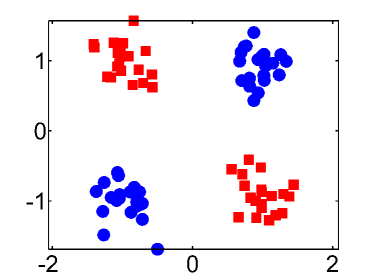
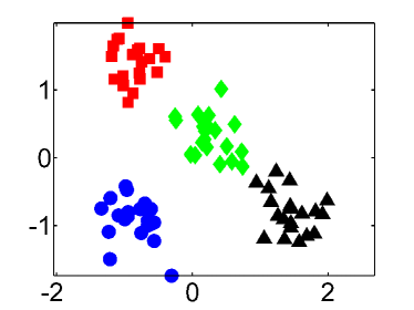
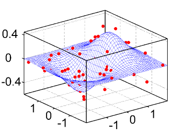
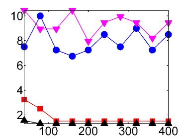
We constructed 3 artificial datasets, as illustrated in Figure 1, to illustrate the difference between BAHSIC variants with linear and nonlinear kernels. Each dataset has 22 dimensions — only the first two dimensions are related to the prediction task and the rest are just Gaussian noise. These datasets are (i) Binary XOR data: samples belonging to the same class have multimodal distributions; (ii) Multiclass data: there are 4 classes but 3 of them are collinear; (iii) Nonlinear regression data: labels are related to the first two dimension of the data by , where denotes additive Gaussian noise. We compare BAHSIC to FOHSIC, Pearson’s correlation, mutual information (Zaffalon & Hutter, 2002), and RELIEF (RELIEF works only for binary problems). We aim to show that when nonlinear dependencies exist in the data, BAHSIC with nonlinear kernels is very competent in finding them.
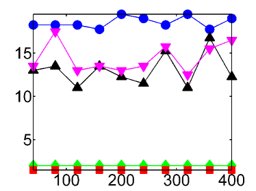
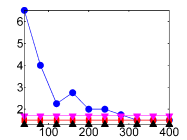
We instantiate the artificial datasets over a range of sample sizes (from 40 to 400), and plot the median rank, produced by various methods, for the first two dimensions of the data. All numbers in Figure 1 are averaged over 10 runs. In all cases, BAHSIC shows good performance. More specifically, we observe:
Binary XOR
Both BAHSIC and RELIEF correctly select the first two dimensions of the data even for small sample sizes; while FOHSIC, Pearson’s correlation, and mutual information fail. This is because the latter three evaluate the goodness of each feature independently. Hence they are unable to capture nonlinear interaction between features.
Multiclass Data
BAHSIC, FOHSIC and mutual information select the correct features irrespective of the size of the sample. Pearson’s correlation only works for large sample size. The collinearity of 3 classes provides linear correlation between the data and the labels, but due to the interference of the fourth class such correlation is picked up by Pearson’s correlation only for a large sample size.
Nonlinear Regression Data
The performance of Pearson’s correlation and mutual information is slightly better than random. BAHSIC and FOHSIC quickly converge to the correct answer as the sample size increases.
In fact, we observe that as the sample size increases, BAHSIC is able to rank the relevant features (the first two dimensions) almost correctly in the first iteration (results not shown). While this does not prove BAHSIC with nonlinear kernels is always better than that with a linear kernel, it illustrates the competence of BAHSIC in detecting nonlinear features. This is obviously useful in a real-world situations. The second advantage of BAHSIC is that it is readily applicable to both classification and regression problems, by simply choosing a different kernel on the labels.
| Data | BAHSIC | FOHSIC | PC | MI | RFE | RELIEF | R2W2 | |||||||||
|---|---|---|---|---|---|---|---|---|---|---|---|---|---|---|---|---|
| covertype | 26.3 | 1.5 | 37.9 | 1.7 | 40.3 | 1.3 | 26.7 | 1.1 | 33.0 | 1.9 | 42.7 | 0.7 | 43.4 | 0.7 | 44.2 | 1.7 |
| ionosphere | 12.3 | 1.7 | 12.8 | 1.6 | 12.3 | 1.5 | 13.1 | 1.7 | 20.2 | 2.2 | 11.7 | 2.0 | 35.9 | 0.4 | 13.7 | 2.7 |
| sonar | 27.9 | 3.1 | 25.0 | 2.3 | 25.5 | 2.4 | 26.9 | 1.9 | 21.6 | 3.4 | 24.0 | 2.4 | 36.5 | 3.3 | 32.3 | 1.8 |
| heart | 14.8 | 2.4 | 14.4 | 2.4 | 16.7 | 2.4 | 15.2 | 2.5 | 21.9 | 3.0 | 21.9 | 3.4 | 30.7 | 2.8 | 19.3 | 2.6 |
| breastcancer | 3.8 | 0.4 | 3.8 | 0.4 | 4.0 | 0.4 | 3.5 | 0.5 | 3.4 | 0.6 | 3.1 | 0.3 | 32.7 | 2.3 | 3.4 | 0.4 |
| australian | 14.3 | 1.3 | 14.3 | 1.3 | 14.5 | 1.3 | 14.5 | 1.3 | 14.8 | 1.2 | 14.5 | 1.3 | 35.9 | 1.0 | 14.5 | 1.3 |
| splice | 22.6 | 1.1 | 22.6 | 1.1 | 22.8 | 0.9 | 21.9 | 1.0 | 20.7 | 1.0 | 22.3 | 1.0 | 45.2 | 1.2 | 24.0 | 1.0 |
| svmguide3 | 20.8 | 0.6 | 20.9 | 0.6 | 21.2 | 0.6 | 20.4 | 0.7 | 21.0 | 0.7 | 21.6 | 0.4 | 23.3 | 0.3 | 23.9 | 0.2 |
| adult | 24.8 | 0.2 | 24.4 | 0.6 | 18.3 | 1.1 | 21.6 | 1.1 | 21.3 | 0.9 | 24.4 | 0.2 | 24.7 | 0.1 | 100.0 | 0.0∗ |
| cleveland | 19.0 | 2.1 | 20.5 | 1.9 | 21.9 | 1.7 | 19.5 | 2.2 | 20.9 | 2.1 | 22.4 | 2.5 | 25.2 | 0.6 | 21.5 | 1.3 |
| derm | 0.3 | 0.3 | 0.3 | 0.3 | 0.3 | 0.3 | 0.3 | 0.3 | 0.3 | 0.3 | 0.3 | 0.3 | 24.3 | 2.6 | 0.3 | 0.3 |
| hepatitis | 13.8 | 3.5 | 15.0 | 2.5 | 15.0 | 4.1 | 15.0 | 4.1 | 15.0 | 2.5 | 17.5 | 2.0 | 16.3 | 1.9 | 17.5 | 2.0 |
| musk | 29.9 | 2.5 | 29.6 | 1.8 | 26.9 | 2.0 | 31.9 | 2.0 | 34.7 | 2.5 | 27.7 | 1.6 | 42.6 | 2.2 | 36.4 | 2.4 |
| optdigits | 0.5 | 0.2 | 0.5 | 0.2 | 0.5 | 0.2 | 3.4 | 0.6 | 3.0 | 1.6 | 0.9 | 0.3 | 12.5 | 1.7 | 0.8 | 0.3 |
| specft | 20.0 | 2.8 | 20.0 | 2.8 | 18.8 | 3.4 | 18.8 | 3.4 | 37.5 | 6.7 | 26.3 | 3.5 | 36.3 | 4.4 | 31.3 | 3.4 |
| wdbc | 5.3 | 0.6 | 5.3 | 0.6 | 5.3 | 0.7 | 6.7 | 0.5 | 7.7 | 1.8 | 7.2 | 1.0 | 16.7 | 2.7 | 6.8 | 1.2 |
| wine | 1.7 | 1.1 | 1.7 | 1.1 | 1.7 | 1.1 | 1.7 | 1.1 | 3.4 | 1.4 | 4.2 | 1.9 | 25.1 | 7.2 | 1.7 | 1.1 |
| german | 29.2 | 1.9 | 29.2 | 1.8 | 26.2 | 1.5 | 26.2 | 1.7 | 27.2 | 2.4 | 33.2 | 1.1 | 32.0 | 0.0 | 24.8 | 1.4 |
| gisette | 12.4 | 1.0 | 13.0 | 0.9 | 16.0 | 0.7 | 50.0 | 0.0 | 42.8 | 1.3 | 16.7 | 0.6 | 42.7 | 0.7 | 100.0 | 0.0∗ |
| arcene | 22.0 | 5.1 | 19.0 | 3.1 | 31.0 | 3.5 | 45.0 | 2.7 | 34.0 | 4.5 | 30.0 | 3.9 | 46.0 | 6.2 | 32.0 | 5.5 |
| madelon | 37.9 | 0.8 | 38.0 | 0.7 | 38.4 | 0.6 | 51.6 | 1.0 | 41.5 | 0.8 | 38.6 | 0.7 | 51.3 | 1.1 | 100.0 | 0.0∗ |
| 11.2 | 14.8 | 19.7 | 48.6 | 42.2 | 25.9 | 85.0 | 138.3 | |||||||||
| satimage | 15.8 | 1.0 | 17.9 | 0.8 | 52.6 | 1.7 | 22.7 | 0.9 | 18.7 | 1.3 | - | 22.1 | 1.8 | - | ||
| segment | 28.6 | 1.3 | 33.9 | 0.9 | 22.9 | 0.5 | 27.1 | 1.3 | 24.5 | 0.8 | - | 68.7 | 7.1 | - | ||
| vehicle | 36.4 | 1.5 | 48.7 | 2.2 | 42.8 | 1.4 | 45.8 | 2.5 | 35.7 | 1.3 | - | 40.7 | 1.4 | - | ||
| svmguide2 | 22.8 | 2.7 | 22.2 | 2.8 | 26.4 | 2.5 | 27.4 | 1.6 | 35.6 | 1.3 | - | 34.5 | 1.7 | - | ||
| vowel | 44.7 | 2.0 | 44.7 | 2.0 | 48.1 | 2.0 | 45.4 | 2.2 | 51.9 | 2.0 | - | 85.6 | 1.0 | - | ||
| usps | 43.4 | 1.3 | 43.4 | 1.3 | 73.7 | 2.2 | 67.8 | 1.8 | 55.8 | 2.6 | - | 67.0 | 2.2 | - | ||
| housing | 18.5 | 2.6 | 18.9 | 3.6 | 25.3 | 2.5 | 18.9 | 2.7 | - | - | - | - | ||||
| bodyfat | 3.5 | 2.5 | 3.5 | 2.5 | 3.4 | 2.5 | 3.4 | 2.5 | - | - | - | - | ||||
| abalone | 55.1 | 2.7 | 55.9 | 2.9 | 54.2 | 3.3 | 56.5 | 2.6 | - | - | - | - | ||||
6.2 Real world datasets
Algorithms
In this experiment, we show that the performance of BAHSIC can be comparable to other state-of-the-art feature selectors, namely SVM Recursive Feature Elimination (RFE) (Guyon et al., 2002), RELIEF (Kira & Rendell, 1992), -norm SVM () (Weston et al., 2003), and R2W2 (Weston et al., 2000). We used the implementation of these algorithms as given in the Spider machine learning toolbox, since those were the only publicly available implementations.111http://www.kyb.tuebingen.mpg.de/bs/people/spider Furthermore, we also include filter methods, namely FOHSIC, Pearson’s correlation (PC), and mutual information (MI), in our comparisons.
Datasets
We used various real world datasets taken from the UCI repository,222http://www.ics.uci.edu/~mlearn/MLSummary.html the Statlib repository,333http://lib.stat.cmu.edu/datasets/ the LibSVM website,444http://www.csie.ntu.edu.tw/~cjlin/libsvmtools/datasets/ and the NIPS feature selection challenge555http://clopinet.com/isabelle/Projects/NIPS2003/ for comparison. Due to scalability issues in Spider, we produced a balanced random sample of size less than 2000 for datasets with more than 2000 samples.
Experimental Protocol
We report the performance of an SVM using a Gaussian kernel on a feature subset of size 5 and 10-fold cross-validation. These 5 features were selected per fold using different methods. Since we are comparing the selected features, we used the same SVM for all methods: a Gaussian kernel with set as the median distance between points in the sample (Schölkopf & Smola, 2002) and regularization parameter . On classification datasets, we measured the performance using the error rate, and on regression datasets we used the percentage of variance not-explained (also known as ). The results for binary datasets are summarized in the first part of Table 1. Those for multiclass and regression datasets are reported respectively in the second and the third parts of Table 1.
To provide a concise summary of the performance of various methods on binary datasets, we measured how the methods compare with the best performing one in each dataset in Table 1. We recorded the best absolute performance of all feature selectors as the baseline, and computed the distance of each algorithm to the best possible result. In this context it makes sense to penalize catastrophic failures more than small deviations. In other words, we would like to have a method which is at least almost always very close to the best performing one. Taking the distance achieves this effect, by penalizing larger differences more heavily. It is also our goal to choose an algorithm that performs homogeneously well across all datasets. The distance scores are listed for the binary datasets in Table 1. In general, the smaller the distance, the better the method. In this respect, BAHSIC and FOHSIC have the best performance. We did not produce the distance for multiclass and regression datasets, since the limited number of such datasets did not allow us to draw statistically significant conclusions.
| Subject | aa | al | av | aw | ay | |||||
|---|---|---|---|---|---|---|---|---|---|---|
| CSP | 17.5 | 2.5 | 3.1 | 1.2 | 32.1 | 2.5 | 7.3 | 2.7 | 6.0 | 1.6 |
| CSSP | 14.9 | 2.9 | 2.4 | 1.3 | 33.0 | 2.7 | 5.4 | 1.9 | 6.2 | 1.5 |
| CSSSP | 12.2 | 2.1 | 2.2 | 0.9 | 31.8 | 2.8 | 6.3 | 1.8 | 12.7 | 2.0 |
| BAHSIC | 13.7 | 4.3 | 1.9 | 1.3 | 30.5 | 3.3 | 6.1 | 3.8 | 9.0 | 6.0 |
6.3 Brain-computer interface dataset
In this experiment, we show that BAHSIC selects features that are meaningful in practise: we use BAHSIC to select a frequency band for a brain-computer interface (BCI) data set from the Berlin BCI group (Dornhege et al., 2004). The data contains EEG signals (118 channels, sampled at 100 Hz) from five healthy subjects (‘aa’, ‘al’, ‘av’, ‘aw’ and ‘ay’) recorded during two types of motor imaginations. The task is to classify the imagination for individual trials.
Our experiment proceeded in 3 steps: (i) A Fast Fourier transformation (FFT) was performed on each channel and the power spectrum was computed. (ii) The power spectra from all channels were averaged to obtain a single spectrum for each trial. (iii) BAHSIC was used to select the top 5 discriminative frequency components based on the power spectrum. The 5 selected frequencies and their 4 nearest neighbours were used to reconstruct the temporal signals (with all other Fourier coefficients eliminated). The result was then passed to a normal CSP method (Dornhege et al., 2004) for feature extraction, and then classified using a linear SVM.
We compared automatic filtering using BAHSIC to other filtering approaches: normal CSP method with manual filtering (8-40 Hz), the CSSP method (Lemm et al., 2005), and the CSSSP method (Dornhege et al., 2006). All results presented in Table 2 are obtained using -fold cross-validation. Our method is very competitive and obtains the first and second place for 4 of the 5 subjects. While the CSSP and the CSSSP methods are specialised embedded methods (w.r.t. the CSP method) for frequency selection on BCI data, our method is entirely generic: BAHSIC decouples feature selection from CSP.
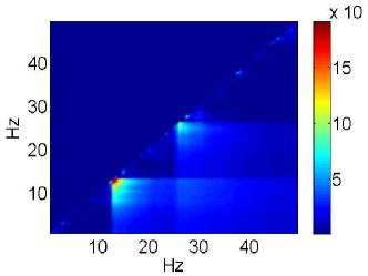
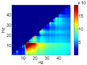
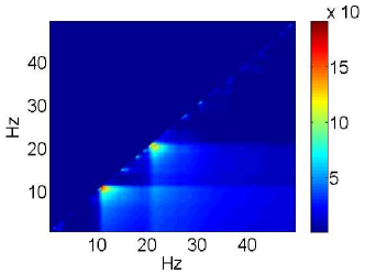
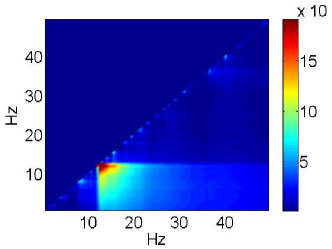
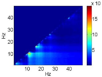
In Figure 2, we use HSIC to visualise the responsiveness of different frequency bands to motor imagination. The horizontal and the vertical axes in each subfigure represent the lower and upper bounds for a frequency band, respectively. HSIC is computed for each of these bands. (Dornhege et al., 2006) report that the rhythm (approx. 12 Hz) of EEG is most responsive to motor imagination, and that the rhythm (approx. 22 Hz) is also responsive. We expect that HSIC will create a strong peak at the rhythm and a weaker peak at the rhythm, and the absence of other responsive frequency components will create block patterns. Both predictions are confirmed in Figure 2. Furthermore, the large area of the red region for subject ‘al’ indicates good responsiveness of his rhythm. This also corresponds well with the lowest classification error obtained for him in Table 2.
7 Conclusion
This paper proposes a backward elimination procedure for feature selection using the Hilbert-Schmidt Independence Criterion (HSIC). The idea behind the resulting algorithm, BAHSIC, is to choose the feature subset that maximises the dependence between the data and labels. With this interpretation, BAHSIC provides a unified feature selection framework for any form of supervised learning. The absence of bias and good convergence properties of the empirical HSIC estimate provide a strong theoretical jutification for using HSIC in this context. Although BAHSIC is a filter method, it still demonstrates good performance compared with more specialised methods in both artificial and real world data. It is also very competitive in terms of runtime performance.666Code is freely available as part of the Elefant package at http://elefant.developer.nicta.com.au.
Acknowledgments
NICTA is funded through the Australian Government’s Baking Australia’s Ability initiative, in part through the ARC.This research was supported by the Pascal Network (IST-2002-506778).
Appendix
Theorem 1.
Recall that . We prove the claim by constructing unbiased estimators for each term in (3). Note that we have three types of expectations, namely , a partially decoupled expectation , and , which takes all four expectations independently.
If we want to replace the expectations by empirical averages, we need to take care to avoid using the same discrete indices more than once for independent random variables. In other words, when taking expectations over independent random variables, we need -tuples of indices where each index occurs exactly once. The sets satisfy this property. Their cardinalities are given by the Pochhammer symbols . Jointly drawn random variables, on the other hand, share the same index. We have
In the case of the expectation over three independent terms we obtain
For four independent random variables ,
To obtain an expression for we only need to take linear combinations using (3). Collecting terms related to , , and yields
This is the expected value of . ∎
Theorem 3.
We first relate a biased estimator of HSIC to the biased estimator of MMD. The former is given by
and the bias is bounded by , as shown by (Gretton et al., 2005). An estimator of MMD with bias is
If we choose with and , we can see . In this case , which shows that the biased estimators of MMD and HSIC are identical up to a constant factor. Since the bias of is , this implies the same bias for the MMD estimate.
To see the same result for Kernel Target Alignment, note that for equal class size the normalisations with regard to and become irrelevant, which yields the corresponding MMD term. ∎
References
- Baker (1973) Baker, C. (1973). Joint measures and cross-covariance operators. Transactions of the American Mathematical Society, 186, 273–289.
- Borgwardt et al. (2006) Borgwardt, K. M., Gretton, A., Rasch, M. J., Kriegel, H.-P., Schölkopf, B., & Smola, A. J. (2006). Integrating structured biological data by kernel maximum mean discrepancy. Bioinformatics (ISMB), 22(14), e49–e57.
- Cristianini et al. (2003) Cristianini, N., Kandola, J., Elisseeff, A., & Shawe-Taylor, J. (2003). On optimizing kernel alignment. Tech. rep., UC Davis Department of Statistics.
- Dornhege et al. (2004) Dornhege, G., Blankertz, B., Curio, G., & Müller, K. (2004). Boosting bit rates in non-invasive EEG single-trial classifications by feature combination and multi-class paradigms. IEEE Trans. Biomed. Eng., 51, 993–1002.
- Dornhege et al. (2006) Dornhege, G., Blankertz, B., Krauledat, M., Losch, F., Curio, G., & Müller, K. (2006). Optimizing spatio-temporal filters for improving BCI. In NIPS, vol. 18.
- Fukumizu et al. (2004) Fukumizu, K., Bach, F. R., & Jordan, M. I. (2004). Dimensionality reduction for supervised learning with reproducing kernel hilbert spaces. JMLR, 5, 73–99.
- Gretton et al. (2005) Gretton, A., Bousquet, O., Smola, A., & Schölkopf, B. (2005). Measuring statistical dependence with Hilbert-Schmidt norms. In ALT, 63–78.
- Guyon & Elisseeff (2003) Guyon, I., & Elisseeff, A. (2003). An introduction to variable and feature selection. Journal of Machine Learning Research, 3, 1157–1182.
- Guyon et al. (2002) Guyon, I., Weston, J., Barnhill, S., & Vapnik, V. (2002). Gene selection for cancer classification using support vector machines. Machine Learning, 46, 389–422.
- Kira & Rendell (1992) Kira, K., & Rendell, L. (1992). A practical approach to feature selection. In Proc. 9th Intl. Workshop on Machine Learning, 249–256.
- Koller & Sahami (1996) Koller, D., & Sahami, M. (1996). Toward optimal feature selection. In ICML, 284–292.
- Lemm et al. (2005) Lemm, S., Blankertz, B., Curio, G., & Mülller, K.-R. (2005). Spatio-spectral filters for improving the classification of single trial EEG. IEEE Trans. Biomed. Eng., 52, 1541–1548.
- Nemenman et al. (2002) Nemenman, I., Shafee, F., & Bialek, W. (2002). Entropy and inference, revisited. In NIPS, vol. 14.
- Neumann et al. (2005) Neumann, J., Schnörr, C., & Steidl, G. (2005). Combined SVM-based feature selection and classification. Machine Learning, 61, 129–150.
- Schölkopf & Smola (2002) Schölkopf, B., & Smola, A. (2002). Learning with Kernels. Cambridge, MA: MIT Press.
- Serfling (1980) Serfling, R. (1980). Approximation Theorems of Mathematical Statistics. New York: Wiley.
- Steinwart (2002) Steinwart, I. (2002). On the influence of the kernel on the consistency of svms. JMLR, 2, 67–93.
- Weston et al. (2003) Weston, J., Elisseeff, A., Schölkopf, B., & Tipping, M. (2003). Use of zero-norm with linear models and kernel methods. JMLR, 3, 1439–1461.
- Weston et al. (2000) Weston, J., Mukherjee, S., Chapelle, O., Pontil, M., Poggio, T., & Vapnik, V. (2000). Feature selection for SVMs. In NIPS, vol. 13.
- Zaffalon & Hutter (2002) Zaffalon, M., & Hutter, M. (2002). Robust feature selection using distributions of mutual information. In UAI.