Gems: Galaxy fitting catalogues and testing
parametric galaxy fitting codes:
Galfit, Gim2d
Abstract
In the context of measuring structure and morphology of intermediate redshift galaxies with recent HST/ACS surveys, we tune, test, and compare two widely used fitting codes (Galfit and Gim2d) for fitting single-component Sérsic models to the light profiles of both simulated and real galaxy data. Our study focuses on the Gems survey with the sensitivity of typical HST survey data, and we include our final catalog of fit results for all 41,495 objects detected in Gems. We test the reliability of both codes using simulated galaxy profiles constructed to represent the imaging characteristics of Gems. We find that fitting accuracy depends sensitively on galaxy profile shape. Exponential disks are well fit with Sérsic models and have small measurement errors, whereas fits to de Vaucouleurs profiles show larger uncertainties owing to the large amount of light at large radii. We find that both codes provide reliable fits and little systematic error, when the effective surface brightness is above that of the sky. Moreover, both codes return errors that significantly underestimate the true fitting uncertainties, which are best estimated with simulations. We find that Gim2d suffers significant systematic errors for spheroids with close companions owing to the difficulty of effectively masking out neighboring galaxy light; there appears to be no work around to this important systematic in Gim2d’s current implementation. While this crowding error affects only a small fraction of galaxies in Gems, it must be accounted for in the analysis of deeper cosmological images or of more crowded fields with Gim2d. In contrast, Galfit results are robust to the presence of neighbors because it can simultaneously fit the profiles of multiple companions thereby deblending their effect on the fit to the galaxy of interest. We find Galfit’s robustness to nearby companions and factor of faster runtime speed are important advantages over GIM2D for analyzing large HST/ACS datasets.
Subject headings:
methods: data analysis — catalogs — surveys — galaxies: general — galaxies: photometry — galaxies: statistics1. Introduction
One of the central goals of observational exploration of galaxy evolution is to understand how the structures of galaxies evolve with cosmic time. A powerful tool in this context are large look-back surveys, where the time evolution of the distribution of galaxy structural properties can be quantified. The key to unlocking the potential of these surveys is the development of quantifiable, well-understood, and repeatable ways to measure and describe galaxy structures. Using such methods, the evolution of the structure of disk galaxies (Lilly, 1998; Simard & Pritchet, 1998; Ravindranath et al., 2004; Barden et al., 2005; Trujillo & Pohlen, 2005; Sargent et al., 2006) and spheroid-dominated galaxies (e.g., Schade et al., 1997, 1999; McIntosh et al., 2005; Trujillo et al., 2004, 2006) has been quantified over the last 10 billion years of cosmic time, since . In this paper, we exhaustively test and tune two parametric galaxy fitting codes, Galfit (Peng et al., 2002) and Gim2d (Simard, 2002), that are commonly used in the literature. With these tests we determine the best fitting setups for each code, quantify the sources of random and systematic uncertainty, and presents parametric fits for 41,495 objects in the HST Gems (Rix et al., 2004) dataset.
There are two main approaches towards describing galaxy structure from the two-dimensional information contained in image data. Non-parametric methods provide estimates of total brightness, galaxy half-light size, and structure, using metrics which do not depend on a galaxy, having a structure well-described by any particular functional form (e.g., Petrosian, 1976; Abraham et al., 1996; Bershady, Jangren & Conselice, 2000; Lotz et al., 2006). The main disadvantages of non-parametric methods are that they are reasonably sensitive to the depth of the images; because there is no parametric form for extrapolating to account for the faint outer parts of galaxies, one can underestimate flux and/or size in poorly-posed cases (Blanton et al., 2003). Parametric methods, in contrast, choose particular functional forms (sometimes reasonably complicated) with which to fit the galaxy light distribution. These have substantially less flexibility than non-parametric fitting codes, but have the advantage that light at large radii can be accounted for reasonably well by the natural extrapolation of the best-fitting model profile (under the assumption that the parametric form chosen does, in fact, describe the light profile in the outer parts of galaxies reasonably well). Besides robust estimates of galaxy size, parametric methods provide measures of galaxy structure that may shed light on relative contributions of physically distinct and meaningful components such as spheroids, disks, and stellar bars.
One particularly useful and flexible profile for parametric galaxy fitting is a single-component Sérsic (1968) model, which describes the radial surface brightness profile of a galaxy by the Sérsic function given by
| (1) |
where is the radius of the galaxy (Note that for a Sérsic fit is equivalent to the half-light radius ), is the surface brightness at , and the Sérsic parameter describes the profile shape (the parameter is closely connected to ). Together with position (x and y), axis ratio and position angle, this profile has 7 free parameters. The Sérsic profile represents a more general form of the exponential light-profiles seen in galactic disks () and the -law (de Vaucouleurs law) profiles typical of luminous early-type galaxy () (e.g., deVaucouleurs, 1948; Freeman, 1970); fitting with this profile has been explored in detail in a number of works (e.g., Simard, 1998, 2002; Graham et al., 2005; Trujillo et al., 2001). Figure 1 shows some examples of Sérsic profiles with different . Many authors have used a constant value of or to crudely distinguish early-type (bulge-dominated) from late-type (disk-dominated) galaxies (e.g., Blanton et al., 2003; Shen et al., 2003; Hogg et al., 2004; Bell et al., 2004; Barden et al., 2005; McIntosh et al., 2005; Ravindranath et al., 2004). Furthermore, fitting galaxies with a Sérsic profile gives an estimate of size, and therefore is very useful for the examination of the evolution of galaxy scaling relations.
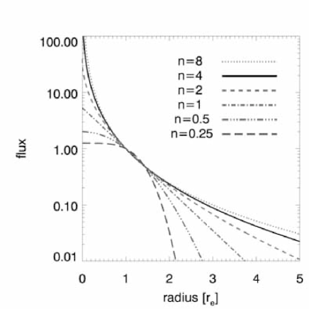
The goal of this paper is to describe our efforts to optimize the estimation of single-component Sérsic profile fits to the galaxies in the Gems survey (Rix et al., 2004). To date, this has been our primary method for quantifying galaxy structure111Bulge-disk composite galaxies were not simulated for this paper; bulge-disk decomposition will be addressed in a future paper.. We compare the performance of the Galfit and Gim2d automated galaxy fitting codes, which are suitable for fitting large datasets such as Gems, Stages (Gray et al., , in prep.), Goods (Giavalisco et al., 2004) and Cosmos (Scoville et al., ). We address the reliability and limitations of these codes through thorough testing, using simulated and real galaxies. We describe the details of the simulations used throughout this paper in §2. In §3 we explore different set-ups, converging on ‘best-fitting’ set-ups for each fitting code. §4 summarizes the results from our testing of these ‘best-fitting’ set-ups using both simulated galaxies (§4.1 and §4.2) and real galaxies (§4.3). We compare our findings with those of a recent paper on the same topic (using the codes Galfit, Gim2d, and Gasphot) by Pignatelli et al. (2006) in §5, and publish a catalog of Galfit fitting results for all 41,495 detected galaxies from the Gems survey in §6. All results from this paper and a number of other catalogs and images useful for testing galaxy fitting codes are presented on the Gems webpage222see http://www.mpia.de/GEMS/gems.htm.
2. Simulations
Galaxy simulations are an invaluable tool for understanding the performance of quantitative fitting pipelines. In this section we describe the set of simulations that are extensively used for this paper; the results obtained from fitting these simulations are discussed in §4.
In this paper, we focus on simulations of two different galaxy light profiles: purely exponential profiles () representing the luminosity profile of a galactic disk (we will call these galaxies ‘disks’ throughout this paper), and Sérsic profiles with a Sérsic index of representing a de Vaucouleurs luminosity profile of a galactic bulge/elliptical galaxy (we will call them ‘spheroids’), respectively. Profiles having Sérsic indices between these two values of 1 and 4 are not presented here because and simulations span the range of observed behavior, exponential profiles being the ‘easiest’ to fit, de Vaucouleurs being the ‘hardest’. Nonetheless, extensive simulations of intermediate profiles (200,000 objects) have been produced, the catalog of Galfit fitting results for this sample can also be downloaded from the Gems webpage.
This section is arranged as follows. The simulation of individual galaxies is described in §2.1. Section 2.2 describes the construction of simulated Gems frames from the individual galaxy simulations, including the addition of realistic noise.
2.1. Simulation of individual noise-free galaxies & Oversampling
Galaxies were simulated using a custom-built IDL routine. Most available standard
routines (like MKOBJECT in IRAF, create/image in MIDAS
and similar tasks in other programs) compute the correct flux value for the center of the pixel, but due to curvature of the profile, taking this as the mean
flux value for the whole pixel is incorrect. The higher the curvature is
(within a certain pixel), the more one underestimates the true pixel value. This
implies progressively larger inaccuracies for higher Sérsic indices.
While it is possible to analytically integrate the profile across a pixel to obtain
an exact answer, this procedure is very CPU-intensive. We adopt a hybrid approach.
We use IDL’s dist_ellipse routine in conjunction with equation
(1) to compute Sérsic galaxy models which, as in the above cases, are
only correct for the center of the pixel. In order to increase accuracy, the inner
parts of our simulated profiles (100x100 pixels up to 200x200 pixels depending on
object size) have been oversampled by a factor of 10, and the very inner parts
(10x10 up to 20x20 pixels) are oversampled by a factor of 100. This was done by
creating the images by a factor of 10 (or 100 respectively) bigger and then
rebinning the image while holding the total flux constant. In this way, it is
possible to create a final profile accurate to better than 0.03% at all radii (much
smaller than the poisson noise added later in the simulation process) with a factor
of 100 gain in speed compared to the analytical integration – an important gain
when simulating large samples of galaxies.
2.2. Simulation of crowded images
To realistically test galaxy extraction and fitting codes requires the creation of images with large numbers of simulated galaxies distributed as in real data. Such images were created by providing a catalog of simulated galaxy input parameters to the simulation code, which simulated galaxies at the location, luminosity, size, orientation and axis ratio specified in this catalog. In this step, galaxies were put in an empty image of the same size as the final image.
| Parameter | Min | Max | Distribution |
|---|---|---|---|
| mag [mag] | 20 | 26.5 | uniform |
| [pixel] | 2 | 316 | uniform in logarithmic space |
| , mag being chosen magnitude for object | |||
| 0.18 | 1 | uniform in , being inclination angle | |
| corrected for intrinsic thickness: | |||
| intrinsic thickness 0.18 following Pizagno et al. (2005); Ryden (2006) and others | |||
| PA [deg to image] | 0 | 180 | uniform |
| Sérsic index | 1 | 1 | fixed |
| Parameter | Min | Max | Distribution |
|---|---|---|---|
| mag [mag] | 20 | 27 | uniform |
| [pixel] | 2 | 630 | uniform in logarithmic space |
| 0.45 | 1 | uniform in , being inclination angle | |
| corrected for intrinsic thickness: | |||
| PA [deg to image] | 0 | 180 | uniform |
| Sérsic index | 4 | 4 | fixed |
To choose the range of galaxy parameters for the simulated galaxies, we first fitted all Gems galaxies with Galfit and determined the parameter range covered by the real galaxy sample. Given these results, we chose a wider range of parameter space for the simulations, in order to test detection efficiency, completeness, and to allow pushing both parametric fitting codes to their limits. The simulations have a random distribution in size between 2 and 316 pixels (uniformly distributed in logarithmic space) and magnitude between 20 and 27 (uniform). With this distribution of parameters, there were a relatively large number of large and low surface brightness galaxies (stringently testing the detection efficiency and fitting codes); we discuss this point in more detail in §4.2. The exact distributions of simulation parameters are given in Tables 1 and 2.
After simulating the galaxy profiles and putting them in an empty image, this final image was convolved with a real F850LP-band PSF derived from the Gems dataset (Jahnke et al., 2004). Next, an appropriate amount of noise had to be added to the images. Owing to the multiple-frame dither characteristic of HST imaging surveys, the noise is somewhat correlated pixel-to-pixel. Thus, strictly speaking, galaxies should be simulated in individual dithers, then dithered together using exactly the same routines as were used to combine the Gems frames. We took an intermediate approach: Poisson noise with the same RMS as the Gems noise was added to the simulated galaxy frame, then a real ‘sky’ frame was added to the simulated frame to accurately account for real fluctuations and correlated noise in observed HST sky backgrounds. We have confirmed through tests with Galfit that this (much less CPU- and work-intensive) hybrid approach yields a scatter which is negligible compared to random fitting uncertainties. The ‘sky’ frame was constructed by adding Gems F606W- and F850LP-band frames (to increase image depth and to make sure that objects appear in neither of the two bands) and visually checking those images to identify patches of 500x500 pixels in size without objects detected by SExtractor. The chosen patches were cut from the F850LP-band images and pasted together to form an empty image of the same size as an original Gems image.
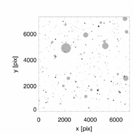
The result of the simulation process was a simulated image with noise properties very similar to a real Gems image that contained 800 simulated light profiles with different magnitudes, sizes, position angles and values of . Different sets of simulations were created in this way: one set contains disk-like galaxies only (for results see §4.1.1) and the other contains spheroidal profiles only (see §4.1.2). Not all 800 galaxies were recovered by SExtractor. Roughly 80% of the objects were recovered, depending on the simulated profile shape and the distribution of galaxy parameters in the particular image (see Figure 2). In particular, very large and low surface-brightness galaxies were not detected (see Figure 2 and Rix et al., 2004). Due to the fact that spheroids are easier to detect due to their centrally concentrated light profiles, less galaxies were recovered in the disk sample.
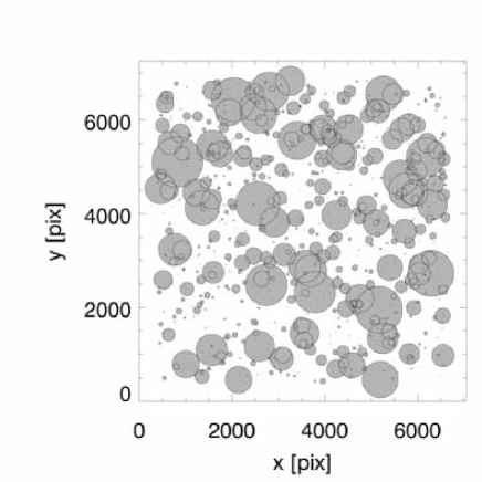
By design, these simulated tiles are artificial in two ways. Firstly, the galaxy input parameters span a wider range in parameter space than real galaxies. Secondly, the simulated tiles are significantly more crowded than the actual data itself, about a factor of 7–8 overdense in galaxies with Sérsic index compared to a typical ACS image from Gems (see Figure 3). They contain many more LSB galaxies (detected and undetected), adding a complex layer of extra flux to the background. This makes the simulations more difficult to analyze than real data; this was intentional since we wanted to push both codes to their limits. In a third set of simulations we mixed the two types of profile (see §4.2) to estimate the effects of deblending given a more realistic mix of and galaxies.
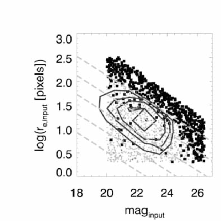
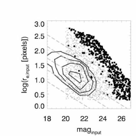
To test and compare the two different 2D-fitting routines, the simulated images were treated as ‘real’ images, i.e. we used exactly the same data pipeline for fitting that was used for the real Gems data analysis. Therefore, all effects which we can see in the results from simulations should be present in real data as well, although mixed with many other effects like bulge/disk composite profiles, non-smoothness, lumpiness and/or spiral features of real galaxies.
3. Galaxy fitting: Description, Basic Considerations, Best-fitting Setups
For the Gems analysis, we have used two widely-employed parametric fitting codes for quantitatively describing galaxy structure and morphology: Galfit and Gim2d. In this section, we describe both codes and the procedures used to parametrically fit both the real Gems data and the simulations described in the previous section. The basic considerations for code setup and application to real data, and the tests which we have performed on simulated data, are useful in general to other workers in galaxy image fitting. These basic considerations for setup and application of these (and most) fitting codes are (1) sky estimation, (2) initial parameter guesses, (3) postage stamp construction, and (4) deblending and/or masking of neighboring sources. We describe in detail the setups and various tests we carried out in order to optimize these setups in §3.1 for Galfit and §3.2 for Gim2d.
The initial conditions and setups for both Galfit and Gim2d are determined using SExtractor output images and catalogues. We use SExtractor (version 2.2.2 , Bertin & Arnouts, 1996) for image parsing and catalog creation. SExtractor detects, deblends, measures and classifies objects, giving estimates of magnitude, size, , position angle and a star-galaxy classification. In Gems, we found that no single SExtractor setup satisfactorily detected and deblended both bright, well-resolved galaxies and faint galaxies near the detection limit. Accordingly, our best setup is to run SExtractor twice: once to detect the bright objects without splitting them up (what we call the ‘cold’ version) and once to detect the faint objects (‘hot’ version). The two versions are then combined to give one single catalog containing all objects. The procedure is described in more detail in Rix et al. (2004) and Caldwell et al. (2006). We do not use the SExtractor output catalogs directly for science; instead, these values are used as initial estimates for galaxy fitting codes and their setup. In the following sections we will describe which parameters are taken as starting guesses and how these values are used for the two parametric galaxy fitting codes used in this work: Galfit and Gim2d.
3.1. GALFIT
Galfit is a 2D galaxy fitting software package written by Peng et al. (2002). We used Galfit Version 2.0.3b from Feb. 2, 2005 for this analysis. Galfit was designed to extract structural components from galaxy images. Compared to other fitting techniques it has two main advantages. It uses a Levenberg-Marquardt downhill-gradient (Press, 1997) method to derive the best fit and therefore is relatively fast, being able to fit roughly 3000 galaxies per day on a dual 2.4 GHz LINUX processor (when running 4 threads simultaneously to efficiently use all CPU time). Furthermore, due to its speed and design, it is able to fit an image containing an arbitrary number of galaxies simultaneously, making it possible to fit neighboring objects. The main disadvantage of Galfit, in theory, is that it is possible that it converges on fit solutions that represent a local minimum instead of giving the global minimum. Our experience with Galfit is that in single component, but multi-object, fits this happens relatively rarely, if at all, both through the simulations (§4.1) and through comparison of fitting results for real galaxies from Galfit and Gim2d (§4.3).
During the fitting process, the model is convolved with a specified PSF to model the image seeing and then compared to the input image. It is possible to fit the background sky level during the fitting process, although in this paper we use this capability for testing purposes only (see §3.1.2).
In the following section, we will explain the basic setup procedure of Galfit in detail; e.g., cutting postage stamps, estimating the sky background, deciding on how galaxies should be deblended, and setting up the initial parameters for Galfit. We developed automated routines for this purpose, and we describe their most important features in this section. As sky background is of critical importance, we discuss this issue in some detail in §3.1.2.
3.1.1 Galfit setup and Galapagos
Galfit is designed to fit one galaxy of interest at a time. Therefore, we created an individual postage stamp for each galaxy of interest . These postage stamps were created, and initial Galfit parameter files produced, by an IDL program, Galapagos (Galaxy Analysis over Large Areas: Parameter Assessment by Galfitting Objects from SExtractor, for further details about Galapagos and details of the procedure see Barden et al., in prep.). For every object in the SExtractor catalog Galapagos did the following.
-
1.
First, Galapagos determined the size of the required postage stamp for each object. This was done using different object sizes and angles given by SExtractor:
(2) (3) where is the SExtractor output parameter
A_IMAGE,kronisKRON_RADIUS, isTHETA_IMAGEandellipisELLIPTICITY. Extensive testing showed that this algorithm for producing postage stamps was a good compromise between the conflicting needs of having enough sky pixels present in the postage stamp to give a robust fit of the object, while keeping the postage stamps small enough to be fit in reasonable amounts of CPU time. -
2.
In the next step, Galapagos decided from this postage stamp and the aperture map, which secondary objects had to be deblended and fitted simultaneously and which objects were simply masked out during the fitting process. For this it created a second map where SExtractor aperture ellipses were increased in linear size by a factor of 1.5 (a factor of 2.25 larger area). Every object whose ellipse overlapped with the ellipse of the primary object was fitted simultaneously using a single Sérsic profile; every other object with pixels in the postage stamp was masked out during the fit, using this expanded ellipses as the mask333In many other fitting routines the SExtractor segmentation map is used for masking; our masks are considerably more conservative.. This way time-consuming fits, with 10 or more objects to be simultaneously fitted, were avoided in most cases. In total for around 48%/31%/46% of the fits, at least one secondary object had to be taken into account (for simulations, simulations and real galaxies respectively). In the most crowded situations we find that we needed to simultaneously fit a maximum of 9/7/12 profiles.
-
3.
After this step the sky background was estimated. For this, Galapagos used the aperture map on the whole science frame (and not only the postage stamp) and estimated the mean value of all pixels that lay within 6 consecutive elliptical annuli, each with a width of 60 pixels (measured along the semi-major axis; corresponding to 1.8” using the Gems data with 0.03”/pixel). These 6 annuli partially overlap, with a spacing of 30 pixels between successive annuli. The annuli were centered on the primary fitting galaxy (pixels belonging to a secondary object were ignored in this step). The innermost area is masked out during this process (the factor of 1.5 magnified aperture ellipse enlarged by a further 30 pixels). These annuli ‘marched outward’ together in radius in steps of 30 pixels until the gradient of the mean values within the last 6 rings (180 pixels) was larger than -0.05; the change in the sky value, given that the mean Gems F850LP sky background is around 18 counts, was then well below 0.3 % within this radial range. The sky was then determined as the mean value of the outermost 6 annuli. This made the area where the sky is determined to be an ellipse between 35 and 215 pixels in semi-major axis for the smallest objects (between 15 and 30 ) and an ellipse of width of 180 pixels at around 4-6 for the bigger objects (for details see Barden et al, 2006, in prep.). We call this sky estimate the ‘isophotal sky’ in what follows, and testing shows that for fitting with Galfit the ‘isophotal sky’ provides significantly better fitting results than using sky values from, e.g., SExtractor (see §3.1.2).
-
4.
In the same step, by dividing the elliptical individual annuli into 8 octants, Galapagos was able to detect sky gradients within an annulus as a function of position angle. Such cases were relatively rare, and were due to nearby bright objects that did not reach into the postage stamp themselves (especially bright high Sérsic index objects with strong wings). Galapagos then identified these objects in the SExtractor catalog automatically and these objects were fitted simultaneously to eliminate this sky gradient (Galfit can fit profiles that are centered outside of the postage stamp). In the very rare cases that an identification was not possible although a strong gradient was present (i.e. the object lay outside of the original Gems tile), we fit an artificial object centered outside the postage stamp in the correct direction to achieve the same result. In total, 15.2% of the fits in the simulated disk sample needed an additional identified profile centered outside of the postage stamp, 1.5% needed an artificial, not identified profile (4.3%, 0.6% for simulated spheroidal galaxies). For real galaxies only 3% of the fits needed an identified object, 0.4% needed an artificial profile. Recall that the simulated images contained a large number of galaxies not recovered by SExtractor; these galaxies contributed to the background sky only. These galaxies can lead to ‘sky’ gradients found by Galapagos. This effect should be, and is, more pronounced in the sample where fewer galaxies are recovered.
Table 3Starting guesses for Galfit when using Galapagos Parameter Starting guess from SExtractor mag MAG_BEST1 - ELLIPTICITYPA THETA_IMAGE1.5 x,y the postage stamp is centered on the primary object positions of secondary objects can be derived from SExtractor -
5.
The last step for setting up Galfit was the determination of the starting guesses for the different fitting parameters from SExtractor and writing them to a Galfit start file automatically (see Table 3). We decided to fit single Sérsic profiles to all galaxies (with a starting value of 1.5 for the Sérsic index). Starting magnitudes were given by SExtractor
MAG_BEST, sizes were given usingFLUX_RADIUS(we used the formula , where isFLUX_RADIUS. This formula was determined empirically using simulations). The axis ratio was derived by taking the SExtractorELLIPTICITY, the position angle byTHETA_IMAGE. Furthermore the position of the objects within its postage stamp was required, which was directly given by the cutting process of the postage stamps (the object is centered within its postage stamp, see step 1). The parameter diskiness/boxiness in Galfit was fixed to 0 (no boxiness/diskiness) for all our fits. Furthermore, as described above, the estimated sky value from step 3 was held fixed during the fit. Each object that had to be deblended during the fitting process was included (from step 2) with its appropriate starting values; all other objects were masked out (using a mask image with the by a factor of 1.5 enlarged SExtractor apertures that tells Galfit which pixels it should use and which pixels it should ignore during the fit). Finally, the Gems PSF (see Jahnke et al., in prep.) was provided to Galfit.
We adopted a set of fitting constraints for Galfit which prevented the code from
exploring unphysical (and time-consuming) areas of parameter space. We used
, [pixels of 0.03 in size] and fixed the fit magnitude
to be within 5 mag of the SExtractor MAG_BEST.
We used exactly the same constraints for real galaxies, also using the same setup procedure. Whenever we state that Galfit fitted ‘successfully’, we mean that Galfit returned a result (it did not crash during the fit) and the fit did not run into any of the constraints given above.
3.1.2 Galfit sky test
The estimate of the sky background is of critical importance in determining parametric or non-parametric descriptions of galaxy surface brightness profiles (e.g., de Jong, 1996). While in principle it is possible to fit the sky level as an extra parameter, such a procedure requires that the surface brightness profile being used is an accurate description of the real galaxy light profiles. An alternative is to estimate the sky level as carefully as possible prior to the fit and hold it fixed.
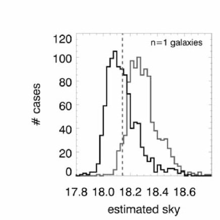
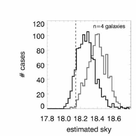
In this section we quantify the effect of different assumptions/estimates of the sky level for Galfit (the results of the equivalent test for Gim2d are shown in §3.2.3). We test three setups: i) the isophotal sky, ii) the sky value determined by SExtractor, and iii) allowing sky to be a free parameter, to be estimated by Galfit.
In Figure 4 one can see the difference between the sky values derived by the two sky estimation methods, Galapagos and SExtractor, for the two different samples of simulated =1 and =4 galaxies, respectively. Because the simulations were added to a sky frame composed of empty patches of real sky, the true sky values were known to be , indicated by the vertical dashed line in both plots. SExtractor recovers a mean value of 18.29 (=0.10) for disk galaxies and 18.40 (=0.11) for spheroidal galaxies. The isophotal estimator in Galapagos gives a mean value of 18.13 (=0.10) for disk galaxies and 18.26 (=0.11) for spheroidal galaxies. Although all distributions have around the same width, one can see that both methods recover the sky better for the low Sérsic-index sample. Furthermore, in both samples, the isophotal estimator gives back rather more accurate sky values.
That SExtractor recovers a sky value that is slightly too high has been noted before – e.g., by the Goods team444see , chapter 5.1 Local sky background and was the reason why we decided to write our own isophotal sky estimator.
That the sky is easier to estimate for the simulations than for the simulations can be partly explained by our simulation of a number of large, low surface brightness galaxies which escape detection by SExtractor and which inflate the sky surface brightness. Since galaxies with high Sérsic index have more extended wings the effect of contamination in the outskirts is larger for simulations than for . There is a further effect for galaxies: since the sky estimates provided by SExtractor and Galapagos only probe out to for brighter galaxies, there is a residual contribution to the sky from the galaxy itself which becomes more serious as increases.
| Sky used | Sérsic | ratio | ratio | Quality | |||||||
|---|---|---|---|---|---|---|---|---|---|---|---|
| mean | mean | mean | mean | mean | |||||||
| isophotal sky | 3.99 | 0.27 | 1.00 | 0.05 | 0.00 | 0.03 | 0.99 | 0.04 | 0.17 | 1.54 | 0.06 |
| SExtractor sky | 3.79 | 0.29 | 0.96 | 0.07 | 0.03 | 0.04 | 1.00 | 0.04 | 0.17 | 1.56 | 4.66 |
| Galfit sky | 3.94 | 0.24 | 0.99 | 0.06 | 0.01 | 0.03 | 1.00 | 0.04 | 0.16 | 1.55 | 0.38 |
Note. — This Table summarizes the results from using different sky estimators with Galfit for bright galaxies; see Table 5 for results for faint galaxies.
The columns give deviations (resistant mean values clipped at ) from the simulated value and scatter for the 5 key fitting parameters. The values given are values computed iteratively for all galaxies within 3 .
The last column gives the fit quality. This number is defined as:
| (4) |
where values are given as the mean values in the table. This quantity is a fairly intuitive combination of the different fit parameters, indicating in broad terms which setups perform well (low values) and which perform poorly (high values). One can see that indeed using the isophotal sky as given by Galapagos and using the sky level as a free parameter during the fit return much more reliable results than the SExtractor sky already for these bright galaxies. Using the isophotal sky seems to be the ideal setup.
| Sky used | Sérsic | ratio | ratio | Quality | |||||||
|---|---|---|---|---|---|---|---|---|---|---|---|
| mean | mean | mean | mean | mean | |||||||
| isophotal sky | 3.95 | 1.13 | 0.97 | 0.44 | 0.02 | 0.42 | 1.04 | 0.18 | 0.20 | 6.31 | 2.92 |
| SExtractor sky | 3.05 | 0.98 | 0.61 | 0.27 | 0.41 | 0.39 | 1.05 | 0.18 | -0.06 | 6.38 | 375.33 |
| Galfit sky | 3.78 | 1.16 | 0.94 | 0.47 | 0.09 | 0.44 | 1.04 | 0.19 | 0.07 | 6.12 | 16.93 |
Note. — Same as Table 4, but for faint galaxies. As one can clearly see from this table and as was expected, fitting faint galaxies is more difficult. Using the isophotal sky during the fit returns the best fitting results, slightly better than the internal estimation in Galfit. Using the SExtractor sky returns significantly worse results.
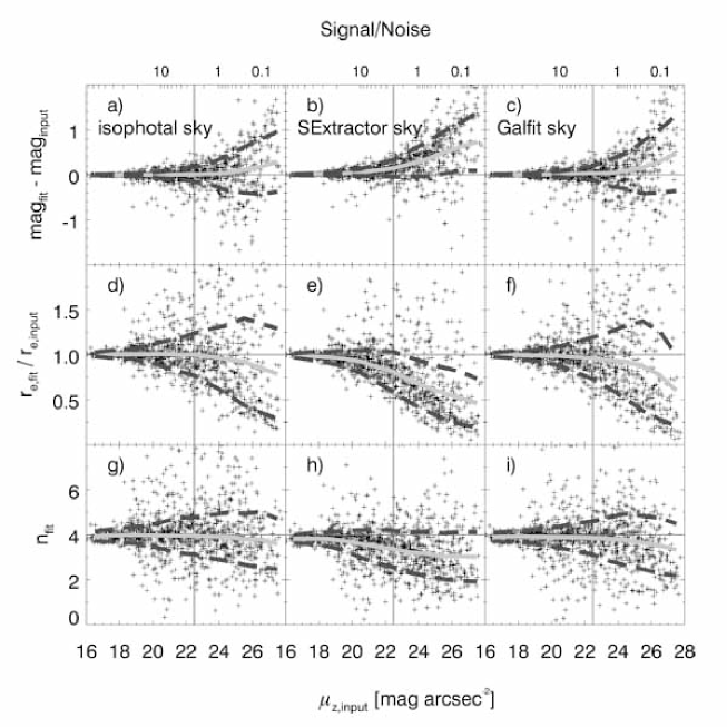
We compare the fitting results with the three different sky setups in Figure 5. We only show results for the sample of simulated galaxies; the results for the galaxies were qualitatively similar but the systematic effects are much weaker, showing very little difference between the three different sky setups. The Y-axis shows the deviation of the three key parameters magnitude, and from their true values, and the X-axis shows the simulated mean surface brightness of the galaxies within an ellipse with semi-major axis and the axis ratio :
| (5) |
where mag is the magnitude, the axis ratio and the half-light radius of the object in arcsec. The factor of two accounts for the fact that only half the light is within the half-light radius. The top axis shows the mean per pixel corresponding to that average surface brightness , given by
| (6) |
where is the average countrate [in ] for galaxy pixels within , is the background flux [in ] within a pixel, and is the uncertainty of the background sky estimate, obtained from the empty sky image.
At faint surface brightness levels, one can see that magnitudes are typically overestimated (i.e., are recovered too faint), sizes are systematically underestimated, and Sérsic indices are typically underestimated (Figure 5). The effects are subtle and affect only galaxies much fainter than the sky surface brightness for the isophotal sky and the sky fit by Galfit. These effects set in at much higher surface brightness (approximately 2 magnitudes arcsec-2 above the sky level) for SExtractor-derived sky values.
Following these test results (Tables 4 and 5), and the general concern that galaxies may deviate from parametric descriptions of their light profiles in their outer parts, we choose to use the isophotal sky estimate for Galfit analysis for this paper (and those used in other papers, e.g., Barden et al., 2005). Should one not have access to accurate sky values from Galapagos or a similar routine, the test results show also that allowing Galfit to estimate the sky levels for single Sérsic profiles is an acceptable alternative, provided that the surface brightness profiles of the galaxies of interest are well-approximated by a Sérsic profile over a wide range of radii.
3.2. GIM2D
Gim2d (Galaxy Image 2D) was written by Luc Simard (Simard, 1998, 2002) as an IRAF package for the quantitative morphological analysis of galaxies. We use version 3.1 for the analysis in this paper. For a single Sérsic fit we work in 7-dimensions with the bulge fraction parameter set to ; thus, we find the best-fit model described by , and . During the fit, the images are deconvolved with a given PSF. Gim2d uses the Metropolis algorithm to find a minimum, which makes it less prone to settle on local minima. On the other hand, this algorithm is time consuming. Accordingly, to process large datasets, Gim2d ought to be run on many machines in parallel.
3.2.1 GIM2D setup
As with Galfit, Gim2d requires certain generic considerations for galaxy profile fitting: (1) postage stamp construction, (2) nearby companion masking, (3) background sky estimation, and (4) initial parameter guesses. We did not use Galapagos to set up Gim2d’s galaxy fit for two reasons: Gim2d is embedded into IRAF whereas Galapagos requires IDL; and the simultaneous fitting of galaxies is not supported in Gim2d, whereas much of Galapagos’s algorithm is devoted to making decisions about which galaxies are to be simultaneously fit. Therefore, Gim2d is set up by using a different procedure, which we describe in this section.
Starting with the combined hot/cold SExtractor output catalogues, a square postage stamp was cut from the large image, centered on each galaxy with size given by , where is the major axis diameter of the SExtractor isophotal area in pixels (the minimum postage stamp size we allowed was pixels). Gim2d masks out nearby objects using SExtractor segmentation maps: discussion of the consequences of this procedure is presented later in this section, and in §4.1.2. For sky estimation and defining the best part of the fitting parameter space to explore, Gim2d has several important setup parameters that allow the user to modify its behavior. In this section, we describe some of the most important ones – parameters that we find to critically affect the performance of the code.
The parameter ‘dobkg’ specifies whether Gim2d determines the background
itself (‘dobkg’yes) or fixes the sky to a user-defined value
(‘dobkg’no). With ‘dobkg’yes, Gim2d calculates the
background prior to galaxy fitting directly from the postage stamp images of each
source using only non-object (sky) pixels as specified by the SExtractor segmentation
map. As such, this method is closely dependent upon extracting a large enough image
to get a reliable sky measurement. Once determined, the sky value is held fixed
during the fitting. If ‘dobkg’no, Gim2d assumes that the postage
stamps have background equal to zero; therefore, the user may use an external method
to estimate the sky and subtract this from the input images. Gim2d does offer an
option to fit the background offset (parameter ) as a free parameter during
fitting, but this is not recommended when working with real galaxies with
non-idealized profiles. We test the effect of different sky estimates in detail in
§3.2.3.
Gim2d, like Galfit, has constraints which can be applied to limit the regions of
parameter space searched for solutions. Gim2d starts with a user-specified
parameter space, given by the initial value and minimum/maximum hard limits for each
parameter to be fit. Gim2d has an option to automatically narrow the focus of
the input parameter space by setting ‘initparam’yes. With this setup
option Gim2d uses FOCAS-like image moments based on information extracted from
the SExtractor-created segmentation map to estimate the hard limits for the model
parameter space.
Under all setups Gim2d starts in the Initial Condition Finder (ICF) mode, which explores the user-specified parameter space coarsely to find the best initial model guess. In practice, the ICF creates models throughout the allowed parameter space, selects the best one, and then reduces the search volume by a factor equal to . The final result from the ICF is used as the starting point by the Metropolis algorithm. The Gim2d website gives a default value of .
To find the best-fitting setup we rigorously tested a large number of different setups of Gim2d. We do not discuss all of the different setups here; the most important ones are shown in Tables 7 (for bright galaxies) and 8 (for faint galaxies) and will be discussed in detail in the following sections starting with the recommended Gim2d setup (§3.2.2), sky tests (§3.2.3), other tests (§3.2.4), concluding with the final adopted best-fitting setup (§3.2.5).
3.2.2 Gim2d recommended setup
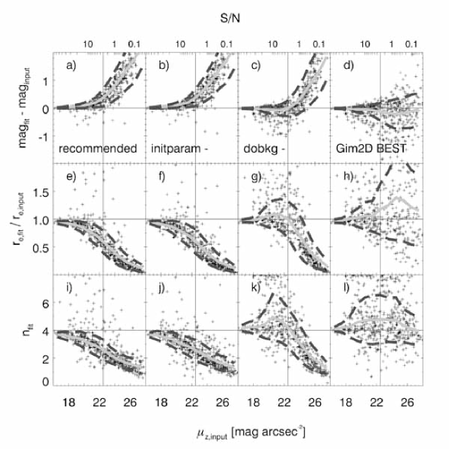
In Figure 6, in the leftmost panels, we show fitting results for
the setup that is recommended on the Gim2d webpage555The GIMFIT2D
description is http://www.hia-iha.nrc-cnrc.gc.ca/STAFF/lsd/gim2d/, and specifies the
last program update of March 19, 2001 (setup K in Table 7).
This recommended setup, in particular, has ‘dobkg’yes and
‘initparams’yes; i.e., Gim2d determines the sky level and fitting
constraints from SExtractor output. As is clear from this plot, this setup produces
unsatisfactory results even for fairly high surface brightness galaxies and where
Gems survey completeness is still quite high. The systematic errors are already
% in near the sky level. Fitting results are strongly systematically
biased towards fainter magnitudes, smaller sizes and lower concentrations.
As most galaxy surveys aim to push their analysis down to faint levels, the ideal
performance of any fitting code is to provide parameter estimates that are free of
significant systematic trends. Therefore, we deem the recommended setup to not be
suitable for the Gems survey. In an attempt to improve the Gim2d performance,
we tried a number of different strategies, among them different settings of
‘initparams’ and ‘dobkg’.
Through extensive testing, we find that the best results are obtained when both ‘initparams’no and ‘dobkg’no (see rightmost panels in
Figure 6), and when the SExtractor local background is used (see
§3.2.3). Setting ‘initparams’no and dobkgyes produces
very modest improvement. Setting ‘dobkg’no and initparamyes helps
considerably, giving satisfactory results for galaxies with surface brightness
higher than the sky surface brightness666This is the setup that was used by
McIntosh et al. (2005) for their study of the evolution of the early-type
galaxy luminosity–size and stellar mass–size relations. Their sample of
galaxies all had F850LP surface brightness brighter than 22.5 mag arcsec-2,
and inspection of the third row of panels in Fig. 6 and setup J
in Table 7 shows that at these limits the Gim2d fitting
results suffer from % biases.. As can be seen in Fig.
6, using a fixed background (dobkg’no) and setting
initparams’no removes the strong systematic trend towards poorer fits for
low surface brightness galaxies, albeit with large scatter at the faint end. As
explained in §3.2.1, the initparams’no option allows
Gim2d to explore the full range of parameter space when determining the best-fit
solution. In contrast, setting this option to ’yes’ narrowly constrains the
magnitude and for objects where the SExtractor segmentation map severely misses
the total extent of galaxies below the sky brightness. It is worth noting that
compared to these two parameter choices, other effects such as the precise fixed sky
value used (see §3.1.2) and the image size
(§3.2.4) appear to produce only minor improvements.
| Parameter | min | max |
|---|---|---|
| mag | 20 | 27 |
| 0.3 | 500 | |
| ellipticity | 0.0 | 1.0 |
| PA | all | all |
| 0.2 | 8.0 | |
| centering x | 0 | 3.0 |
| centering y | 0 | 3.0 |
The minimum and maximum limits of the parameter space that we allowed in our best setup are manually set to span more than the entire range of the simulations in terms of size, luminosity and Sérsic index, more than the physically useful parameter range of real galaxies, so that the solutions are not ‘pinned up’ against the boundary values artificially imposed on them (the actual values are given in Table 6). Fits that ran into any of the given fitting constraints were removed from the sample for the analysis in this paper.
From our findings, we strongly recommend that Gim2d users avoid the dobkg=yes option and be cautious of the surface brightness effects that arise when using initparam=yes.
3.2.3 Gim2d sky test
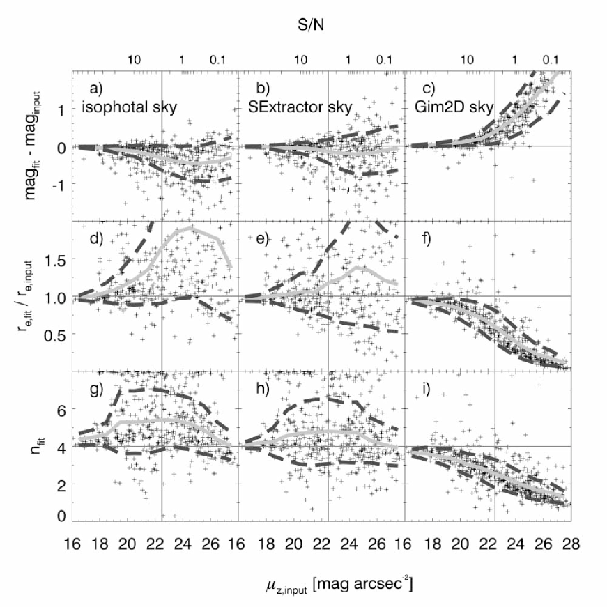
In the above, we showed that sky value estimation can dramatically affect Gim2d fits using the default (recommended) setting. In this section, we repeat the sky
analysis for Gim2d as carried out in §3.1.2 for Galfit. We
tested Gim2d using SExtractor local sky (setups A, B and C in Table
7) and the isophotal sky that we used for Galfit (setups D,
E, F, G and H). We carried out one test – setup I – where we used the ‘real’
background of 18.14 counts, determined on the ‘sky’ image used in the simulation
process. Such a setup is of academic interest only, as for real galaxies it is
impossible to measure such a sky value. Nonetheless, this test gives insight into
the performance of Gim2d when the actual, known, sky value is used as an input
for galaxy fitting. For setup J and K we tried fixing the sky background to the
value determined directly by Gim2d (‘dobkg’=yes). We show results from
these different tests in Figure 7.
It is interesting that Gim2d performs somewhat better using SExtractor local sky, whereas we showed in §3.1.2 that Galfit performs somewhat better using the isophotal sky from Galapagos. It is likely that the cause of this behavior is related to how Galfit and Gim2d deal with nearby neighbors. Since Galfit simultaneously fits neighboring galaxies which overlap with the galaxy of interest, the isophotal sky estimate better represents the background pedestal that is common to the neighboring sources. Gim2d, on the other hand, is unable to simultaneously fit neighbors, and relies on masking neighbors using the SExtractor segmentation map. Thus the ‘effective sky’ for Gim2d includes flux from the outer parts of the galaxy itself and neighboring sources; as the SExtractor sky is derived from the same ‘sky’ area used for fitting, it is a more appropriate value.
3.2.4 Gim2d other tests
| Setup | Sérsic | ratio | ratio | Quality | ||||||||
|---|---|---|---|---|---|---|---|---|---|---|---|---|
| mean | mean | mean | mean | mean | ||||||||
| A | 164/540 | 4.34 | 0.61 | 1.02 | 0.13 | -0.04 | 0.07 | 1.01 | 0.05 | 0.00 | 2.2 | 7.02 |
| B | 168/533 | 4.37 | 0.43 | 1.02 | 0.09 | -0.03 | 0.05 | 1.01 | 0.06 | -0.16 | 1.5 | 8.38 |
| C | 165/549 | 4.32 | 0.56 | 1.01 | 0.10 | -0.03 | 0.07 | 1.02 | 0.06 | -0.10 | 1.8 | 6.31 |
| D | 161/533 | 5.57 | 1.49 | 1.14 | 0.22 | -0.14 | 0.13 | 1.02 | 0.07 | -0.20 | 2.0 | 154.57 |
| E | 164/531 | 4.84 | 0.76 | 1.11 | 0.17 | -0.09 | 0.08 | 1.01 | 0.06 | -0.17 | 2.0 | 44.42 |
| F | 165/539 | 4.75 | 0.67 | 1.10 | 0.17 | -0.08 | 0.08 | 1.01 | 0.06 | 0.05 | 2.0 | 35.63 |
| G | 162/539 | 4.82 | 0.75 | 1.10 | 0.17 | -0.08 | 0.07 | 1.01 | 0.06 | 0.34 | 2.2 | 42.02 |
| H | 161/545 | 4.81 | 0.76 | 1.12 | 0.16 | -0.09 | 0.09 | 1.01 | 0.06 | -0.03 | 1.6 | 40.63 |
| I | 163/533 | 5.68 | 1.40 | 1.27 | 0.30 | -0.16 | 0.14 | 1.01 | 0.06 | -0.03 | 1.7 | 177.28 |
| J | 167/551 | 3.30 | 0.49 | 0.82 | 0.14 | 0.09 | 0.09 | 1.00 | 0.05 | -0.18 | 1.9 | 30.40 |
| K | 168/546 | 3.33 | 0.51 | 0.83 | 0.13 | 0.09 | 0.09 | 1.01 | 0.05 | -0.01 | 1.6 | 28.32 |
Note. — This Table summarizes the results from all Gim2d testing for bright galaxies; see Table 8 for results for faint galaxies.
gives the numbers of galaxies selected from the total sample of that Gim2d returns a result for each setup. The following columns give deviations (resistant mean values clipped at ) from the simulated value and scatter for the 5 key fitting parameters. The values given are values computed iteratively for all galaxies within 3 .
The last column gives the fit quality as defined in Table 4.
Explanation of the setups:
(A) SExtr. local bkg, initparam=no, , image sizes, best setup
(B) SExtr. local bkg, initparam=no, , image sizes
(C) SExtr. local bkg, initparam=yes, , image sizes
(D) isoph. bkg, initparam=no, , image sizes
(E) isoph. bkg, initparam=no, , and image sizes
(F) isoph. bkg, initparam=no, , image sizes
(G) isoph. bkg, initparam=no,, and image sizes
(H) isoph. bkg, initparam=yes, , image sizes
(I) , initparam=no, , image sizes
(J) dobkg=yes, initparam=no, , image sizes
(K) dobkg=yes, initparam=yes, , image sizes, recommended setup
| Setup | Sérsic | ratio | ratio | Quality | ||||||||
|---|---|---|---|---|---|---|---|---|---|---|---|---|
| mean | mean | mean | mean | mean | ||||||||
| A | 151/540 | 4.63 | 1.45 | 1.38 | 0.78 | -0.20 | 0.55 | 1.05 | 0.23 | -1.10 | 7.4 | 24.83 |
| B | 149/533 | 4.52 | 0.92 | 1.44 | 0.67 | -0.23 | 0.43 | 1.05 | 0.21 | -0.13 | 7.0 | 17.35 |
| C | 154/549 | 2.46 | 0.86 | 0.50 | 0.23 | 0.57 | 0.48 | 1.01 | 0.19 | -0.64 | 5.5 | 149.08 |
| D | 147/533 | 5.52 | 1.36 | 3.22 | 1.93 | -0.76 | 0.57 | 1.00 | 0.20 | -1.22 | 10.6 | 148.96 |
| E | 147/531 | 5.05 | 1.27 | 1.89 | 0.95 | -0.47 | 0.49 | 1.02 | 0.16 | -1.17 | 7.6 | 69.38 |
| F | 149/539 | 5.13 | 1.26 | 1.94 | 0.93 | -0.47 | 0.46 | 1.03 | 0.20 | -1.00 | 6.3 | 80.32 |
| G | 148/539 | 5.24 | 1.30 | 2.36 | 1.45 | -0.52 | 0.51 | 1.02 | 0.16 | -1.43 | 6.5 | 97.78 |
| H | 153/545 | 2.45 | 0.92 | 0.53 | 0.27 | 0.53 | 0.50 | 0.96 | 0.16 | -0.88 | 8.1 | 150.72 |
| I | 146/533 | 5.38 | 1.19 | 2.84 | 1.51 | -0.73 | 0.53 | 0.99 | 0.25 | -0.88 | 7.0 | 122.88 |
| J | 155/551 | 1.79 | 0.44 | 0.28 | 0.11 | 1.08 | 0.49 | 1.02 | 0.19 | -0.57 | 9.2 | 306.48 |
| K | 154/546 | 1.78 | 0.40 | 0.28 | 0.12 | 1.10 | 0.47 | 1.04 | 0.15 | -1.86 | 7.5 | 310.23 |
To determine the best-fitting setup to use with Gim2d, we performed 11 different tests (rows A-K) as shown in Tables 7 (bright galaxies) and 8 (faint galaxies). For the ‘bright’ galaxies, we selected all galaxies with magnitudes arcsec-2 and (representing the sample of early-type galaxies from McIntosh et al. (2005), i.e., those important for surveys of early-type galaxy evolution) from the set of galaxies in the sample for which Gim2d returned a result. The ‘faint’ sample included galaxies with magnitudes arcsec-2. We then calculated the mean of the recovered value or ratios of the different fit parameters and the 68% confidence interval.
In our visual examination of the properties of the outliers in these distributions, we found that most of the non-Poisson scatter is caused by contamination of the outer isophotes of the object of interest by nearby neighbors. While this issue is discussed in more detail later in §4.1.3, we illustrate this behavior by running Gim2d on 3 different postage stamp widths of (setup B), (setup A), and (setup D). These tests find that there is an increase in scatter for larger image size, consistent with the expectation of contamination. Using reduces the extreme outlier fraction somewhat from . Yet, since such outliers are a small fraction of the objects, this change in postage stamp size had relatively little impact on the RMS scatter (see tables 7 and 8). The best-fit stamp cutouts we adopt here have sides equal to . This seems to be the best compromise between a postage stamp large enough so that Gim2d includes enough of the important outskirts of the galaxies for fitting, but small enough that neighboring galaxies are reasonably rare and CPU requirements are reasonable. For comparison, the stamp sizes used in Galfit fits are nearly always larger in area than , due to the requirement of simultaneously fitting neighboring galaxies. We will further quantify the effect of neighboring galaxies in §4.1.2 using the set of simulated spheroids examined there.
We also tested whether the initial number of ICF models affected our fitting results. Holding all other setup choices constant we compared the results from fits to the simulations with the default value of (setup F in Table 7), to results for (setup E) and 400 (setup G). We found that the results are independent of the number of ICF models.
3.2.5 Gim2d best-fitting setup
As is apparent especially from Table 8 and Figure 6, the best combination of parameters for our simulations was given by setup A, using SExtractor background (dobkg=no), initparam=no and as image sizes. We choose this setup to be our best and use it throughout this paper to compare Gim2d results with Galfit results.
4. GALFIT/GIM2D Comparison Using Optimized Setups
In this section, we discuss the results of testing our best setups of Gim2d and Galfit. Section 4.1 describes the results obtained using the simulated images with artificial distributions of galaxy parameters as explained in §2. Section 4.2 describes a very similar test using simulated galaxies having more realistic parameter distributions, as derived from real galaxies recovered from individual Gems survey fields. Section 4.3 sums up the results of tests where real images of different depths were fit and the results intercompared.
4.1. Results of Fitting Simulated Galaxy Images
4.1.1 Results of pure disk simulations
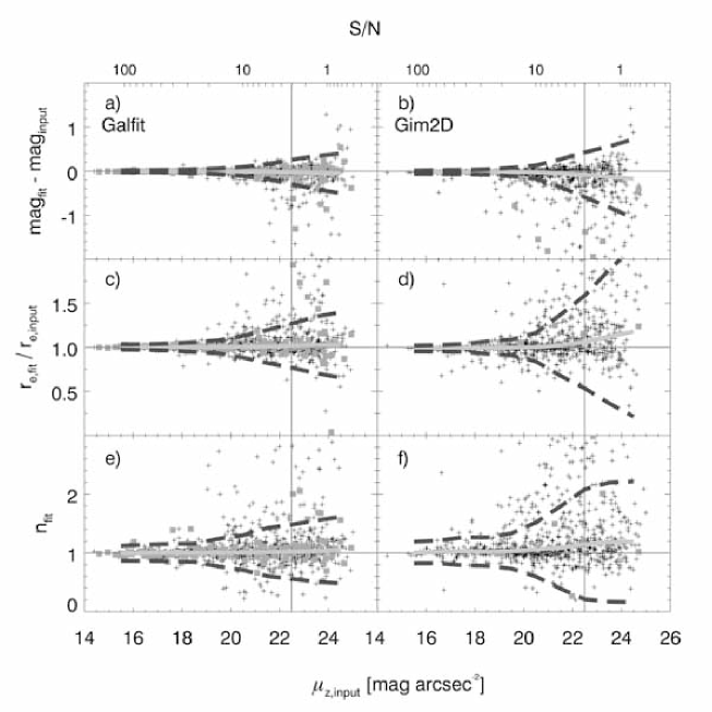
Figure 8 shows both Galfit and Gim2d results for the set of simulated disk galaxies with an exponential light profile. Of the 1600 galaxies simulated in this sample, 997 (62%) were recovered by SExtractor. Of these, 979 (98%) were successfully fitted by Galfit, 12 (1.2%) ran into constraints, 6 (0.6%) fits crashed. Gim2d fitted 870 (87%) successfully, 46 (5%) ran into fitting constraints, 81 (8%) of the fits crashed. There are 4 (0.4%) galaxies for which both codes failed.
Crosses in Figure 8 represent galaxies that were fitted by both codes. Grey squares show galaxies that were fitted by that code only; the other code failed to return a useful result either through running into one of the fitting constraints, or the fit crashed. The thick light-grey line and the thick dashed dark-grey line indicate the mean value and the lines for different surface brightness bins of all galaxies that were fitted using that code. The left column shows fitting results using Galfit, the right column shows the results of the same set of simulations using Gim2d. The X-axis, showing the simulated surface brightness of the galaxies, is the same for all 6 plots. The 3 rows show the results for magnitude (plots a and b), size (c and d) and Sérsic index (e and f), respectively. The thin vertical line indicates the brightness of the sky background within the Gems survey. This is also roughly the limit up to which real galaxies are used for science within Gems. The Y-axes show deviations of the fitting values to the true parameter values, the horizontal thin line indicating the ideal value, which, in case of this galaxy sample, is simply the simulated value.
We will discuss here and in all other sections the behavior of the codes in 3 different surface brightness bins: firstly, the galaxies of highest surface brightness which one clearly would want to be fitted well with any code; secondly, galaxies within a surface brightness bin of 1 magnitude around the surface brightness of the sky; and thirdly, the faintest galaxies, much fainter than the sky surface brightness. The third are the galaxies that are obviously hardest to fit. Here the results from the two codes differ the most from each other.
To summarize our general findings, for =1 galaxies brighter than the sky’s surface brightness, there is no significant mean offset between the input and recovered values in Figure 8; however, the scatter in the Gim2d results is somewhat larger. For this sample of galaxies, this would mean that the final results would be statistically unaffected by one’s choice of fitting code, but for individual objects the reliability of the Galfit results is slightly higher.
For galaxies around the sky surface brightness, there are small systematic trends and increased scatter for our setup of Gim2d: a size ratio of 1.06 (, ) for Gim2d and a ratio of 1.02 for Galfit (). This trend continues towards fainter surface brightness, although at no point does the systematic size offset exceed 20%.
From Figure 8 (grey squares show objects fitted only by the respective code), one can easily see that Galfit returns a result more often than Gim2d, although the fraction of galaxies with failed fits is small in both cases. It is interesting to note that the properties of galaxies with failed fits is somewhat different between the two codes: galaxies not fit by Galfit (those fit only by Gim2d) are fainter than average, the parameters are discrepant even using Gim2d, whereas galaxies not fit by Gim2d (those fit only by Galfit) are fit almost as well by Galfit as other galaxies with the same surface brightness.
4.1.2 Results of pure spheroid simulations
Figure 9 shows the same plots as Figure 8 but for the simulated set of profiles representing the light profile of a typical early-type galaxy. The total number of galaxies recovered in this sample out of 1600 simulated objects was 1091 (68%). Of these, only 2 (0.2%) crashed in Galfit, 56 (5.1%) ran into constraints; Gim2d crashed on 31 galaxies (2.8%), 36 (3.3%) additional fits ran into fitting constraints. 54 (5.0%) galaxies were fitted by Gim2d that were not fitted by Galfit, 63 (5.8%) galaxies were fitted by Galfit and not fitted by Gim2d, both codes crashed on 4 (0.4%) galaxies in common.
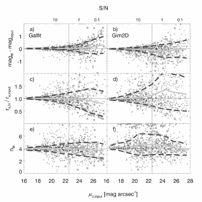
When comparing Figure 9 to Figure 8, one should be aware that the -axis is shifted by 2 magnitudes arcsec-2 towards fainter surface brightness, and that the dashed lines for clarity indicate instead of as in Figure 8. It is clear that both codes recover the parameter values for galaxies significantly less accurately than was the case for the disks, resulting in a substantially larger scatter. This is due to two different effects. Firstly, spheroidal profiles are in principle harder to fit due to the importance of the outskirts of the light profile – this makes using an appropriate sky estimate much more important for a successful fit. Secondly, due to the large amount of light in the faint wings of the galaxies, neighboring objects have a much bigger influence on the fit of the galaxy of interest than was the case for the exponential light profiles. This effect is particularly important for this simulated galaxy sample, because it was designed to have an unrealistically high number of large galaxies.
As was the case for disk galaxies, both codes are basically indistinguishable for high surface brightness galaxies in a statistical sense. For galaxies with surface brightness close to that of the sky, our implementation of Galfit recovers slightly better parameter values than Gim2d (size ratio of 1.00, and a somewhat asymmetric error distribution for Galfit; size ratio of 1.14, and more asymmetric errors for Gim2d). The trend continues towards lower surface brightness, with the Gim2d showing increasingly important systematic offsets and a substantially increased scatter. The directionality and asymmetry of the scatter in all plots (Gim2d and Galfit) are caused by neighboring contamination that is not fully removed, keeping in mind that 32% of the simulated galaxies escape detection by SExtractor because of their low surface brightness.
4.1.3 Deblending effects
Given the significant differences in philosophy when it comes to the deblending techniques between Galfit (multiobject fitting & masking) and Gim2d (masking only), we explore the recovery of input parameters as a function of the immediate environment of a galaxy for both codes. We analyze the subset of 390 (out of a total of 1033) simulated galaxies where Galapagos decided that Galfit needed to simultaneously fit two or more profiles. This has the advantage that only significant neighbors are included in this analysis and should be sufficient to demonstrate the magnitude of the influence of deblending on the quality of galaxy fitting with Galfit and Gim2d.
The results are summarized in Figure 10, showing the difference between recovered and input magnitude as a function of the distance to the next neighbor (left) and as a function of the brightness of this neighbor (right).
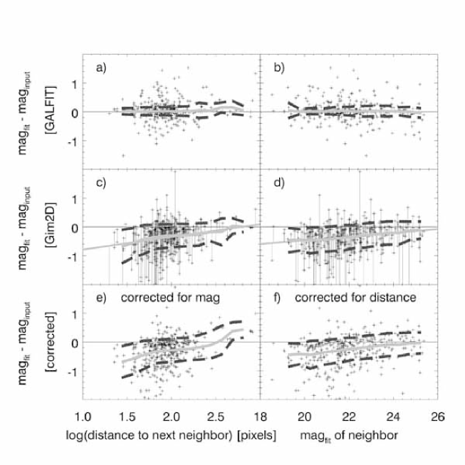
Fitting neighboring objects simultaneously, Galfit (panels a and b) is able to deblend these galaxies reliably, and the deviations of the fitting magnitudes is independent of both distance and brightness of the closest neighbor. For Gim2d (panels c and d), it is clear that fitting residual is a strong function of both distance and brightness of the nearest neighbor. The closer and brighter a neighboring object is, the larger is the magnitude deviation. In an attempt to disentangle the influence of distance and brightness, we try to correct for the systematics observed in panels c and d by removing the offsets and the slope, showing the results in panels e and f. It is clear that distance and brightness effects of nearest neighbor cannot be easily corrected, thus can significantly impact the performance of Gim2d in recovering the true parameters for simulated galaxies. For isolated galaxies, Gim2d does an excellent job of recovering the properties of galaxies.
4.2. Results of Simulations representing simulated GEMS tiles
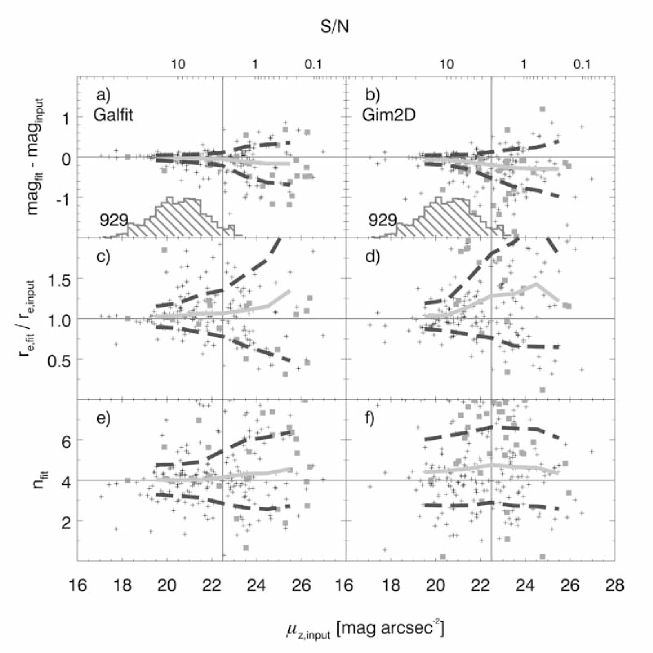
Bearing in mind the importance of neighboring galaxies in determining the quality of fit, we repeated the above analysis using a sample of galaxies where and galaxies were intermixed with realistic clustering, sizes and magnitudes. Towards this goal, simulations were produced from the Galfit results of two real Gems tiles using recovered values of magnitude, position and size. The only parameter that was changed was the Sérsic index. Every galaxy with a real Sérsic index of 2.5 or smaller was simulated with a Sérsic index of 1; all others with a Sérsic index of 4. These simulations have the advantage that they are better able to estimate the uncertainties of galaxy fits with Gems data.
The results are shown in Figures 11 and 12. It is worth noting that the range in galaxy surface brightness is much smaller in these simulations, although we have left the -Axis the same as in the previous plots to facilitate comparison with these. We also show the surface brightness histograms of galaxies used in Barden et al. (2005; disk galaxies) and McIntosh et al. (2005; spheroidal galaxies), to show which areas of parameter space are especially important for scientific analysis of data.
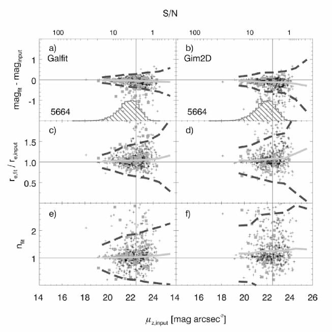
Inspecting Figs. 11 and 12, it becomes clear that Gim2d and Galfit perform more similarly for galaxy populations with clustering and properties typical of medium-depth cosmological HST surveys than for purely simulated data. Galfit shows increased scatter and mild systematic offsets compared to the earlier simulations. In the case of the galaxies the difference in behavior is especially pronounced: it is clear that the presence of realistically clustered galaxies around =1 galaxies is a larger source of random error in galaxy fitting for both Galfit and Gim2d than in pure =1 simulations. Gim2d shows very similar behavior compared to the earlier simulations, with still larger scatter and systematic offsets than Galfit.
4.3. Results of deep-shallow tests using GOODS and GEMS data
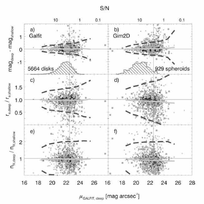
Simulations have the disadvantage that the galaxies have unrealistically simple structure and light-profiles that are known a priori to be the same as the profiles used for fitting. Accordingly, in this section we test the performance of the codes on real galaxies. This goal is not straightforward to achieve, inasmuch as one does not know what the real parameters of a given galaxy are, or indeed whether or not real galaxies are well described by the Sérsic light-profile that was used during our analysis. Instead, we take an empirical approach and test whether the fitting results obtained for real galaxies are sensitive to the image depth by comparing fitting results from the same galaxies in the 1-orbit depth Gems survey and the overlapping 5-orbit depth Goods survey. If they were sensitive to the image depth, it would show that the Sérsic profile is of limited applicability in describing the light profile of real galaxies.
Inspection of Figure 13 shows clearly that both codes are reasonably self-consistent when fitting the same galaxies on images of different depth, i.e. neither Galfit nor Gim2d depends strongly on image depth. While robustness to image depth does not imply that the fitting results are necessarily correct, it does give confidence that issues such as low surface brightness disks missing from shallow HST imaging, departures from Sérsic profiles at fainter surface brightness levels, etc., do not appear to seriously compromise the reliability of fitting parameters in 1-orbit depth HST/ACS data.
4.4. Error estimations from GIM2D and GALFIT
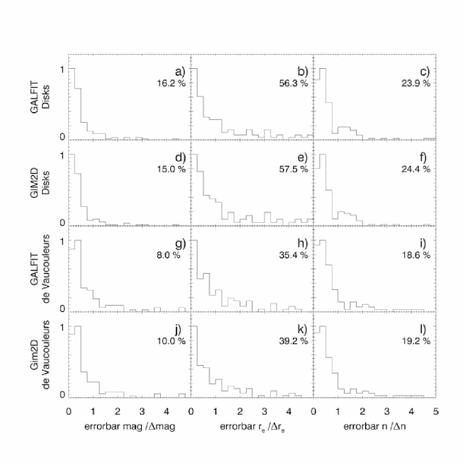
It is interesting to consider if the internal error estimates from Galfit and Gim2d are reasonable reflections of the more realistic uncertainties given by how well the codes recover input parameters for simulated galaxies. In Fig. 14, we address this issue by exploring the distribution of the error estimate divided by the deviation of the fit result from the true value . One can see a strong peak of values with , i.e., for these galaxies the deviation is much larger than the error estimate 777This behavior was the motivation for plotting / instead of the more intuitive quantity /.. Under the assumption that the error estimates are correct, should be 1 for 68% of the galaxies. Fig. 14 shows that for much less than 50% of the cases; i.e., both Galfit and Gim2d substantially underestimate the true fit uncertainties, clearly indicating that the dominant contribution to fitting uncertainty is not shot and read noise; instead contamination by neighbors, structure in the sky, correlated pixels, profile mismatch, etc., dominate the errors. Fig. 14 shows no difference between the histograms of for Galfit and Gim2d; i.e., Galfit and Gim2d both underestimate the errors to a similar extent. Accordingly, in this work and all other Gems works, we have not used the error estimates given by Galfit or Gim2d on an object-by-object basis, relying instead on the mean and width of the parameter distributions from Figs. 11 and 9 at the surface brightness of the galaxy in question.
4.5. Further considerations
In the course of our preparation of Barden et al. (2005) and McIntosh et al. (2005), we found that there were two additional practical considerations that potential users of Galfit and Gim2d may wish to consider.
-
•
Galfit is substantially less CPU intensive than Gim2d, reducing the cost and time of fitting large datasets.
-
•
Gim2d, at least in our implementation, failed to return a fitting result reasonably frequently, requiring manual intervention to restart the code. When trying to fit large datasets, we found this to be labor-intensive. In contrast, Galfit treated each fit as an individual task and therefore was run from shell scripts one fit after the other; if Galfit does not return a fitting result, the script automatically starts the next fit, requiring no interaction from the user.
5. Comparison with Pignatelli et al. (2006)
In this paper we present an extensive and thorough test of the two different 2-D galaxy fitting codes Galfit and Gim2d. In this section, we compare our results with Pignatelli et al. (2006), who compared results from testing these two codes with their own 1-dimensional profile fitter, Gasphot.
Pignatelli et al. conclude that Gasphot performed substantially better for significantly (realistically) blended objects than either Galfit or Gim2d. In the course of our testing, we found a number of differences between our analysis and Pignatelli et al. (2006), which we felt may significantly affect their conclusions.
-
•
For the simulations examined in this paper, they used the IRAF task
mkobject, which, as we described in §2, is inexact for the inner pixels of a simulated galaxy light profile. According to initial tests, the differences in the profiles can lead to systematic errors of up to 10-20% in the fitting parameters using Galfit due to the lack of oversampling of the inner pixels when using at least our settings of artdata parameters, and depending on the exact profile parameters. As we used our own simulation script in IDL, improving the profile from IRAF might be possible by using different parameters settings. -
•
In their paper, Pignatelli et al. allow the sky value to be fitted as a free parameter for all three codes. We argue in this paper that this is a non-optimal way to run any galaxy fitting code: not only would one be subject to errors from irregularities around a Sérsic profile, but also the tests shown in this paper show that fitting the sky level as an additional parameter leads to significantly worse fits (especially in the case of Gim2d). Estimating a value for the sky before running the fitting codes and keeping this value fixed returns more accurate galaxy parameter values.
-
•
Pignatelli et al. state that all automatic tools are likely to have problems with blended objects. Like them, we find that deblending is necessary when setting up fitting routines. Masking out blended objects, while better than doing nothing at all, still leads to significantly biased results: this appears to lie at the root of Gim2d’s difficulties in fitting some simulations (Fig. 10). We find, furthermore, that if one fits multiple galaxies simultaneously (as is recommended when using Galfit), Galfit returns stable unbiased galaxy parameters, even in strongly-blended cases (and in cases with intermixed and galaxies in which galaxies play an important role and which was not tested in the paper by Pignatelli et al. (2006); compare to § 4.2 in this work). Their argument that Galfit does not deal well with blended galaxies is an artefact of the mode in which they chose to use Galfit, in particular the lack of simultaneous fitting of neighboring objects.
-
•
Pignatelli et al. only show the Gim2d results for =4 galaxies; according to our tests these are the hardest galaxies to reliably fit, and showing only those galaxies leads to a false impression of the frequency and severity of Gim2d’s difficulties with nearby neighbors. Also, it seems that Pignatelli et al. (2006) have used the standard setup for Gim2d, which, according to our tests, behaves poorly for faint galaxies: the influence of this decision on their fitting results is unknown.
6. GEMS GALFIT results
In this section, we present the Galfit F850LP-band fitting results of all 41,495 Gems objects that were found by SExtractor. We include fit results for all unique objects, be they stars or galaxies. Some objects appear on two or more Gems frames; in this case the fit results for the images lying furthest from the frame edge was taken. Table 9 shows the 10 first objects in the catalog and gives the format of the catalog published in the online version of this paper. It includes the following values:
-
1.
RA (1), Dec (2): RA and DEC, given by SExtractor(J2000).
-
2.
tile (3): the Gems tile in which the galaxies appears
-
3.
Snum (4): the SExtractor catalog number of this object
-
4.
GemsID (5): the identification of the galaxy within the Gems project.
-
5.
PosX (6), PosY (7): the position [pixels] of the galaxy in this given Gems tile.
-
6.
sky (8): The background pedestal as returned by Galapagos and used during the fit with Galfit.
-
7.
The Galfit results (9-13): magnitude, halflight-radius , Sérsic index , Axis Ratio , and position angle (both with respect to the image, , and with respect to the WCS, defined north-to-east, ) as well as their ‘uncertainties’. These uncertainties are not the errorbars returned by Galfit; as shown in §4.4 these errorbars do not reflect the true uncertainty of the fit. We use a statistical method to derive the error estimates from our simulations. We first estimate from our simulations the scatter of the distribution (of the and galaxy sample, respectively) at the given surface brightness of the real object for and simulations. Then, we perform a linear interpolation between the and to estimate . We do not extrapolate; galaxies with are given the value of the sample, galaxies the value of the sample. We further adopt a minimum uncertainty for each fitting parameter (0.01 mag for mag, 0.01 pixels for , 0.01 for , 0.001 for and 0.1 deg for PA). In the table published online and on the Gems webpage, the uncertainties are stored in extra columns.
-
8.
(14): A flag showing which fits ran into any of the fitting constraints (0: fit ran into constraint, 1: fit did not run into any of the constraints).
-
9.
(15): A flag showing which galaxies would be selected according to the selection criteria given in Barden et al. (2005) (0: object would not be selected for analysis, 1: object would be selected for analysis). The primary effect of the selection is to discard stars and very low surface brightness objects.
As is clear from Fig. 15 and 2, the catalog has strongly varying completeness, primarily as a function of surface brightness. Many applications of the Gems catalogs require a good understanding of these completeness properties. In Barden et al. (2005) and McIntosh et al. (2005), we used the simulations presented in this paper to quantify the effects of completeness. Accordingly, we have made extensive suites of simulation catalogs available to interested users on the Gems webpage to allow detailed examination of systematic errors in fitting and sample completeness. These issues are discussed in substantially more detail in Rix et al. (2004), Barden et al. (2005) and McIntosh et al. (2005).
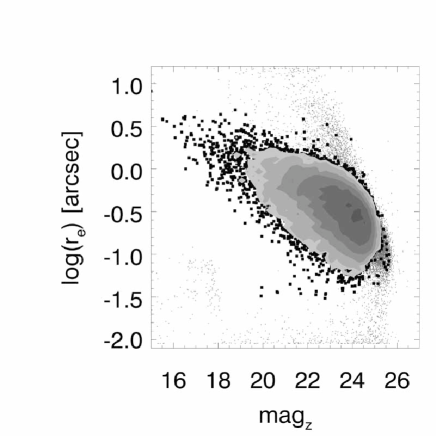
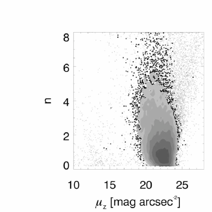
Figure 16 shows the parameter distribution of the subset of 34,638 objects for which the fit did not run into fitting constraints. Galaxies plotted in black and indicated by the contours would pass the selection in Barden et al. (2005) . One can see that galaxies discarded (plotted in grey) are mostly faint, low surface brightness galaxies. Another important class of objects thrown out of the sample are objects with either very small sizes or relatively small sizes at high magnitudes. These are identified as stars (or saturated stars) by the automated selection criteria in Barden et al. (2005). Although all these objects are still included in Table 9, one should be very careful when using their fitting results. All these galaxies are indicated by .
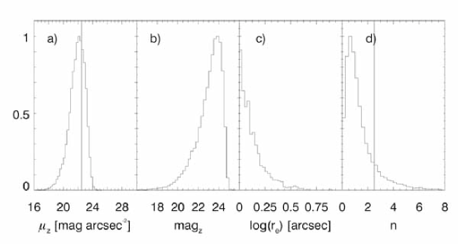
Figure 15 shows histograms of the most important parameters (surface brightness , apparent magnitude, apparent size and Sérsic index ) for the subset of 23,187 objects that would be selected according to the cuts given in Barden et al. (2005).
7. Conclusions
In this paper, we have tuned and tested two parametric galaxy fitting codes – Galfit and Gim2d – for fitting single Sérsic light profiles to both simulated and real data. Our conclusions are the following:
-
•
The performance of both Galfit and Gim2d is a strong function of how the codes are set up; in particular, studies using different setups of parametric fitting codes may arrive at different conclusions about those codes if not properly or optimally used.
-
•
The recommended setup of Gim2d, using
‘dobkg’=‘yes’ and‘initparams=‘yes’ is unable to recover the input parameter values of simulated galaxies that were fainter than the sky surface brightness. We strongly discourage users from using these settings, but to instead fix the background to the value local of each galaxy as given by SExtractor and to input very wide model parameter limits. This is very important if the SExtractor segmentation map does not represent the true extent of a galaxy, as was the case for galaxies below the sky surface brightness when using standard SExtractor configurations. -
•
Both codes are able to fit (at least bright) galaxies reasonably well with relatively little bias (Figure 8). Concentrated galaxies are substantially less straightforward to fit, owing to the large amount of light in the faint outer parts of the galaxies. For bright galaxies, the behavior of Galfit is better than that of Gim2d (Figure 9); however, parameters returned by Gim2d are still not significantly biased. For galaxy populations and clustering typical of medium-depth cosmological HST surveys, there are no large differences between results obtained using Gim2d and Galfit for these bright galaxies. For fainter galaxies, the performance of Galfit is substantially better than that of Gim2d. In the set of realistically mixed simulations (Figure 11 and 12) of and galaxies, representing re-simulated Gems tiles, one can see significantly different behavior of the two codes, especially in the recovery of the Sérsic index. Gim2d results are systematically biased to higher Sérsic indices, which, in automated galaxy classification using the Sérsic index to distinguish early- from late-type galaxies, would lead to systematic misclassification of a subsample of (faint) galaxies.
-
•
The errorbars given by both codes underestimate the true uncertainty of the fit by a large factor. One has to use a different approach to derive more realistic errorbars.
-
•
Our testing demonstrated that how a code treats neighboring galaxies can be of great importance. Gim2d only masks out neighbors, which in the tests we ran could lead to poor fitting results for strongly blended objects. Galfit, in contrast, is able to simultaneously fit many objects, and when used in that mode seems to be relatively robust to contamination by neighbors. For this reason, we caution users interested in strongly clustered galaxies against using Gim2d without extensive prior testing.
-
•
Both Galfit and Gim2d are self-consistent and show no discernable dependence on image depth when comparing fitting results from Gems and Goods data.
-
•
Our tests on deep and shallow data show that real galaxies are indeed reasonably well described by general Sérsic light profiles.
-
•
Galfit works best using an isophotal sky value given by Galapagos. If this is not possible, using Galfit to internally derive a sky value is significantly better than fixing the sky to a local value given by SExtractor.
-
•
On the balance, we would tend to recommend Galfit for single Sérsic profile fitting in medium-depth HST/ACS data, as Galfit results are not only somewhat more reliable in the mean, but also have lower scatter and less sensitivity to contamination by neighbors than Gim2d.
References
- Abraham et al. (1996) Abraham, R. G., Tanvir, N. R., Santiago, B. X., Ellis, R. S., Glazebrook, K., & van den Bergh, S. 1996, MNRAS, 279, L47
- Barden et al. (2005) Barden, M., et al. , 2005, ApJ, 635, 959
- Bell et al. (2004) Bell, E. F., et al. 2004, ApJ, 608, 752
- Bell et al. (2006) Bell, E. F., et al. 2006, ApJ, 640, 241
- Bershady, Jangren & Conselice (2000) Bershady, M.A., Jangren, A., Conselice, C.J., 2000, AJ, 119, 2645
- Bertin & Arnouts (1996) Bertin, E., Arnouts, S., 1996, A&A Supplement series,, 117, 393
- Blanton et al. (2003) Blanton, M. R., et al. 2003, ApJ, 592, 819
- Blanton et al. (2003) Blanton, M. R., et al. 2003, ApJ, 594, 186
- Caldwell et al. (2006) Caldwell, J. A. R., et al. 2006, ApJs, in press (astro-ph/0510782)
- Conselice, Bershady & Jangren (2000) Conselice, C.J., Bershady, M.A., Jangren, A., 2000, ApJ, 529, 886
- Conselice (2003) Conselice, C. J. 2003, ApJS, 147, 1
- de Jong (1996) de Jong, R. S. 1996, A&AS, 118, 557
- deVaucouleurs (1948) de Vaucouleurs, G., 1948, Ann. d’Astrophys., 11, 247
- Freeman (1970) Freeman ,K. C. 1970, ApJ, 160, 811
- Giavalisco et al. (2004) Giavalisco, M., et al. 2004, ApJ, 600, L93
- Graham et al. (2005) Graham, A. W., Driver, S. P., Petrosian, V., Conselice, C. J., Bershady, M. A., Crawford, S. M., & Goto T. 2005, AJ, 130, 1535
- (17) Gray, M., and the Stages team, in prep
- Hogg et al. (2004) Hogg, D. W., et al. 2004, ApJ, 601, L29
- Jahnke et al. (2004) Jahnke, K., et al. 2004, ApJ, 614, 568
- Lilly (1998) Lilly, S., et al. 1998, ApJ, 500, 75
- Lotz et al. (2006) Lotz, J. M., Madau, P., Giavalisco, M., Primack, J., & Ferguson, H. C. 2006, ApJ, 636, 592
- McIntosh et al. (2005) McIntosh, D. H., et al. 2005, ApJ, 632, 191
- Peng et al. (2002) Peng, C.Y., Ho, L.C., Impey, C.D., Rix, H.-W., 2002, ApJ, 124, 266-293
- Petrosian (1976) Petrosian, V. 1976, ApJ, 209, L1
- Pizagno et al. (2005) Pizagno, J., et al. 2005, ApJ, 633, 844
- Press (1997) Press, W. H., Teukolsky, S. A., Vetterling, W. T., & Flannery, B. P. 1997, Numerical Recipes in C (Cambridge: Cambridge Univ. Press)
- Pignatelli et al. (2006) Pignatelli, E., Fasano, G., & Cassata, P. 2006, A&A, 446, 373
- Ravindranath et al. (2004) Ravindranath, S., et al. 2004, ApJ, 604, L9
- Rix et al. (2004) Rix, H., Barden, M., Beckwith, S.V.W., Bell, E.F., Caldwell, J.A.R., H ußler, B., Jahnke, K., Jogee, S., McIntosh, D.H., Meisenheimer, K., Peng, C.Y., Sanchez, S.F., Somerville, R.S., Wisotzki, L., Wolf, C., 2004, ApJS, 152, 163
- Ryden (2006) Ryden, B. S. 2006, ApJ, 641, 773
- Sargent et al. (2006) Sargent, M. T., et al. 2006, ArXiv Astrophysics e-prints, arXiv:astro-ph/0609042
- Schade et al. (1997) Schade, D., Barrientos, L. F., & Lopez-Cruz, O. 1997, ApJ, 477, L17
- Schade et al. (1999) Schade, D., et al. 1999, ApJ, 525, 31
- (34) Scoville, N., Aussel ,H., Brusa, M.,Capak P., M. Carollo, C., Elvis, M., Giavalisco, M., Guzzo, L., Hasinger, G., Impey, C., Kneib, J.-P., LeFevre, O., Lilly, S. J., Mobasher, B., Renzini, A., Rich, R. M., Sanders, D. B., Schinnerer, E., Schminovich, D., Shopbell, P., Taniguchi, Y., Tyson, N. D., submitted to ApJ, astro-ph/0612305
- Sérsic (1968) Sérsic, J.L., 1968, Atlas de Galaxias Australes (C rdoba: Obs. Astron., Univ. Nac. C rdoba)
- Shen et al. (2003) Shen, S., Mo, H. J., White, S. D. M., Blanton, M. R., Kauffmann, G., Voges, W., Brinkmann ,J., & Csabai, I. 2003, MNRAS, 343, 978
- Simard (1998) Simard, L., 1998, Astronomical Data Analysis Software and Systems VII, 145, 108
- Simard & Pritchet (1998) Simard, L., & Pritchet, C. J. 1998, ApJ, 505, 96
- Simard (2002) Simard, L., 2002, ApJS, 142, 1
- Trujillo et al. (2001) Trujillo, I., Graham, A. W., & Caon, N. 2001, MNRAS, 326, 869
- Trujillo et al. (2004) Trujillo, I., et al. 2004, ApJ, 604, 521
- Trujillo & Pohlen (2005) Trujillo, I., & Pohlen, M. 2005, ApJ, 630, L17
- Trujillo et al. (2006) Trujillo, I., et al. 2006, ApJ, in press (astro-ph/0504225)
- Wolf et al. (2003) Wolf, C., Meisenheimer, K., Rix, H.-W., Borch, A., Dye, S., & Kleinheinrich, M. 2003, A&A, 401, 73
| RA | DEC | tile | Snum | Gems ID | PosX | PosY | sky | Galfit fitting results | ||||||
|---|---|---|---|---|---|---|---|---|---|---|---|---|---|---|
| mag | image/WCS | |||||||||||||
| [deg] | [deg] | [pix] | [pix] | [cnt] | [mag] | [pix] | [deg] | |||||||
| (1) | (2) | (3) | (4) | (5) | (6) | (7) | (8) | (9) | (10) | (11) | (12) | (13) | (14) | (15) |
| 53.316325 | -28.059058 | s9z01A | 1 | GEMSJ033315.92-280332.6 | 5752.64 | 721.57 | 18.120 | 13.910.01 | 0.320.01 | 6.630.01 | 0.7770.011 | 3.8( 1.6)0.1 | 1 | 0 |
| 53.334888 | -28.062040 | s9z01A | 2 | GEMSJ033320.37-280343.3 | 3786.09 | 368.55 | 18.120 | 15.570.01 | 0.300.02 | 3.390.01 | 0.9380.001 | 84.0( 81.8)0.1 | 0 | 0 |
| 53.340850 | -28.062310 | s9z01A | 5 | GEMSJ033321.80-280344.3 | 3154.69 | 337.72 | 18.056 | 21.580.09 | 13.930.11 | 0.370.26 | 0.7450.056 | 21.4( 19.2)4.4 | 1 | 1 |
| 53.366943 | -28.062952 | s9z01A | 6 | GEMSJ033328.07-280346.6 | 391.45 | 266.85 | 18.355 | 24.140.10 | 5.210.12 | 0.970.27 | 0.7190.059 | -47.8(-50.0)4.6 | 1 | 1 |
| 53.340514 | -28.061939 | s9z01A | 9 | GEMSJ033321.72-280343.0 | 3190.41 | 382.16 | 18.149 | 21.130.32 | 67.080.35 | 5.361.02 | 0.5580.054 | -60.0(-62.2)5.8 | 1 | 0 |
| 53.370589 | -28.062339 | s9z01A | 10 | GEMSJ033328.94-280344.4 | 5.61 | 341.22 | 18.426 | 23.220.12 | 19.790.14 | 0.660.29 | 0.3020.064 | -77.1(-79.3)5.1 | 1 | 0 |
| 53.342879 | -28.061422 | s9z01A | 11 | GEMSJ033322.29-280341.1 | 2940.04 | 444.77 | 18.098 | 23.050.11 | 14.030.13 | 1.000.28 | 0.6190.063 | -38.8(-41.1)5.1 | 1 | 1 |
| 53.342659 | -28.060898 | s9z01A | 12 | GEMSJ033322.24-280339.2 | 2963.58 | 507.56 | 18.171 | 20.050.01 | 0.300.17 | 1.170.92 | 0.1400.001 | 52.4( 50.1)0.4 | 1 | 0 |
| 53.347315 | -28.061235 | s9z01A | 13 | GEMSJ033323.36-280340.4 | 2470.43 | 468.25 | 18.223 | 22.960.08 | 6.300.10 | 1.180.27 | 0.8040.051 | 57.5( 55.2)4.1 | 1 | 1 |
| 53.341322 | -28.059825 | s9z01A | 14 | GEMSJ033321.92-280335.4 | 3105.38 | 636.05 | 18.144 | 21.560.10 | 43.400.12 | 0.450.27 | 0.1230.059 | 50.7( 48.4)4.7 | 1 | 1 |
Note. — This table shows the first 10 objects of the Gems fitting results published in the online version of this paper. For every object that was found by SExtractor we give RA, DEC, the Gems tile name, the SExtractor number of that object, the GemsID (containing RA and DEC) as well as the X and Y position on the Gems tile, so that identification of objects is easily possible. Furthermore we give the isophotal sky value that was used during the fit and the fitting results of the 5 key parameters mag (in apparent F850LP-band magnitudes), (in pixels of 0.03”), Sérsic index , axis ratio and position angle PA in respect to the image (counted counterclockwise from vertical line according to the convention within Galfit) and the world coordinate system (in brackets, north through east). Uncertainty estimates are derived from the simulations, following §4.4. The last two columns show two different flags showing which fits ran into fitting constraints () and which ones would make it into the final galaxy sample used for science according to the selection criteria given in Barden et al. (2005) ().
The complete version of this table is in the electronic edition of the Journal. The printed edition contains only a sample.