Inverse Monte-Carlo determination of effective lattice models for SU(3) Yang-Mills theory at finite temperature
Abstract
This paper concludes our efforts in describing -Yang-Mills theories at different couplings/temperatures in terms of effective Polyakov-loop models. The associated effective couplings are determined through an inverse Monte Carlo procedure based on novel Schwinger-Dyson equations that employ the symmetries of the Haar measure. Due to the first-order nature of the phase transition we encounter a fine-tuning problem in reproducing the correct behavior of the Polyakov-loop from the effective models. The problem remains under control as long as the number of effective couplings is sufficiently small.
pacs:
11.15.Ha, 11.15.Me, 11.10.Wx, 12.40.EeI Introduction
Since the pioneering papers of Polyakov Polyakov (1978) and Susskind Susskind (1979) the confinement-deconfinement phase transition in finite temperature Yang-Mills theory has become a thoroughly studied phenomenon. This is particularly true for the ‘standard’ groups and , but more ‘exotic’ groups like have recently come into focus as well, see e.g. Holland et al. (2003); Greensite et al. (2007). Due to the nonperturbative nature of the problem progress has mainly been achieved via brute force lattice computations.
Nevertheless, it would be helpful to have a simpler and more intuitive understanding of the physics involved. The principal tool for this purpose is the construction and subsequent analysis of effective models. Such attempts also have quite some history going back to the works of Svetitsky and Yaffe Yaffe and Svetitsky (1982); Svetitsky and Yaffe (1982) as well as Polonyi and Szlachanyi Polonyi and Szlachanyi (1982). The basic idea (in the spirit of Landau and Ginzburg) is to use the order parameter of the transition, the Polyakov loop, as a collective degree of freedom and formulate effective theories in terms of it. For gauge groups the rationale behind that is the Svetitsky-Yaffe conjecture Yaffe and Svetitsky (1982); Svetitsky and Yaffe (1982) which states that the Yang-Mills finite-temperature transition in dimension is described by an effective spin model in dimensions with short-range interactions111The reasoning involved strongly relies on center symmetry. The study of more exotic Lie groups (which may not even have a nontrivial center) suggests that the size of the gauge group is also important Holland et al. (2004).. These ideas have initially been taken up in terms of strong coupling expansions Polonyi and Szlachanyi (1982); Green and Karsch (1984); Ogilvie (1984) yielding Ising type spin models with an effective coupling where denotes the Yang-Mills-Wilson coupling. A review of early work in this context may be found in Svetitsky (1986). For an overview of more recent developments we refer the reader to Holland and Wiese (2000).
Early on, it has also been attempted to obtain these effective models, that is their couplings (being the ‘weights’ of the included operators) nonperturbatively via lattice methods. In Creutz et al. (1984); Gocksch and Ogilvie (1985) Creutz’s microcanonical demon method Creutz (1983) has been employed for . An alternative method based on Schwinger-Dyson equations (SDEs) and dubbed “inverse Monte Carlo” (IMC) was developed soon after Falcioni et al. (1986); Gonzalez-Arroyo and Okawa (1987a) and applied to both Deckert et al. (1987); Gonzalez-Arroyo and Okawa (1987b) and Fukugita et al. (1989); Moore and Ogilvie (1990). Since then the IMC approach to lattice gauge theories has largely been dormant with only a few exceptions Hasenbusch et al. (1994); Svetitsky and Weiss (1997).
Inspired by the success of Polyakov loop models Pisarski (2000, 2002); Dumitru et al. (2004) we have recently reinvestigated the feasibility of IMC for the confinement-deconfinement phase transition in a series of papers. Our numerical approach has consistently been complemented by analytical attempts such as strong coupling expansions and mean-field approximations. For the second-order transition our results may be found in Dittmann et al. (2004) and Heinzl et al. (2005). By including up to 14 operators and 3 different group representations we were able to reproduce suitable Yang-Mills observables to a reasonable accuracy. The same is true for the analytically known asymptotic behavior of the effective couplings as a function of . In Wozar et al. (2006) we have started to investigate effective models for which are generalisations of the 3-states Potts model. The critical behavior of these is an interesting subject in its own right. We have found a very rich phase structure with first and second order transitions between symmetric, ferromagnetic and anti-ferromagnetic phases. In addition there seems to be a tricritical point rendering mean-field theory approximately exact in its vicinity Wozar et al. (2006); Wipf et al. (2007)
In relating the effective models to Yang-Mills via IMC one expects to encounter new difficulties. The first technical problem to overcome is to find the SDEs which are less straightforward than for as the group manifold no longer is a sphere. This problem has been solved in Wozar (2006) and Uhlmann et al. (2007). As the phase transition is of (weak) first order, hence not continuous, the determination of the effective couplings might require fine-tuning raising the question of stability of the solutions. This will be one of the main issues to be addressed in what follows.
The remainder of the paper is organized as follows. In Section II we suggest different effective actions as candidates for describing the Polyakov loop dynamics of Yang-Mills theory. In Section III we explain how to obtain the effective couplings via two alternative sets of SDEs and subsequent IMC. Our numerical results are presented in Section IV. Section V concludes our discussion with a summary and outlook. Some technicalities are deferred to Appendices A–C.
II Effective actions
We begin by recalling the lattice definition of the untraced Polyakov loop in the group representation ,
| (1) |
where is the temporal link at time slice and position in representation . Any irreducible representation of is labeled by two integers, , which, in flavor language, count the number of quarks and antiquarks needed to construct the multiplet associated with . The basic building blocks of our effective actions are the group characters associated with the representation , that is the traces of the Polyakov loop (1),
| (2) |
Note that these only depend on the traced Polyakov loop in the fundamental representation, . The trivial character is of course while the first nontrivial ones correspond to the (anti-)fundamental representations and yield just the standard traced Polyakov loop (and its complex conjugate),
| (3) |
Under a center transformation, the characters transform as
| (4) |
Center symmetry is then sufficient to determine the operator content of the effective action if we restrict to nearest-neighbor (NN) interactions. In terms of group characters one finds the general form
| (5) |
where the sum over representations is constrained by center symmetry. Expressing the characters explicitly in terms of the Polyakov loop one easily recognizes (5) as the action suggested by Dumitru et al. Dumitru et al. (2004). Their ‘potential terms’, built from single center symmetric characters located at single sites appear whenever the second adjacent character is trivial, . In this case the typical hopping terms connecting NN sites ‘degenerate’ into ultra-local terms, the one of lowest dimension being the ‘octet loop’ contribution, as indeed . One expects that the couplings decrease with increasing representation labels, , , and , hence that representations of low dimension,
| (6) |
dominate the effective action. To simplify our notation we will henceforth write the action (5) (and generalizations thereof) as a series of the form
| (7) |
where up to 16 different terms will be taken into consideration, albeit not necessarily within one and the same ansatz. A list of the operators may be found in Appendix A where we allow for next-to-NN (NNN) couplings in addition. It is easy to check that each of the terms given satisfies the selection rules for the representation labels necessary for center symmetry.
It turns out (in hindsight) that the ansätze (5) or (7) contain more freedom of choice than actually required which makes the inverse Monte Carlo routines less efficient (see below). To further constrain this freedom we generalise to the strong-coupling approach introduced by Billo et al. Billo et al. (1996) which we already have successfully applied to Heinzl et al. (2005). The basic building blocks are then given by the center symmetric operators connecting NN sites,
| (8) |
The strong coupling expansion then replaces the ansatz (5) by the following somewhat more complicated expression Wozar (2006),
| (9) |
where counts the number of link operators (8) contributing at each order. The coefficients are the couplings between the operators from (8) sitting at NN links in representation . The effective action defined in (9) hence describes a network of link operators of the type (8) that are collected into (possibly disconnected) ‘polymers’ contributing with ‘weight’ . Again, one expects the ‘weights’ or couplings to decrease as the dimensions of the representations and the inter-link distances involved increase. In a strong coupling (small-) expansion truncated at one has and the additional restriction with for a given representation .
To lowest order one finds the universal effective action Polonyi and Szlachanyi (1982)
| (10) |
which is just a single hopping term connecting Polyakov loops at NN sites. This is reminiscent of a generalised Ising model or, more appropriately, a three-state Potts model Potts (1952). As mentioned before the study of these models is interesting in its own right Wozar et al. (2006) but will not be the topic of the present paper which focuses on the relation between the effective actions and Yang-Mills theory.
Again, the most general representation (9) is not too illuminating and we will therefore adopt the notation
| (11) |
A list of the leading NN and NNN action terms can be found in Appendix B.
In principle, without any truncations, the effective actions (7) and (11) have to coincide although the operator bases used are different. Accordingly, there is a linear relationship between the couplings and . However, as the ordering principles for the two ansätze are not the same the relation between the couplings after truncation is not one-to-one but rather of the form
| (12) |
Typically, for a given truncation of the -action (7) the range of the index is larger than that of , i.e. there are more ’s than ’s. Accordingly, the matrices are rectangular with and integer entries. For this reason it is calculationally often more efficient to work with the -action (11) and reobtain the via (12). Our standard choices for the numerical matrices corresponding to different truncations of the effective actions may be found in Appendix C. As the operators appearing in (7) are more intuitive and resemble generalised spin terms we have decided, for the sake of brevity, to present results only for the ’s in this paper.
III Schwinger-Dyson equations and inverse Monte-Carlo
In this section we shortly recapitulate the Schwinger-Dyson equations (SDEs) that have recently been derived in Wozar (2006) and Uhlmann et al. (2007). They will be the main tool to relate the effective actions (7) and (11) to Yang-Mills theory. Our numerical approach benefits from the fact that there are two independent versions of SDEs which in the end, however, should yield equivalent results. The first type of equations is based on an integral identity which is more algebraic in nature than the second type which follows from geometrical considerations.
III.1 Algebraic SDEs
It is useful to parameterize the diagonalized, untraced Polyakov loop by means of two angular variables, and ,
| (13) |
with values in a fundamental region given by the restrictions
| (14) |
As a result, the reduced Haar measure acquires the form
| (15) |
with a nontrivial Jacobian that may either be expressed in terms of characters,
| (16) |
or in terms of the trace of (13),
| (17) |
Using the latter variable leads to the remarkable algebraic identity
| (18) |
such that one can trade for its square root . It is a fact of life that any function vanishing on the boundary of a region satisfies the integral identity
| (19) |
which is reminiscent of integration by parts on the real line, (for functions vanishing at infinity). For our purposes we make the particular choice
| (20) |
with arbitrary and integrate over the domain of given implicitly via (14). This is consistent with the general identity (19) as the reduced Haar measure vanishes at the boundary of the fundamental region (14). Hence, (19) specializes to
| (21) |
where we have used the reduced Haar measure from (18) and reinstated the dependence on the lattice site chosen to be . The derivative of can actually be worked out with the result
| (22) |
To actually obtain genuine SDEs we have to introduce the usual Boltzmann factor . This is done by choosing a special function , namely
| (23) |
with another function required to be invariant,
| (24) |
Plugging in the ansatz (7) for the -action the -derivative of (23) needed for (21) becomes
| (25) |
where the commas denote differentiation with respect to the subsequent argument. Functional integration of (21) with the measure finally yields the desired SDEs,
| (26) |
which comprise a linear system for the effective couplings , generalising analogous results for Dittmann et al. (2004); Heinzl et al. (2005). The experience gained there prompts us to choose the function from the operators in the ansatz for the -action (7). Any index then yields an independent equation. In addition, this choice automatically satisfies the criterion (24) of invariance.
On top of that we will vary the sites and , in particular the distance between them. On a lattice with spatial extent this implies a range of distances where denotes the largest integer . For different operators we thus obtain independent equations for each distance .
III.2 Geometrical SDEs
For any function on a Lie group we define its left derivative in the direction of the generator via
| (27) |
Left invariance of the Haar measure implies a symmetry relation somewhat analogous to (19),
| (28) |
which will serve as a master identity generating all SDEs. As in the previous subsection we would like to integrate over the reduced Haar measure only. Thus, we want the integrand to be a class function. If is such a class function it only depends on the fundamental group characters, , where denotes a fundamental representation of the group element , i.e. or for . For the particular choice , with an arbitrary class function and a fundamental character, the integrand in (28) indeed becomes a class function so that we end up with the ‘reduced’ integral
| (29) |
For we obviously choose the fundamental character as the trace of the Polyakov loop in the fundamental representation, and , slightly different from (23). The left derivatives are worked out as follows Wozar (2006); Uhlmann et al. (2007),
| (30) |
and only depend on the traced Polyakov loop as they should. Finally, to obtain feasible equations we choose among the -derivatives of the , implying the following set of geometrical SDEs,
| (31) |
where, again, the dependence on the lattice site has been made explicit.
III.3 Normalisation
We have seen that, for every pair of lattice sites and , we end up with a linear system of equations for the couplings of the effective theory. Since on the lattice we have both translational and (discrete) rotational symmetry it is sufficient to consider different distances only. These serve as a label for our sets of equations which in a condensed matrix notation may be written as
| (32) |
If we assume a total of unknown couplings collected into the vector we have, by construction of the SDEs, an matrix and an inhomogeneity , hence an independent system of equations, for each distance . The off-diagonal entries of and the vector are typically complex but the couplings have to be real. We therefore distinguish between real and imaginary parts of (32) for different and group them together into the equations
| (33) |
This constitutes an overdetermined linear system of equations for the unknown couplings . In principle, this can be solved by standard least-square methods.
However, this procedure is hampered by a few technical pitfalls. Since the order parameter for the confinement-deconfinement transition is driven by the long-range behavior of the lattice system we have to take into account the fact that equations associated with different distances enter (33) with different multiplicities. On a three-dimensional lattice this entails that an equation for distance has multiplicity
| (34) |
while equations for only appear once. To account for this mismatch we reweight the coefficients of and (for ) with a factor .
Another problem are the large condition numbers of the matrices. To cope with this we employ a simple form of normalization based on the diagonal elements of the matrix . For the algebraic SDEs the diagonal entries of dominate the linear system. For this reason we construct a new diagonal matrix from the according to
| (35) |
By means of a similarity transformation with the real parts of the may be transformed to unity. As a result (33) becomes
| (36) |
Typically, this new system of equations is better conditioned which increases the stability of the results.
IV Numerical results
The IMC method basically amounts to solving the SDEs (26) or (31), the crux being the evaluation of the expectation values in the microscopic ensemble. In our case this is given by a sufficient number of Yang-Mills configurations generated by standard MC routines Cabibbo and Marinari (1982); Creutz (1980); Kennedy and Pendleton (1985). In what follows we will consider three ansätze, one with five NN couplings and two more general ones which either contain NN terms in higher representations or additional NNN couplings. In a strong coupling expansion (which is rationale for the -actions) both the five leading NN terms as well as the NNN ones would be of order while the extended NN ones would be .
IV.1 NN couplings
Before one determines the effective couplings corresponding to Yang-Mills it is prudent to check if the SDEs (26) and (31) derived above are consistent within the effective theories themselves. To test for that we have first simulated an effective theory with five fixed input couplings and tried to reproduce them via IMC. In Table 1 we have listed the outcome of this testing procedure. One notes that the couplings determined via IMC coincide with the chosen input couplings to an accuracy of about 2%, both for the algebraic and geometrical SDEs. This tells us two things, first that our SDEs (26) and (31) are both correct and, second, that IMC works extremely well for the effective theories.
| algebraic | geometrical | |||
|---|---|---|---|---|
Having thus gained confidence in the validity of our IMC approach and its implementation we can move on to apply it to our objective namely to determine effective actions reproducing Yang-Mills thermodynamics, in particular the deconfinement phase transition. The first question we want to consider is whether the effective couplings viewed as functions of the Wilson coupling are sensitive to the phase transition.
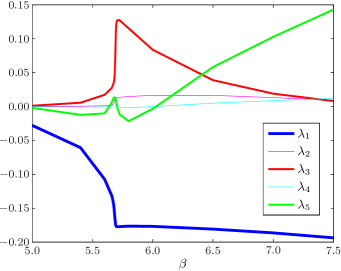
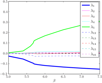
The answer turns out to be affirmative: Fig. 1 clearly shows a rather drastic change in the behavior of the couplings at a value of for all , . Across the transition, i.e. in both phases the dominant coupling is the ‘fundamental’ one, , followed by the octet couplings and . The latter is actually a ‘potential’ coupling in the sense of Dumitru et al. (2004) as it multiplies the center symmetric single-site octet character (see App. A). The couplings and are clearly subdominant.
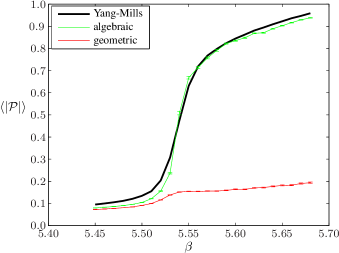
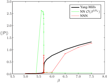
The natural observable to address is, of course, the Polyakov loop which serves as the order parameter of the first-order phase transition. In Fig. 2 we compare the effective and Yang-Mills Polyakov loops for a relatively small lattice of size where the would-be discontinuities (in infinite volume) of the transition are still fairly smooth. Somewhat surprisingly it is only the algebraic SDEs which reproduce the behaviour of the Yang-Mills Polyakov loop reasonably well. The geometrical SDEs, on the other hand, fail to do so, at least in the region just above the transition point. This is a first hint that there is some inherent instability in the IMC procedure – in particular if the geometrical SDEs are used.
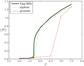
If we move on to larger lattices where the jump of the order parameter at the critical coupling becomes more pronounced one finds the behavior displayed in Fig. 3. Again, the algebraic SDEs work satisfactorily unlike the geometric ones for which, in particular, the sudden rise of the order parameter appears at a larger value of , namely . This is substantially larger than the critical coupling, . Our explanation for this behavior is the fact that, due to the first-order nature of the transition, there are rather sharp phase boundaries in the space of coupling constants, . Hence, a tiny change in the couplings (presumably well within the IMC error bars) may easily have a large effect: by straying into the ‘wrong’ phase the Polyakov loop will suddenly explode or collapse. This nonlinear effect is rather difficult to evade considering the unavoidable (if small) instabilities of the IMC procedure. As a result, as we inevitably increase these inaccuracies by adding more coupling we expect this fine-tuning problem to become enhanced even further. The following subsection will precisely address this topic.
IV.2 NN and NNN couplings
There are (at least) two possibilities to generalise the NN -action of the previous subsection. One may either extend the NN terms to higher group representations or include interactions of larger range, say NNN.
| extended NN | NN + NNN | |||
|---|---|---|---|---|
The new NN terms we will add are of strong-coupling order , the additional NNN terms of order . As we are working at large one cannot predict which ones are going to be more important. Rather, this will be one of the questions to be considered in what follows.
As before we have first tested the consistency of our SDEs. Table 2 shows once again that even for a total of the order of ten couplings the method works well: IMC output reproduces input for the effective theory. The empty input entries in Table 2 correspond to vanishing couplings. For a few sample couplings we have checked that vanishing input correctly entails vanishing output as well.
To determine the behavior of the effective couplings , , as a function of the Wilson coupling we have used a set of configurations per on a -lattice. This amounts to () uncorrelated configurations far away from (close to) the phase transition. The IMC results are shown in Figs. 4 and 5 displaying the effective couplings as functions of . Again we note that the fundamental and octet potential couplings ( and ) dominate in size. More important from a principal point of view, however, is the observation that the behavior of coupling constants is very sensitive to the choice of operators. Let us compare, for instance, the coupling in the two Figs. 4 and 5. For the extended NN ansatz (Fig. 4) it is comparable in magnitude with and and behaves similarly as for the simple NN ansatz of Fig. 1. However, as soon as we include NNN operators its magnitude drops by 100% and its behavior changes drastically (Fig. 5). The latter is also true quite significantly for the octet coupling . This clearly signals an instability of the IMC methods, at least as far as the determination of the couplings is concerned.
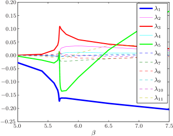
Nevertheless, it might still be possible that largely different sets of couplings lead to more or less identical behavior of observables. Comparing the behavior of the Polyakov loop in the effective and Yang-Mills theories rules out this possibility. As Fig. 6 shows the Polyakov loop when calculated in the effective models is extremely sensitive to the choice of operators and the value of around . For both choices of SDEs the effective order parameter significantly overshoots the Yang-Mills one in a small -range near (see the spikes in Fig. 6). This means that in the space of effective couplings the phase boundary to the deconfined phase have slightly (and for a short range of values) been crossed albeit with drastic effect due to the discontinuous behavior of the Polyakov loop. We conclude that the fine tuning problem encountered in the previous subsection indeed becomes more severe if we include more operators (and hence increase the instabilities of the IMC procedure). For the given number of effective couplings (of order ten) we have not been able to get this problem under control.
V Summary and Outlook
In this paper we have applied the IMC method to study the finite temperature phase transition of Yang-Mills theory. A crucial input were novel Schwinger-Dyson equations based on algebraic and geometrical properties of the Haar measure. The resulting equations constitute overdetermined linear systems for the effective couplings which were solved numerically via least square techniques. The method works well if the number of couplings is sufficiently small, say of the order of five. However, already in this case one notes a fine-tuning problem as the behavior of the Polyakov loop depends in a very sensitive and nonlinear way on the effective couplings. This fact can be traced back to the discontinuities associated with the first-order character of the phase transition. Hence, the problem becomes more pronounced in larger volumes.
If we increase the number of effective couplings and thus, inevitably, the instabilities in their IMC determination, the fine-tuning problem again becomes more severe. This holds to such an extent that we could no longer gain numerical control and hence could no longer reproduce the Yang-Mills behavior of the Polyakov loop in the vicinity of the critical Wilson coupling, . We believe that an improvement on this situation will require nontrivial modifications of the IMC procedure like e.g. smoothening of the loop in order to avoid the unphysical spikes of Fig. 6. In addition, it would be interesting to check whether Creutz’s microcanonical demon method Creutz (1983) mentioned in the introduction yields better results.
We conclude, nevertheless, with the positive statement that the IMC method does work for the first-order transition as well if we allow for only a small number of terms in the effective Polyakov loop actions.
Acknowledgements.
TK and CW gratefully acknowledge their scholarships by the Konrad-Adenauer-Stiftung e.V. and the Studienstiftung des deutschen Volkes, respectively. TH thanks his colleagues of the Plymouth Particle Theory Group for their support.Appendix A Operators for the -actions
In this paper we have used up to 16 different operators appearing in the -action (7):
| (37) | ||||
| (38) | ||||
| (39) |
| (40) | ||||
| (41) | ||||
| (42) | ||||
| (43) | ||||
| (44) | ||||
| (45) | ||||
| (46) | ||||
| (47) | ||||
| (48) | ||||
| (49) | ||||
| (50) | ||||
| (51) | ||||
| (52) |
The NN and NNN relationships are denoted in terms of brackets the meaning of which is explained in Fig. 7. Hence, the operators to obviously describe (extended) NN interactions, while to are NNN terms. In a strong coupling (small-) expansion the terms and would be of , the terms of Wozar (2006).

Appendix B Operators for the -actions
If we extend the strong coupling NN contributions to the effective action becomes a series of nine terms,
| (53) |
which is referred to as the extended NN action (as is its -equivalent, see Appendix C below).
If we allow for NNN interactions (which, however, do not extend beyond single plaquettes) up to order we end up with the effective action
| (54) |
This (and its -equivalent, see Appendix C below) is referred to as the NN+NNN action.
The resulting operators are given by
| (55) | ||||
| (56) | ||||
| (57) | ||||
| (58) | ||||
| (59) | ||||
| (60) | ||||
| (61) | ||||
| (62) | ||||
| (63) |
| (64) | ||||
| (65) |
Appendix C Linear coupling relations
For the extended NN action (53) the relation between the and the is
| (66) |
The analogous relation for the NN+NNN action (54) is
| (67) |
References
- Polyakov (1978) A. M. Polyakov, Phys. Lett. B72, 477 (1978).
- Susskind (1979) L. Susskind, Phys. Rev. D20, 2610 (1979).
- Holland et al. (2003) K. Holland, P. Minkowski, M. Pepe, and U. J. Wiese, Nucl. Phys. B668, 207 (2003), eprint hep-lat/0302023.
- Greensite et al. (2007) J. Greensite, K. Langfeld, S. Olejnik, H. Reinhardt, and T. Tok, Phys. Rev. D75, 034501 (2007), eprint hep-lat/0609050.
- Yaffe and Svetitsky (1982) L. G. Yaffe and B. Svetitsky, Phys. Rev. D26, 963 (1982).
- Svetitsky and Yaffe (1982) B. Svetitsky and L. G. Yaffe, Nucl. Phys. B210, 423 (1982).
- Polonyi and Szlachanyi (1982) J. Polonyi and K. Szlachanyi, Phys. Lett. B110, 395 (1982).
- Holland et al. (2004) K. Holland, M. Pepe, and U. J. Wiese, Nucl. Phys. B694, 35 (2004), eprint hep-lat/0312022.
- Green and Karsch (1984) F. Green and F. Karsch, Nucl. Phys. B238, 297 (1984).
- Ogilvie (1984) M. Ogilvie, Phys. Rev. Lett. 52, 1369 (1984).
- Svetitsky (1986) B. Svetitsky, Phys. Rept. 132, 1 (1986).
- Holland and Wiese (2000) K. Holland and U.-J. Wiese (2000), in At the Frontier of Particle Physics — Handbook of QCD, M. Shifman, ed., World Scientific, Singapore, 2001, eprint hep-ph/0011193.
- Creutz et al. (1984) M. Creutz, A. Gocksch, M. Ogilvie, and M. Okawa, Phys. Rev. Lett. 53, 875 (1984).
- Gocksch and Ogilvie (1985) A. Gocksch and M. Ogilvie, Phys. Rev. Lett. 54, 1772 (1985).
- Creutz (1983) M. Creutz, Phys. Rev. Lett. 50, 1411 (1983).
- Falcioni et al. (1986) M. Falcioni, G. Martinelli, M. L. Paciello, G. Parisi, and B. Taglienti, Nucl. Phys. B265, 187 (1986).
- Gonzalez-Arroyo and Okawa (1987a) A. Gonzalez-Arroyo and M. Okawa, Phys. Rev. D35, 672 (1987a).
- Deckert et al. (1987) J. Deckert, S. Wansleben, and J. G. Zabolitzky, Phys. Rev. D35, 683 (1987).
- Gonzalez-Arroyo and Okawa (1987b) A. Gonzalez-Arroyo and M. Okawa, Phys. Rev. Lett. 58, 2165 (1987b).
- Fukugita et al. (1989) M. Fukugita, M. Okawa, and A. Ukawa, Phys. Rev. Lett. 63, 1768 (1989).
- Moore and Ogilvie (1990) B. R. Moore and M. Ogilvie, Nucl. Phys. Proc. Suppl. 17, 350 (1990).
- Hasenbusch et al. (1994) M. Hasenbusch, K. Pinn, and C. Wieczerkowski, Phys. Lett. B338, 308 (1994), eprint hep-lat/9406019.
- Svetitsky and Weiss (1997) B. Svetitsky and N. Weiss, Phys. Rev. D56, 5395 (1997), eprint hep-lat/9705007.
- Dumitru et al. (2004) A. Dumitru, Y. Hatta, J. Lenaghan, K. Orginos, and R. D. Pisarski, Phys. Rev. D70, 034511 (2004), eprint hep-th/0311223.
- Pisarski (2000) R. D. Pisarski, Phys. Rev. D62, 111501 (2000), eprint hep-ph/0006205.
- Pisarski (2002) R. D. Pisarski, Nucl. Phys. A702, 151 (2002), eprint hep-ph/0112037.
- Dittmann et al. (2004) L. Dittmann, T. Heinzl, and A. Wipf, JHEP 06, 005 (2004), eprint hep-lat/0306032.
- Heinzl et al. (2005) T. Heinzl, T. Kaestner, and A. Wipf, Phys. Rev. D72, 065005 (2005), eprint hep-lat/0502013.
- Wozar et al. (2006) C. Wozar, T. Kaestner, A. Wipf, T. Heinzl, and B. Pozsgay, Phys. Rev. D74, 114501 (2006), eprint hep-lat/0605012.
- Wipf et al. (2007) A. Wipf, T. Kaestner, C. Wozar, and T. Heinzl, SIGMA 3, 006 (2007), eprint hep-lat/0610043.
- Wozar (2006) C. Wozar (2006), diploma thesis, Friedrich-Schiller University, Jena (in German).
- Uhlmann et al. (2007) S. Uhlmann, R. Meinel, and A. Wipf, J. Phys. A40, 4367 (2007), eprint hep-th/0611170.
- Billo et al. (1996) M. Billo, M. Caselle, A. D’Adda, and S. Panzeri, Nucl. Phys. B472, 163 (1996), eprint hep-lat/9601020.
- Potts (1952) R. Potts, Proc. Camb. Phil. Soc. 48, 106 (1952).
- Cabibbo and Marinari (1982) N. Cabibbo and E. Marinari, Phys. Lett. B119, 387 (1982).
- Creutz (1980) M. Creutz, Phys. Rev. D21, 2308 (1980).
- Kennedy and Pendleton (1985) A. D. Kennedy and B. J. Pendleton, Phys. Lett. B156, 393 (1985).