V-Langevin Equations, Continuous Time Random Walks and Fractional Diffusion.

Abstract

The following question is addressed: under what conditions can a strange diffusive process, defined by a semi-dynamical V-Langevin equation or its associated Hybrid kinetic equation (HKE), be described by an equivalent purely stochastic process, defined by a Continuous Time Random Walk (CTRW) or by a Fractional Differential Equation (FDE)? More specifically, does there exist a class of V-Langevin equations with long-range (algebraic) velocity temporal correlation, that leads to a time-fractional superdiffusive process? The answer is always affirmative in one dimension. It is always negative in two dimensions: any algebraically decaying temporal velocity correlation (with a Gaussian spatial correlation) produces a normal diffusive process. General conditions relating the diffusive nature of the process to the temporal exponent of the Lagrangian velocity correlation (in Corrsin approximation) are derived.

1 Introduction

Strange Transport has been the object of intense studies in recent years (A very recent qualitative review is [1]). (We use the terminology ”Strange transport” [2] rather than ”Anomalous transport” which is customary in Dynamical Systems theory, but has a different meaning in Plasma transport theory). The concept first appeared in the theory of stochastic processes, especially the theory of Continuous Time Random Walks (CTRW) [3], [4].

Consider a disordered system (e.g. a turbulent fluid or plasma). The position $\mathbf{x(}t)$ at time $t$ of one of its particles is determined by its interactions with the other particles and/or with external sources. In a strongly disordered system these interactions are modelled by a random field. The statistical description of the system thus involves the definition of an ensemble of realizations. One of the important quantities describing the system is the mean square deviation (MSD) of the random variable $\mathbf{x}(t)$. In many cases, this is represented asymptotically ($t\rightarrow\infty$) by a simple increasing function of time:

$$\left\langle\delta x^{2}(t)\right\rangle=M~{}t^{\mu},$$ (1)

where $\delta\mathbf{x}(t)=\mathbf{x}(t)-\left\langle\mathbf{x}(t)\right\rangle.$ The value of the ”diffusion exponent” $\mu$ characterizes the diffusion regime of the system:

Diffusion exponent Regime

$$0<\mu<1$$   SUBDIFFUSIVE

  (NORMAL) DIFFUSIVE

  SUPERDIFFUSIVE

(2)

The subdiffusive and the superdiffusive regimes are the ones called ”STRANGE”. It will be seen in the forthcoming sections that the concept of ”strange transport” involves much more than a simple statement about the behaviour of the MSD.

All present theories of strange transport are of stochastic nature. From the very voluminous literature we only cite here a few of the more comprehensive, physically oriented review papers and books: [3] - [13], where additional references will be found.

As stated in [2], transport theories (e.g., for fluids or plasmas) can be constructed on three levels.

$\alpha$) A purely statistical mechanical theory would be based on the kinetic equation for a set of interacting charged particles, combined with Maxwell’s equations. This would be the most fundamental description, but becomes impossibly complicated in practice.

$\beta$) The next level of description would be a compromise, based on a ”semi-dynamical” model of particles moving according to the laws of mechanics (Newton’s equation), but under the action of a fluctuating field, representing the action of the turbulent environment. This leads to stochastic ordinary differential equations of the Langevin type. More specifically, we consider V-Langevin equations [2], i.e. equations for the position of a ”particle”:

$$\frac{d\mathbf{x}(t)}{dt}=\mathbf{v}[\mathbf{x}(t),t],\ \ \ \ \ \ \ \mathbf{x}(0)=0$$ (3)

where the right hand side represents a fluctuating velocity field, defined by its statistical properties. We always consider a divergenceless velocity field:

$$\mathbf{\nabla\cdot v(x},t)=0.$$ (4)

Associated with (3) is a kinetic-type first-order partial differential equation for the fluctuating particle distribution function $f(\mathbf{x},t)$ (whose average is the density profile), called a hybrid kinetic equation (HKE) [2]. By definition, the characteristics of this equation are precisely the V-Langevin equations (3):

$$\partial_{t}f(\mathbf{x},t)+\mathbf{v(x},t)\cdot\mathbf{\nabla}f(\mathbf{x},t)=0.$$ (5)

Due to the property (4) this equation is equivalent to the following:

$$\partial_{t}f(\mathbf{x},t)+\mathbf{\nabla\cdot}\left[\mathbf{v(x},t)~{}f(\mathbf{x},t)\right]=0.$$ (6)

This equation ensures the conservation of the number of particles, and is rightly interpreted as a kinetic equation.

$\gamma$) The last level of description is the level of continuous time random walk (CTRW) theories and fractional diffusion equations (FDE), in which the deterministic dynamical laws are completely given up, and replaced by a purely random process.

All these concepts will be defined and used in the forthcoming sections. These three levels are, of course, interrelated: each one of them should be justifiable as an approximation of the more fundamental one.

The strange transport theories associated with CTRW and with FDE have been very successful in recent years in modelling many peculiar behaviors observed, among other fields, in plasma and fusion physics. There is, however, still a serious gap in justifying these purely stochastic models on the basis of a molecular theory, i.e., theories of the type $\alpha$), or at least $\beta$).

In [2] we treated several models exhibiting strange transport, showing that a stochastic CTRW can be associated with a semi-dynamical V-Langevin equation under certain limiting conditions. All these models (diffusion in a fluctuating electrostatic field or in a fluctuating magnetic field) were either diffusive, or subdiffusive. One of the purposes of the present work is to try to determine whether there exist V-Langevin equations leading to temporal superdiffusive behavior and associating them with a CTRW or with a fractional diffusion equation.

A first work following the same philosophy was done by West et al. [14]. In that paper a specially simplified model of a one-dimensional, two-state CTRW was used. This means that a ”particle” performs a CTRW in one dimension, moving with a velocity that is constant in absolute value: $\pm V$. The particle moves during a given (random) time, after which it suddenly jumps and reverses its velocity. The velocity autocorrelation function is given as an algebraically decaying function of time. In a first step of their work, the jumps are supposed to be instantaneous events. This model leads already to possible superdiffusion of time-fractional type. The authors are, however, looking for a superdiffusive regime of Lévy type (space-fractional diffusion). They then modify their model. The jump PDF and the waiting time PDF of the CTRW are now linked by assuming that the particles move during their ”jump” with final velocity $\pm V$: thus longer jumps are ”penalized” by longer durations (”Lévy walk” rather than ”Lévy flight”, [5]).

It appears to us that the limitation to two states makes the model unadapted to describing the motion of a physical particle; it is, however, necessary for the definition of the Lévy walk in their model. In the next section we show that the assumption about the two states can be dropped, and the velocity can be considered as a general random function of time: $v(t)$ [Secs. 4 - 5].

The model can be further extended by considering a velocity field: $\mathbf{v}(\mathbf{x},t)$ (Secs. 6 and following). But this case leads to additional difficulties, because it requires the determination of the Lagrangian velocity correlation, a problem that is well known as a basic difficulty of turbulence theory. Here we shall consider only the crudest approximation for the latter quantity, but the application of more precise methods that were recently developed in this field can be envisaged.

2 CTRW and Fractional Calculus

In the forthcoming text, the abbreviation ”PDF” denotes a ”probability distribution function”; the symbol may equivalently be translated as ”probability density function”.

In the Continuous Time Random Walk model one considers a particle which at time zero makes an instantaneous jump from position $\mathbf{x}_{0}$ to $\mathbf{x}_{0}+\mathbf{x}$, then waits at the new position during time $t$, then jumps again to a new position, where it waits, etc. Both $\mathbf{x}$ and $t$ are random quantities. In all forthcoming calculations, we assume that the random processes are symmetrical (centred), i.e., $\left\langle\mathbf{x}(t)\right\rangle=0$, $\forall t$; hence [see Eq. (1)], $\delta\mathbf{x(}t)=\mathbf{x}(t).$ In its standard form, a CTRW is defined by two functions:

$f(\mathbf{x})$: the PDF of a jump defined by the vector $\mathbf{x}$;  Fourier transform:  $\widehat{f}(\mathbf{k}),$

$\psi(t)$: the waiting time PDF;  Laplace transform:  $\widetilde{\psi}(s).$

We only consider in the present work ”classical” CTRW’s, for which $f(\mathbf{x})$ and $\psi(t)$ are independent quantities. This means that $f(\mathbf{x})$ is independent of $t$, and $\psi(t)$ is independent of $\mathbf{x}$. Processes such as Lévy walks [5] or the vMSC model [15] are not discussed here.

A derived function that plays an important role is the memory kernel $\widetilde{\phi}(s)$ (in Laplace representation):

$$\widetilde{\phi}(s)=\frac{s~{}\widetilde{\psi}(s)}{1-\widetilde{\psi}(s)}$$ (7)

This standard CTRW has been solved exactly by [3] in 1965. Let $n(\mathbf{x},t)$ be the PDF of finding the walker at position $\mathbf{x}$ at time $t$, given that it started certainly at the origin $\mathbf{x}=0$ at time $t=0$ [i.e., $n(\mathbf{x},0)=\delta(\mathbf{x})$ and $n(\mathbf{x},t)\rightarrow 0$ as $|\mathbf{x}|\rightarrow\infty$]. Clearly, from this definition, $n(\mathbf{x},t)$ is the propagator (or Green’s function) of the CTRW process. It is given, in Fourier-Laplace representation, by

$$\widehat{\widetilde{n}}(\mathbf{k},s)=\frac{1-\widetilde{\psi}(s)}{s}~{}\frac{1}{1-\widetilde{\psi}(s)~{}\widehat{f}(\mathbf{k})}$$ (8)

This is the celebrated Montroll-Weiss equation. An equivalent form is:

$$\widehat{\widetilde{n}}(\mathbf{k},s)=\frac{1}{s+\widetilde{\phi}(s)~{}\left[1-\widehat{f}(\mathbf{k})\right]}$$ (9)

The latter equation is easily transformed into:

$$s~{}\widehat{\widetilde{n}}(\mathbf{k},s)-1=-\widetilde{\phi}(s)~{}\left[1-\widehat{f}(\mathbf{k})\right]~{}\widehat{\widetilde{n}}(\mathbf{k},s)$$ (10)

This is the Fourier-Laplace transform of the integro-differential equation obeyed by the propagator:

$$\partial_{t}n(\mathbf{x},t)=\int_{0}^{t}dt^{\prime}~{}\phi(t-t^{\prime})~{}\left[-n(\mathbf{x},t^{\prime})+\int d\mathbf{x}^{\prime}~{}f(\mathbf{x}-\mathbf{x}^{\prime})~{}n(\mathbf{x}^{\prime},t^{\prime})\right]$$ (11)

This Montroll-Shlesinger (MS) Master equation is non-local, both in space and in time. It shows that the rate of change at point $\mathbf{x}$ and time $t$ is determined both by the past history, whose influence is measured by $\phi(t)$, and by the spatial environment characterized by $f(\mathbf{x})$.

Although Eqs. (8) and (9) are explicit solutions for the propagator (or the resolvent, as the Fourier-Laplace transform of the propagator is usually called), the expression of the inverse Fourier-Laplace transform in terms of known functions of $\mathbf{x}$ and $t$ is, in general, difficult or impossible.

It has been shown in a series of important recent works that this problem can be solved under rather general conditions in the so-called fluid limit, which is actually an asymptotic limit of large distances and times [[5], [6], [13], [16], [2]]. (It should be noted that, in many interesting cases, the notion of ”long” is ambiguous when there is no intrinsic time scale!)  The fluid limit is defined as follows (using dimensionless variables $\mathbf{k},~{}s,~{}x,~{}t$) [$d$ is the dimensionality of the system]:

$$\widehat{f}(\mathbf{k}) = 1-|\mathbf{k}|^{\alpha}...,\ \ \ \ 0<\alpha\leq 2,\ \ \ \ k\rightarrow 0$$ (12)

$$\widetilde{\psi}(s) = 1-s^{\beta}...,\ \ \ \ \ 0<\beta\leq 1,\ \ \ \ s\rightarrow 0$$ (13)

In the same limit, the memory function is:

$$\widetilde{\phi}(s)=s^{1-\beta}$$ (14)

This is the same as Eq. (17.12) of [2], describing subdiffusion ($\beta<1$) or normal diffusion ($\beta=1$) [see Sec. 3]. Later in the present work we will need an extension to the range $1<\beta<2$. This extension is not trivial and requires a closer discussion, which is developed in Sec. 4. Thus, in the fluid limit, the CTRW is entirely defined by the two exponents $\alpha$ and $\beta$.

The (F-L) equation of evolution takes the form:

$$s~{}\widehat{\widetilde{n}}(\mathbf{k},s)-1=-s^{1-\beta}~{}\left|\mathbf{k}\right|^{\alpha}~{}\widehat{\widetilde{n}}(\mathbf{k},s).$$ (15)

Its solution, which is the resolvent of the process, is:

$$\widehat{\widetilde{n}}(\mathbf{k},s)=\frac{s^{\beta-1}}{s^{\beta}+|\mathbf{k}|^{\alpha}}$$ (16)

Eq. (15) is, in F-L form, a fractional differential equation (FDE), corresponding to:

$$-\left|\mathbf{k}\right|^{\alpha} \rightarrow \frac{\partial^{\alpha}}{\partial|\mathbf{x}|^{\alpha}}\ \equiv D_{|\mathbf{x}|}^{\alpha}:\text{Riesz fractional derivative }$$

$$s^{\beta}\widehat{g}(s)-s^{\beta-1}g(t = 0)\rightarrow~{}_{0}^{C}D_{t}^{\beta}~{}g(t):\text{Caputo fractional derivative }\ \$$ (17)

A primer on fractional calculus, including the definition of these objects is given in the Appendix A. Thus, Eq. (15) can be rewritten as:

$$s^{\beta}~{}\widehat{\widetilde{n}}(\mathbf{k},s)-s^{\beta-1}=-|\mathbf{k}|^{\alpha}~{}\widehat{\widetilde{n}}(k,s),$$ (18)

which is the F-L transform of the FDE:

$$~{}_{0}^{C}D_{t}^{\beta}~{}n(\mathbf{x},t)=D_{|\mathbf{x}|}^{\alpha}~{}n(\mathbf{x},t),$$ (19)

with the initial condition:

$$n(\mathbf{x},t=0)=\delta(\mathbf{x})$$ (20)

Thus, $n(\mathbf{x},t)$ is the propagator (or Green’s function, or fundamental solution) of the FDE (19).

Although the Fourier-Laplace inversion of Eq. (16) is difficult, an important property, i.e., the scaling of the solution in $\mathbf{x}-t$ space can be derived without performing explicitly the latter operation. The following argument is due to Mainardi [9], and is much more compact than the one presented in [17], [18] and [2]. It is based on the well-known properties of the Fourier- and Laplace transformations:

$$f(a\mathbf{x})\overset{\mathcal{F}}{\longleftrightarrow}\frac{1}{a}~{}\widehat{f}\left(\frac{\mathbf{k}}{a}\right),\ \ \ \ \ f(bt)\overset{\mathcal{L}}{\longleftrightarrow}\frac{1}{b}~{}\widetilde{f}\left(\frac{s}{b}\right),$$ (21)

where the double arrow connects a pair of Fourier (Laplace) transforms. Applying this property to Eq. (16), we find, after a short calculation:

$$n_{\alpha,\beta}(a\mathbf{x},bt)\longleftrightarrow\frac{1}{ab}~{}\widehat{\widetilde{n}}_{\alpha,\beta}\left(\frac{\mathbf{k}}{a},\frac{s}{b}\right)=\frac{1}{a}~{}~{}\widehat{\widetilde{n}}_{\alpha,\beta}\left(\frac{b^{\beta/\alpha}}{a}\mathbf{k},s\right)$$ (22)

Applying the relations (21) to the last form we find:

$$\frac{1}{a}~{}~{}\widehat{\widetilde{n}}_{\alpha,\beta}\left(\frac{b^{\beta/\alpha}}{a}\mathbf{k},s\right)\longleftrightarrow\frac{1}{b^{\beta/\alpha}}~{}n_{\alpha,\beta}\left(\frac{a}{b^{\beta/\alpha}}\mathbf{x,~{}}t\right)$$

Thus, finally:

$$n_{\alpha,\beta}(a\mathbf{x},bt)=\frac{1}{b^{\beta/\alpha}}~{}n_{\alpha,\beta}\left(\frac{a}{b^{\beta/\alpha}}\mathbf{x,~{}}t\right).$$ (23)

Let us assume now that the density profile has the scaling form:

$$n_{\alpha,\beta}(\mathbf{x},t)=t^{-\gamma}~{}K_{\alpha,\beta}\left(\frac{\mathbf{x}}{t^{\gamma}}\right)$$ (24)

Under what condition is this form compatible with Eq. (23)? The left hand side of the latter yields:

$$n_{\alpha,\beta}(a\mathbf{x},bt)=\frac{1}{b^{\gamma}t^{\gamma}}~{}K_{\alpha,\beta}\left(\frac{a\mathbf{x}}{b^{\gamma}t^{\gamma}}\right);$$

and the right hand side yields:

$$\frac{1}{b^{\beta/\alpha}}t^{-\gamma}~{}K_{\alpha,\beta}\left(\frac{\frac{a}{b^{\beta/\alpha}}\mathbf{x}}{t^{\gamma}}\right)=\frac{1}{b^{\beta/\alpha}t^{\gamma}}~{}K_{\alpha,\beta}\left(\frac{a\mathbf{x}}{b^{\beta/\alpha}t^{\gamma}}\right)$$

These two expressions are equal, provided that $\gamma=\beta/\alpha$. We thus conclude:

$$n_{\alpha,\beta}(\mathbf{x},t)=t^{-\beta/\alpha}~{}K_{\alpha,\beta}\left(\frac{\mathbf{x}}{t^{\beta/\alpha}}\right),$$ (25)

This is the important scaling relation obeyed by the density profile. It tells us, in particular, that it depends on space only through the combination $\mathbf{p=(x}/t^{\beta/\alpha})$, called the similarity variable. From this result we immediately deduce the scaling of the MSD:

$$\left\langle x^{2}(t)\right\rangle_{\alpha,\beta}=\int d\mathbf{x~{}}x^{2}~{}t^{-\beta/\alpha}~{}K_{\alpha,\beta}\left(\frac{\mathbf{x}}{t^{\beta/\alpha}}\right)$$

With the substitution  $\mathbf{p=x}/t^{\beta/\alpha}$ we find:

$$\left\langle x^{2}(t)\right\rangle_{\alpha,\beta}=M_{\alpha,\beta}~{}t^{2\beta/\alpha},$$ (26)

identical to Eq. (1), with the following definition of the constant:

$$M_{\alpha,\beta}=\int d\mathbf{p~{}}p^{2}~{}K_{\alpha,\beta}(\mathbf{p).}$$ (27)

Eq. (26) provides us with a criterion of ”strangeness” expressed in terms of the two parameters $\alpha,~{}\beta$:

Diffusion exponent Regime

$$2\beta<\alpha$$   SUBDIFFUSIVE

  (NORMAL) DIFFUSIVE

  SUPERDIFFUSIVE

(28)

The dimensional argument leading to Eq. (26) does not tell us anything about the constant $M_{\alpha,\beta}$: we do not even know wheter it is finite or infinite! The determination of $M_{\alpha,\beta}$ requires the explicit form of the solution through the function $K_{\alpha,\beta}(\mathbf{p})$.

We proceed here in a more direct way [19]. The inverse Laplace transform of Eq. (16) is known [7], [9]:

$$\widehat{n}_{\alpha,\beta}(\mathbf{k},t)=E_{\beta}(-|k|^{\alpha}t^{\beta}),$$ (29)

where $E_{\beta}(z)$ is the Mittag-Leffler function [20], a natural (fractional!) generalization of the exponential:

$$E_{\beta}(z)=\sum_{n=0}^{\infty}~{}\frac{z^{n}}{\Gamma(\beta n+1)}.$$ (30)

The first terms of the expansion of the Fourier-density profile are thus:

$$\widehat{n}_{\alpha,\beta}(\mathbf{k},t)=1+\frac{-|k|^{\alpha}t^{\beta}}{\Gamma(\alpha+1)}+\frac{|k|^{2\alpha}t^{2\beta}}{\Gamma(2\alpha+1)}+...$$ (31)

The MSD can be determined directly from the Fourier-density profile by the well-known formula:

$$\left\langle x^{2}(t)\right\rangle_{\alpha,\beta}=-\left\{\frac{\partial}{\partial\mathbf{k}}\cdot\frac{\partial}{\partial\mathbf{k}}~{}\widehat{n}_{\alpha,\beta}(\mathbf{k},t)\right\}_{\mathbf{k=0}}.$$ (32)

When applied to the Mittag-Leffler function, this yields (in $d$ dimensions):

$$\left\langle x^{2}(t)\right\rangle_{\alpha,\beta} = \left\{\alpha(\alpha-2+d)\frac{|k|^{\alpha-2}t^{\beta}}{\Gamma(\beta+1)}-2\alpha(2\alpha-2+d)\frac{|k|^{2\alpha-2}t^{2\beta}}{\Gamma(2\beta+1)}+...\right\}_{\mathbf{k=0}}$$

Two cases are to be distinguished:

a)  $\mathbf{\alpha=2}$.

In this case, the first term has a finite positive value in $\mathbf{k=0}$; all the other terms in the series vanish in this point. Hence:

$$\left\langle x^{2}(t)\right\rangle_{\alpha,\beta}=\frac{2d}{\Gamma(\beta+1)}~{}t^{\beta},\ \ \ \ \alpha=2,\ \ \ \forall\beta.$$ (34)

This completes Eq. (26) [Note: $(2\beta/\alpha)=\beta$]

.

b) $\mathbf{0<\alpha<2}$.

The first term in the right hand side of Eq. (34) contains the factor  $|k|^{\alpha-2}$ which diverges in $\mathbf{k=0}$. The remaining terms are either  $0$  or  $\infty$  in this range of $\alpha$. Thus, the constant in Eq. (26) is:

$$M_{\alpha,\beta}=\infty,\ \ \ \ 0<\alpha<2,\ \ \ \ \forall\beta.$$ (35)

This means that the density profiles of the CTRW in the present range of $\alpha$ have long tails, whatever the value of $\beta.$Restricting the concept of superdiffusion to the sole discussion of Eq. (26) would put all the processes with $0<\alpha<2$ on the same rank. The distinction among them requires a deeper discussion of the density profile. These questions will be further discussed in the next Section.

3 Classification of Strange Transport Regimes

The very clear papers of Mainardi and coworkers [8], [9], [10] contain an exhaustive study of the Green’s function of the FDE (19) in one dimension, $d=1$. In the forthcoming work, we take full advantage of the fact that the general solution $n_{\alpha,\beta}(\mathbf{x},t)$ (for all $\alpha,\beta$) of Eq. (19) has been obtained by these authors.. This solution was also obtained by [5] in a different form (in terms of Fox functions). We shall first discuss some particular cases (for $d=1$).

$$\mathbf{\alpha=2,\ \ \ \ \beta=1}$$

This is the classical case of normal diffusion. Eq. (15) becomes in this case:

$$s~{}\widehat{\widetilde{n}}(k,s)-1=-~{}\left|k\right|^{2}~{}\widehat{\widetilde{n}}(k,s),$$ (36)

which is simply the F-L transform of the ordinary diffusion equation (with a diffusion coefficient $D=1$):

$$\partial_{t}n(x,t)=\nabla^{2}n(x,t)$$ (37)

It is well known that in this case the MSD is:

$$\left\langle x^{2}(t)\right\rangle=2t,$$ (38)

in agreement with Eq. (26). The solution of Eq. (36) is:

$$\widehat{\widetilde{n}}(k,s)=\frac{1}{s+k^{2}}$$ (39)

The propagator associated with Eq. (37) is the Gaussian wave packet:

$$n(x,t)=\frac{1}{2(\pi t)^{1/2}}~{}\exp\left(-\frac{x^{2}}{4t}\right)$$ (40)

Note that Eq. (40) is a special case of the scaling relation (25):

$$n_{2,1}(x,t)=t^{-(1/2)}~{}F(xt^{-1/2})$$ (41)

The Gaussian scaling function $F(p)$ in the present case is a consequence of the Central Limit theorem of probability theory. ”Most” physical systems behave in this normal diffusive way. But it is the strange behavior, which deviates from this Gaussian form, that will be the main object of our study.

$\begin{array}[]{l}\mathbf{\alpha=2,\ \ \ 0<\beta<1}\end{array}$

This case was studied in detail in [2], and more completely in [8] and [9]. It was called the Standard Long Tail CTRW (SLT-CTRW) in [2], and time-fractional subdiffusion in [9]. The main result in this connection may be stated as follows. Eq. (26) shows that the SLT-CTRW is a subdiffusive process (because $2\beta<\alpha$), for all values of $\beta$ in the range ($0,\ 1$). The propagator is non-Gaussian, and has a long tail of stretched exponential form:

$$n_{2,\beta}(x,t)=A_{2,\beta}~{}t^{(\beta-1)/(2-\beta)}~{}\exp\left(-b_{\beta}~{}p^{2/(2-\beta)}\right),\ \ \ \ p\gg 1$$ (42)

The values of the constants $A_{\alpha,\beta}$ and $b_{\beta}$ [9] are irrelevant here.

Eq. (42) has again a scaling form, with a (rather complicated) finite constant $A_{2,\beta}.$ This function has a single maximum in  $x=0$, and has a finite MSD.

$$\begin{array}[]{l}\begin{tabular}[]{c}$\mathbf{0<\alpha<2,\ \ \ \ \beta=1}$\end{tabular}\end{array}$$

This is the case of space-fractional diffusion of Mainardi [9] [see also Sec. 12.3 of [2]]. The corresponding resolvent is:

$$\widehat{\widetilde{n}}(k,s)=\frac{1}{s+|k|^{\alpha}}.$$ (43)

Its inverse Laplace transform is:

$$\widehat{n}(k,t)=\exp(-\left|k\right|^{\alpha}t).$$ (44)

This is the Fourier transform of a Lévy stable distribution ([2], Appendix D). It is well known that the inverse Fourier transform of these distributions is in general not expressible in terms of simple functions, except for a few values of $\alpha$. The general propagator (for arbitrary $\alpha$) can, however, be expressed as a Mainardi function, defined by a convergent power series [see Eq. (77) below]. The most striking property of the Lévy distributions is their ”fat” long tail, i.e., an algebraic power law decay for $p\gg 1$:

$$F(p)\sim\frac{1}{\left|p\right|^{1+\alpha}},\ \ \ \ p\gg 1.$$ (45)

This law of decay is much slower than the stretched exponential decay of Eq. (42). As a result, the MSD of all the Lévy distributions is infinite, as shown in Sec. 2. The three cases discussed above are illustrated in the following figure by the corresponding Mainardi functions. In these figures $t=1$, hence $p=x$.

Red (solid) line:  subdiffusive SLT:  $\alpha=2,\ \ \beta=1/2$

Blue (dotted) line:   superdiffusive Lévy flight:  $\alpha=3/2,\ \ \ \beta=1.$

Black (dashed) line:  normal diffusive Gaussian process:  $\alpha=2,\ \ \ \beta=1$

We represent in Fig. 1 the propagators for these three cases.

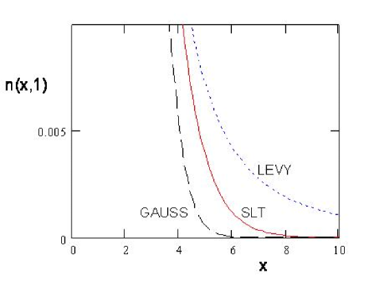
Figure 1: Propagators (Green functions) $G(x)=n(x,t=1)$ for three cases of fractional diffusion. Dotted blue: Lévy superdiffusion ($\alpha=1.5,\ \beta=1$); Solid red: SLT subdiffusion ($\alpha=2,~{}\beta=0.5$), Dashed black: Gaussian diffusion ($\alpha=2,\ \beta=1$).

The asymptotic behavior is most strikingly seen in log-log representation (Fig. 2). The upper reference straight line has a slope [$-(1+\alpha)=-2.5$].

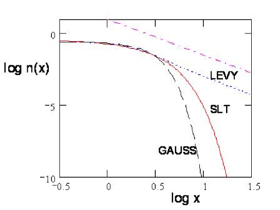
Figure 2: Same data as in Fig. 1, in log-log representation.

We thus see that there are two types of long tails:

• The stretched exponential tail, characteristic, typically, of the subdiffusive  SLT

• The algebraic tail, characteristic of the superdiffusive Lévy process.

Note that both are ”fat” tails, i.e. the decay at large $x$ is slower than the corresponding diffusive Gaussian. The second type is the most slowly decaying one. Warning: it should not be concluded that all subdiffusive processes have exponential tails, whereas all superdiffusive ones have algebraic tails!! (see below).

$\begin{array}[]{l}\mathbf{\alpha=2,\ \ \ \ 1<\beta<2}\end{array}$

This case corresponds to time-fractional superdiffusion. This very interesting case will be treated in detail in Sec. 5.

$\begin{array}[]{l}\mathbf{0<\alpha<2,\ \ \ \ 0<\beta<2}\end{array}$

This is the generic, mixed spatial and temporal fractional diffusion. In this case there is a competition between super- and subdiffusion, expressed by the ratio $2\beta/\alpha$ [see Eq. (26)]. In the work of del-Castillo Negrete et al [16], a model with $\alpha=3/4$, $\beta=0.5$ has been successfully compared with numerical simulations of a set of plasmadynamical equations. In a recent paper [21], additional values of $\alpha<2$ were explored.

In the present work we do not consider the case of space-fractional (Lévy) superdiffusion. We thus fix in all subsequent sections:

$$\alpha=2$$ (46)

4 Random Time-dependent Velocity

We consider a particle moving in one dimension; its position $X(T)$ at time $T$ is determined ”semi-dynamically” by a V-Langevin equation ([2], Ch. 11):

$$\frac{dX(T)}{dT}=V(T),$$ (47)

where the random velocity $V(T)$ (depending solely on time) is defined statistically by specifying the first two moments of the ensemble of its realizations, supposed to be Gaussian, homogeneous and stationary:

$$\left\langle V(T)\right\rangle=0,\ \ \ \ \ \left\langle V(0)~{}V(T)\right\rangle=V_{0}^{2}~{}\mathcal{T}(T).$$ (48)

The function $\mathcal{T}(T)$ need not yet be specified explicitly, except by requiring $\mathcal{T}(0)=1$. $V_{0}$, the initial velocity rms is supposed to be a given parameter.

Let $f(X,T)$ be the (fluctuating) distribution function of the particle. It is represented as usual as:

$$f(X,T)=n(X,T)+\delta f(X,T)$$ (49)

where the ensemble-average $n(X,T)\equiv\left\langle f(X,T)\right\rangle$ is called the density profile, and $\delta f(X,T)$ is the fluctuation. The distribution function obeys the Hybrid Kinetic Equation (HKE):

$$\partial_{T}f(X,T)+V(T)~{}\partial_{X}f(X,T)=0.$$ (50)

The characteristic equation of this first-order partial differential equation coincides with the V-Langevin equation (47). This equation is split, as usual [2], into two components by the averaging operation:

$$\partial_{T}n(X,T)+\partial_{X}~{}\left\langle V(T)~{}\delta f(X,T)\right\rangle=0$$ (51)

$$\partial_{T}\delta f(X,T)+V(T)~{}\partial_{X}~{}\delta f(X,T)+V(T)~{}\partial_{X}~{}n(X,T)-\partial_{X}\left\langle V(T)~{}\delta f(X,T\right\rangle=0$$ (52)

The latter equation is solved by using the propagator:

$$g(X,T|X^{\prime},T^{\prime})=\delta\left[X-X^{\prime}-\int_{T^{\prime}}^{T}dT_{1}~{}V(T_{1})\right]$$ (53)

Substituting its solution into (51), we find:

$$\partial_{T}n(X,T) = \partial_{X}^{2}~{}\int_{0}^{T}dT_{1}~{}\left\langle V(T)V(T_{1})~{}n\left[X-\int_{T_{1}}^{T}dT_{2}~{}V(T_{2}),\ T_{1}\right]\right\rangle$$ (54)

$$+\partial_{X}~{}\left\langle V(T)~{}\delta f\left[X-\int_{0}^{T}dT_{1}V(T_{1}),\ 0\right]\right\rangle$$

This is the exact solution of the problem. It is expressed by an integro-differential equation that is non-local both in time (non-Markovian) and in space (non-local). We do not repeat here the arguments justifying the local approximation, by which the fluctuating displacements $\int_{T_{1}}^{T}dT_{2}~{}V(T_{2}),$ $\int_{0}^{T}dT_{1}~{}V(T_{1})$ in the arguments of $n$ and of $\delta f$ are neglected, and by which the second term of the right hand side, containing the initial fluctuation, is also neglected [2]. The result is an (approximate) local, but non-markovian diffusion equation:

$$\partial_{T}n(X,T)=\partial_{X}^{2}~{}\int_{0}^{T}dT_{1}~{}\left\langle V(T)V(T_{1})\right\rangle~{}n(X,T_{1}).$$ (55)

Using Eq. (48), this becomes:

$$\partial_{T}n(X,T)=\partial_{X}^{2}~{}\int_{0}^{T}dT_{1}~{}V_{0}^{2}~{}\mathcal{T}(T-T_{1})~{}n(X,T_{1}).$$ (56)

Consider, on the other hand, a particle performing a one-dimensional CTRW characterized, in the fluid limit, by a Gaussian jump PDF:

$$\widehat{f}(\kappa)=1-\sigma^{2}~{}\kappa^{2}+...$$ (57)

where $\sigma$ is a characteristic length and $\kappa$ is the dimensional wave vector. The form of the waiting time PDF is not specified at this stage.

The density profile (in F-L representation) obeys Eq. (10) which, written with a dimensional Laplace variable $S$, combined with (57) reduces to:

$$S~{}\widehat{\widetilde{n}}(\kappa,S)-1=-\widetilde{\phi}(S)~{}\sigma^{2}\kappa^{2}~{}\widehat{\widetilde{n}}(\kappa,S)$$ (58)

Its inverse F-L transform is:

$$\partial_{T}n(X,T)=\sigma^{2}~{}\partial_{X}^{2}~{}\int_{0}^{T}dT_{1}~{}\phi(T-T_{1})~{}n(X,T_{1})~{}$$ (59)

This equation constitutes the main result of the first part of our work. Comparing it with Eq. (56), we see that the density profile produced (in the local approximation) by the semi-dynamical V-Langevin equation with a time-dependent $V(t)$, and the density profile produced by a CTRW with $\alpha=2$, - or, more specifically, by the fractional diffusion equation (58) - obey formally identical equations of evolution. This statement will be made more precise in the discussion of Sec. 5. The quantitative correspondence is obtained by identifying the velocity correlation function of the V-Langevin process with the memory function:

$$V_{0}^{2}~{}\mathcal{T}(T)\rightarrow\sigma^{2}~{}\phi(T),$$ (60)

i.e., in F-L representation

$$\widetilde{\mathcal{T}}\mathcal{(S)=}\frac{\sigma^{2}}{V_{0}^{2}}~{}\widetilde{\phi}(S).$$ (61)

We note that Eqs. (56) and (58) were also obtained in Ref. [14] in a quite different manner, which is only valid for the 2-state CTRW. The relation (61) is much more general and was obtained in a simpler direct way.

5 Algebraic Velocity Correlation

We now make the problem explicit, by adopting the same form of the velocity correlation as in Ref. [14]:

$$V_{0}^{2}\mathcal{T}(T)=\frac{A}{T^{\gamma}},\ \ \ \ 0<\gamma<1,$$ (62)

where $A$ is a quantity having dimension [length]²[time]^-2+γ. We then associate with the V-Langevin equation (for $d=1$) (47) [or the Hybrid kinetic equation (50)] a CTRW with memory function given, in the fluid limit, by Eq. (60), leading to the fractional diffusion equation (FDE) (58):

$$S~{}\widehat{\widetilde{n}}(\kappa,S)-1=-A~{}\kappa^{2}~{}S^{\gamma-1}~{}\widehat{\widetilde{n}}(\kappa,S),\ \ \ \ \ ~{}.$$ (63)

This relation agrees with Eq. (33) of [14]. It is trivially equivalent to:

$$S^{2-\gamma}~{}\widehat{\widetilde{n}}(\kappa,S)-S^{1-\gamma}=-A~{}\kappa^{2}~{}\widehat{\widetilde{n}}(\kappa,S)$$ (64)

The F-L density profile is obtained from Eq. (63) in the form:

$$\widehat{\widetilde{n}}(\kappa,S)=\frac{S^{-1-\gamma}}{S^{2-\gamma}+A~{}\kappa^{2}},\ \ \ \ 0<\gamma<1.$$ (65)

Comparing this result with Eq. (16), we immediately see that the two expressions become identical by taking the following value for the waiting time exponent $\beta$:

$$\beta=2-\gamma.$$ (66)

Thus, the process corresponds to time-fractional superdiffusion as defined in Sec. 3:

$$1<\beta<2.$$ (67)

At this point there appears a subtle difficulty (the following argument results from a remark of J. Klafter [22]). The FDE (63) is formally derived as the fluid limit of a CTRW with $\widetilde{\psi}(S)=1-S^{\beta}$, and $\beta$ in the range (66): this is an extension of the range defined in Eq. (13).

The knowledge of the Laplace transform $\widetilde{\psi}(S)$ allows us to calculate the average waiting time between two jumps in the CTRW, by using a well-known formula:

$$\left\langle T\right\rangle=-\left.\frac{\partial\widetilde{\psi}(S)}{\partial S}\right|_{S=0}=\left.\beta~{}S^{\beta-1}\right|_{S=0}$$ (68)

For $0<\beta<1$ the average waiting time of the CTRW is infinite. This denotes a waiting time PDF with a long tail, leading to strange transport, i.e., subdiffusion (Sec. 3 and [2]). For $\beta=1$ the average waiting time is finite, corresponding to normal diffusion.

For $1<\beta<2$, the average waiting time is zero, thus leading to a paradoxical situation. Recalling that $T$ is a semi-definite positive variable, it follows that $\psi(T)\sim\delta(T)$. Thus, any random walker would remain trapped forever at its starting point, in clear contradiction with superdiffusion, as predicted by the diffusion exponent $\mu=2\beta/\alpha=\beta>1$ (Sec. 3). The only other possibility of obtaining a zero average waiting time would be to have $\psi(T)$ negative in part of the range $(0,~{}\infty)$, but then $\psi(T)$ does not qualify for a probability distribution function.

The conclusion of this argument is the following. The function $\widehat{\widetilde{n}}(\kappa,S)$ defined by Eq. (65) is, indeed, the resolvent of the fractional differential equation (FDE) (63), but the latter cannot be derived as the fluid limit of a CTRW.

We are now faced with a new subtlety. The function $\widehat{\widetilde{n}}(\kappa,S)$ is the solution of the linear algebraic equation (64). But, is the latter equation the F-L transform of a fractional diffusion equation? One is tempted to associate Eq. (64) with the FDE in $X-T$ representation:

$${}_{0}^{C}D_{T}^{2-\gamma}n(X,T)=A~{}D_{|X|}^{2}~{}n(X,T),\ \ \ \ \ 0<\gamma<1,$$ (69)

with the initial condition:

$$n(X,0)=\delta(X).$$ (70)

This fractional equation is an ”intermediate” between a diffusion equation ($\gamma=1$) and a wave equation ($\gamma=0$) [23], [8], [10]. But, using the general formula for the Laplace transform of the Caputo fractional derivative [7], [10] and the Appendix of the present paper, the F-L transform of Eq. (69) is:

$$S^{2-\gamma}~{}\widehat{\widetilde{n}}(\kappa,S)-S^{1-\gamma}\widehat{n}(\kappa,T=0)-S^{-\gamma}\widehat{n}_{T}(\kappa,T=0)=-A~{}\kappa^{2}~{}\widehat{\widetilde{n}}(\kappa,S),\ \ \ 0<\gamma<1$$ (71)

It thus appears that the general solution of the Cauchy problem for Eq. (69) requires two initial conditions (like the wave equation): $n(X,0)$ and $n_{T}(X,0)\equiv[\partial n(X,T)/\partial T]_{T=0}$. As a result, the general solution is expressed in terms of two propagators; indeed, the solution of Eq. (71) is:

$$\widehat{\widetilde{n}}(\kappa,S)=\frac{S^{-1-\gamma}}{S^{2-\gamma}+A~{}\kappa^{2}}\widehat{n}(\kappa,0)+\frac{S^{-\gamma}}{S^{2-\gamma}+A~{}\kappa^{2}}\widehat{n}_{T}(\kappa,0).$$ (72)

. We refer to Ref. [10] for a complete solution and discussion of this problem. Here we shall only consider the simpler special case (also considered in [9]):

$$n(X,T=0)=\delta(X),\ \ \ \ n_{T}(X,T=0)=0$$ (73)

$$\widehat{n}(\kappa,T=0)=1,\ \ \ \ \widehat{n}_{T}(\kappa,T=0)=0$$ (74)

In this case, Eq. (71) reduces to Eq. (64), and Eq. (65) represents the F-L propagator of Eq. (69) equipped with the initial conditions (73). The explicit solution for the propagator of (69) (i.e., the F-L inversion of Eq. (65) was obtained analytically by Mainardi [23], [9] (and also by Metzler and Klafter [5] in terms of Fox H-functions):

$$n(X,T;\gamma)=\frac{1}{2\sqrt{A}~{}T^{1-(\gamma/2)}}~{}~{}M_{1-(\gamma/2)}\left(\frac{X}{\sqrt{A}~{}T^{1-(\gamma/2)}}\right),\ \ \ \ \ \ 0<\gamma<1$$ (75)

This has precisely the scaling form (25), with the similarity variable:

$$p=\frac{X}{\sqrt{A}T^{1-(\gamma/2)}}$$ (76)

The special function $M_{1-(\gamma/2)}(p)$ is called the Mainardi function: it is defined for any order $\nu\in(0,1)$ as:

$$M_{\nu}(p)=\sum\limits_{k=0}^{\infty}\frac{(-p)^{k}}{k!~{}\Gamma[-\nu k+(1-\nu)]},\ \ \ 0<\nu<1$$ (77)

This is a special case of a Wright function, defined as follows ([20]):

$$\phi(\alpha,\beta;p)=\sum\limits_{k=0}^{\infty}\frac{p^{k}}{k!~{}\Gamma(\alpha k+\beta)},\ \ \ \ \alpha,~{}\beta~{}>0.$$ (78)

The series (77) is convergent, but the convergence is very slow. In practice, for the numerical calculations displayed below, we take $100$ terms in the series. Mainardi et al 2001 [9] also showed that the asymptotic behavior of the propagator is given by a stretched exponential, which for the value $\beta=2-\gamma$ is:

$$n(X,T;\gamma)=\frac{1}{2\sqrt{A}T^{1-(\gamma/2)}}~{}B~{}p^{a}~{}\exp(-bp^{c}),\ \ \ \ p\gg 1,$$ (79)

with:

$$B = \left[2\pi\gamma~{}2^{(2-\gamma)/\gamma}~{}(2-\gamma)^{2(\gamma-1)/\gamma}\right]^{-1/2},$$

$$a = \frac{1-\gamma}{\gamma},$$

$$b = \gamma\left[\frac{(2-\gamma)^{2-\gamma}}{4}\right]^{1/\gamma}$$

$$c = \frac{2}{\gamma},\ \ \ \ \ \ \ \ \ \ \ \ \ \ \ \ \ \ \ \ \ \ \ \ \ \ \ \ \ \ 0<\gamma<1$$ (80)

The important point here is that the present density profile decays asymptotically according to a stretched exponential law, with exponent $2/\gamma>2$. This implies that the propagator decays asymptotically faster than the Gaussian (contrary to the subdiffusive case $0<\beta<1,$ discussed in Sec.3. Mainardi calls this feature a ”thin tail”. It thus appears clearly that superdiffusion is not necessarily associated with a long (”fat”) tail of the propagator.

Another important property of the propagator (75) [i.e., of the Mainardi function $M_{\nu}(p)$ for $1/2<\nu<1,$ i.e., $1<\beta<2$] is its possessing for $T>0$ two symmetrical maxima that move away from the origin, while becoming wider. As pointed out above, the fractional equation (69), written in a simpler notation ($\partial^{\beta}/\partial T^{\beta}\equiv~{}_{0}^{C}D_{T}^{\beta}$) as:

$$\frac{\partial^{\beta}}{\partial T^{\beta}}n(X,T)=A\nabla^{2}n(X,T),\ \ \ \ \ 1<\beta<2$$ (81)

is a kind of interpolation between a diffusion equation ($\beta=1$) and a wave equation ($\beta=2$). Thus, the solution represents a wave propagating in both directions away from the origin, and damping out on the way . We illustrate these properties by the plot of Fig. 3, corresponding to $\gamma=0.5$, hence $\beta=1.5$. For $T\rightarrow 0$, the propagator tends toward $n(X,0)=\delta(X)$, as it should (70).

Figure 3: Propagator $n(X,T)$ at four different times. $\gamma=0.5,\ A=1.$

We show in Fig. 4 the tail of the propagator (for $T=1$) compared to the tail of the corresponding Gaussian. This situation is to be contrasted with Figs. 1 and 2: both the time-fractional subdiffusive propagator and the space-fractional superdiffusive (Lévy) propagator have ”fat” tails.

Figure 4: Tail of the propagator for $\gamma=0.5$, compared to the corresponding Gaussian packet. $T=1.$

Figs. 3 and 4 allow us to understand how superdiffusion is possible in spite of the thin exponential tail. The dispersion of the matter is produced not only by the broadening of the initial distribution (as in ordinary diffusion) but also by the symmetric wave-like outward motion of the maximum.

The results of the present section are not really new: All these results were also obtained in Ref. [14], using, however, the 2-state model. We showed here that the results are easily extended to an arbitrary fluctuating velocity depending solely on time. Our main result can be summarized as follows.

The motion of a particle in one dimension, with a random velocity depending solely on time, obeying a semi-dynamical V-Langevin equation (V-LE) (47), can be equivalently described by a time-fractional differential equation (FDE). There is, however, no CTRW whose fluid limit is the FDE (74). The V-LE is characterized by a velocity correlation depending (for all positive times!) algebraically on time, $\mathcal{T}(T)\sim T^{-\gamma}$, with an exponent $\gamma\in(0,1)$. The equivalent FDE is characterized by a spatial exponent $\alpha=2$ and a waiting time exponent $\beta=2-\gamma;$ thus $1<\beta<2$. This FDE leads to time-fractional superdiffusion, with diffusion exponent $\mu=2-\gamma>1$. The density profile has two maxima that are moving symmetrically away from each other, while broadening with increasing time. The asymptotic decay is exponential, decreasing faster than a Gaussian in space (”thin tail”).

The model V-LE considered here, though allowing an exact analytical solution, has a physical drawback. The algebraic law of the velocity correlation $\mathcal{T}(T)=T^{-\gamma}$ cannot be valid for short times. For an obvious physical reason, $\underset{T\rightarrow 0}{\lim}\mathcal{T}(T)=1$ [as required by Eq. (48)], instead of diverging as in the present model. The model should certainly be improved by using a correlation function that satisfies this constraint.

We now generalize our model by considering, instead of a velocity depending on a single time variable, a velocity field in two dimensions, for which the velocity depends on both time and space $V(X,T)$.

6 Random Velocity Field with Algebraic Time-correlation

We now return to Eq. (3), and consider a true velocity field, i.e., a function both of space and time. We immediately note that this generalization introduces nothing new in one dimension. We recall the important condition of zero divergence (3) which ensures the correct physical status of the hybrid kinetic equation, i.e., the equivalence of Eqs. (4) and (5). Clearly, the constraint (3) reduces, in one dimension, to $\partial_{X}V(X,T)=0$, hence the velocity can only depend on time, and we are brought back to the situation of Sec. 4. In order to study a non-trivial problem, we must consider $d\geq 2$. Specifically, we shall consider in the rest of the present work two-dimensional systems, $d=2$. As will be shown below, such systems are actually of much greater physical interest than one-dimensional ones.

We thus consider a particle whose position is specified by the vector $\mathbf{X}=(X,Y)$ and the velocity $\mathbf{V}=(V_{x},V_{y})$. The corresponding (vectorial) V-Langevin equation is:

$$\frac{d\mathbf{X}(T)}{dT}=\mathbf{V[X}(T),T],\ \ \ \ \ \ \ \ \mathbf{X}(0)=\mathbf{0}.$$ (82)

As a result of the previous discussion, we may associate with this V-Langevin equation a hybrid kinetic equation, provided that the velocity field has zero divergence:

$$\mathbf{\nabla\cdot V(X},T)\equiv\partial_{X}V_{x}(\mathbf{X},T)+\partial_{Y}V_{y}(\mathbf{X},T)=0.$$ (83)

Contrary to the one-dimensional case, this condition can be realized with a non-trivial velocity field. The associated hybrid kinetic equation possesses both required properties: it conserves the normalization of $f$ and its characteristic equations are Eqs. (82). Thus, the two following forms are equivalent:

$$\partial_{T}f(\mathbf{X},T)+\mathbf{\nabla\cdot}\left[\mathbf{V(X},T)~{}f(\mathbf{X},T)\right]=0,$$ (84)

$$\partial_{T}f(\mathbf{X},T)+\mathbf{V(X},T)\cdot\mathbf{\nabla}f(\mathbf{X},T)=0$$ (85)

We note that the condition of zero divergence of a two-dimensional velocity field is realized, in particular, by the intensely studied model of a charged particle moving perpendicularly to a strong constant magnetic field $\mathbf{B}$, in presence of a fluctuating electrostatic field (see, e.g. [2], where many other references are given]. The coordinates of its guiding centre are animated by the well-known electrostatic drift velocity (in Gaussian units):

$$\frac{dX(T)}{dT} = -\frac{c}{B}~{}\left.\frac{\partial\Phi[X,Y,T]}{\partial Y}\right|_{\mathbf{X=X(}T)},$$

$$\frac{dY(T)}{dT} = \frac{c}{B}~{}\left.\frac{\partial\Phi[X,Y,T]}{\partial X}\right|_{\mathbf{X=X(}T)},$$ (86)

where $\Phi(\mathbf{X},T)$ is the (fluctuating) scalar potential. The statistical properties of the velocity field are thus derived from the statistical definition of the potential. We assume that the latter is a Gaussian centred, homogeneous, isotropic and stationary random process, defined by a vanishing first moment and by the following factorized form of the second moment:

$$\left\langle\Phi(\mathbf{X},T)\right\rangle = 0,$$

$$\left\langle\Phi(\mathbf{0},0)~{}\Phi(\mathbf{X},T)\right\rangle = \mathcal{E}(\mathbf{X})~{}\mathcal{T}(T).$$ (87)

The second relation defines the Eulerian potential correlation, i.e., the correlation between the values of the potential at the origin and at a fixed point $\mathbf{X}$ at time $T$. In the present work we consider only the case where the spatial part of the correlation has a Gaussian form:

$$\mathcal{E}(\mathbf{X})=\exp\left(-\frac{X^{2}+Y^{2}}{2\lambda^{2}}\right),$$ (88)

where $\lambda$ is the so-called correlation length. The temporal part $\mathcal{T}(T)$ will not yet be specified explicitly. It should, however, satisfy the condition: $\mathcal{T}(0)=1$, and is supposed to depend only on the absolute value of $T$.

It is convenient to introduce from here on dimensionless quantities (denoted by lower case letters), defined as follows:

$$x=\frac{X}{\lambda},\ \ y=\frac{Y}{\lambda},\ \ t=\frac{T}{T_{c}},\ \ \phi=\varepsilon^{-1}\Phi.$$ (89)

Here $\varepsilon$ is a measure of the intensity of the potential fluctuations, e.g., the root mean square value of the potential fluctuations. $T_{c}$ is an intrinsic characteristic time, to be defined later [Sec. 8]. The V-Langevin equations of motion (86) reduce to:

$$\frac{d\mathbf{x}(t)}{dt}=K~{}\mathbf{v[x}(t),t],$$

$$v_{x}(\mathbf{x},t)=-\frac{\partial\phi(\mathbf{x},t)}{\partial y},\ \ \ v_{y}(\mathbf{x},t)=\frac{\partial\phi(\mathbf{x},t)}{\partial x}.$$ (90)

The dimensionless constant $K$ is called the Kubo number:

$$K=\frac{c}{B}~{}\frac{\varepsilon T_{c}}{\lambda^{2}}.$$ (91)

Given the form of Eqs. (90) it is even more convenient to use a further reduction of the time variable:

$$\theta=Kt.$$ (92)

The V-Langevin equations then reduce to:

$$\frac{d\mathbf{x}(\theta)}{d\theta}=\mathbf{v[x}(\theta),\theta],\ \ \ \ \mathbf{x}(0)=\mathbf{0}.$$ (93)

The relevant dimensionless Eulerian correlations are now defined as follows:

$$\left\langle\phi(\mathbf{0},0)~{}\phi(\mathbf{x,}\theta)\right\rangle = \mathcal{E(}\mathbf{x)~{}}\mathcal{T(}K^{-1}\theta),$$

$$\left\langle v_{j}(\mathbf{0},0)~{}v_{n}(\mathbf{x,}\theta)\right\rangle = \mathcal{E}_{jn}\mathcal{(}\mathbf{x)~{}}\mathcal{T(}K^{-1}\theta),$$ (94)

with (88):

$$\mathcal{E}_{xx}(x,y) = -\frac{\partial^{2}}{\partial y^{2}}\mathcal{E}(x,y)=(1-y^{2})\mathcal{E}(x,y),$$

$$\mathcal{E}_{yy}(x,y) = -\frac{\partial^{2}}{\partial x^{2}}\mathcal{E}(x,y)=(1-x^{2})\mathcal{E}(x,y),$$

$$\mathcal{E}_{xy} = \mathcal{E}_{yx}=\frac{\partial^{2}}{\partial x\partial y}\mathcal{E(}x,y)=xy\mathcal{E(}x,y).$$ (95)

A first, well-known general result is obtained from the V-Langevin equation (93): the mean square deviation (MSD) in the $x$-direction is expressed as follows:

$$\left\langle x^{2}(\theta\right\rangle=2\int_{0}^{\theta}d\tau~{}(\theta-\tau)~{}\mathcal{L}_{xx}(\tau).$$ (96)

Here $\mathcal{L}_{xx}(\theta)$ is the Lagrangian velocity correlation, calculated along the trajectory $\mathbf{x}(\theta)$ of the particle, i.e., using the solution of Eq. (93):

$$\mathcal{L}_{xx}(\theta)=\left\langle v_{x}(\mathbf{0},0)~{}v_{x}[\mathbf{x}(\theta),\theta]\right\rangle.$$ (97)

The MSD is related to the dimensionless running diffusion coefficient $\mathcal{D}_{x}(\theta)$ in the $x$-direction by the well-known Einstein relation:

$$\mathcal{D}_{x}(\theta)=\frac{1}{2}~{}\frac{d\left\langle x^{2}(\theta)\right\rangle}{d\theta}=\int_{0}^{\theta}d\tau~{}\mathcal{L}_{xx}(\tau).$$ (98)

We now consider the evolution of the density profile $n(\mathbf{x},\theta)=\left\langle f(\mathbf{x,}\theta\right\rangle$. The distribution function is governed by the hybrid kinetic equation (84), or equivalently, (85). The latter is treated by a straightforward generalization of the reasoning leading from Eq. (50) to (55); it will not be repeated here. The final result differs from the latter equation in that the simple one-dimensional velocity correlation $\left\langle v(\theta_{1})~{}v(\theta)\right\rangle$ is replaced by the Lagrangian velocity correlation tensor $\left\langle v_{j}[\mathbf{x}(\theta_{1}),\theta_{1}]~{}v_{k}[\mathbf{x}(\theta),\theta]\right\rangle=\mathcal{L}_{jk}(\theta-\theta_{1})$:

$$\partial_{\theta}n(\mathbf{x},\theta)=\nabla_{j}\int_{0}^{\theta}d\tau~{}\mathcal{L}_{jk}(\tau)~{}\nabla_{k}~{}n(\mathbf{x},\theta-\tau).$$ (99)

Clearly, the relation (96) can be obtained directly from Eq. (99).

7 The Corrsin Approximation

The study of transport is now reduced to the (difficult) determination of the Lagrangian velocity correlation. More precisely, we want to find a relation between the (given) Eulerian velocity correlation and the Lagrangian one. In the present work we will use only the simplest approximation method for this problem: the Corrsin approximation [24], [2].

We rewrite the exact Lagrangian velocity correlation as follows:

$$\mathcal{L}_{jn}(\theta)=\left\langle v_{j}(\mathbf{0},0)~{}v_{n}[\mathbf{x}(\theta),\theta]\right\rangle$$

$$=\int d\mathbf{x}~{}\left\langle v_{j}(\mathbf{0},0)~{}v_{n}(\mathbf{x},\theta)~{}\delta[\mathbf{x}-\mathbf{x}(\theta)]\right\rangle$$ (100)

In the Corrsin approximation, the average in the integrand is assumed to be factorized as follows:

$$\mathcal{L}_{jn}(\theta)\approx\int d\mathbf{x}~{}\left\langle v_{j}(\mathbf{0},0)~{}v_{n}(\mathbf{x},\theta)\right\rangle~{}~{}\left\langle\delta[\mathbf{x}-\mathbf{x}(\theta)]\right\rangle$$ (101)

The first factor in the integrand is recognized as the Eulerian correlation tensor, assumed to be of the form (87), thus:

$$\mathcal{L}_{jn}(\theta)\approx\int d\mathbf{x}~{}\mathcal{E}_{jn}(\mathbf{x})~{}\mathcal{T}(\theta/K)~{}\left\langle\delta[\mathbf{x}-\mathbf{x}(\theta)]\right\rangle.$$ (102)

The last factor is evaluated as follows, in the second cumulant approximation:

$$\left\langle\delta[\mathbf{x}-\mathbf{x}(\theta)]\right\rangle = \int d\mathbf{k}~{}e^{i\mathbf{k\cdot x}}~{}\left\langle e^{-i\mathbf{k\cdot x}(\theta)}\right\rangle$$ (103)

$$\approx \int d\mathbf{k}~{}e^{i\mathbf{k\cdot x}}~{}\exp\left[-~{}\tfrac{1}{2}~{}k^{2}\left\langle x^{2}(\theta)\right\rangle\right]$$

$$= \frac{1}{2\pi~{}\left\langle x^{2}(\theta)\right\rangle}~{}\exp\left[-~{}\frac{x^{2}+y^{2}}{2~{}\left\langle x^{2}(\theta)\right\rangle}\right].$$

Thus:

$$\mathcal{L}_{jn}(\theta)=\frac{\mathcal{T}(\theta/K)}{2\pi~{}\left\langle x^{2}(\theta)\right\rangle}~{}\int d\mathbf{x}~{}\mathcal{E}_{jn}(\mathbf{x})\exp\left[-~{}\frac{x^{2}+y^{2}}{2~{}\left\langle x^{2}(\theta)\right\rangle}\right].$$ (104)

We now use the explicit forms (95) for the Eulerian correlation. It is immediately seen by symmetry that the non-diagonal components of the Lagrangian tensor vanish, and the two diagonal ones are equal to each other.

$$\mathcal{L}_{jn}(\theta)=\delta_{jn}~{}\mathcal{L}(\theta),$$ (105)

with:

$$\mathcal{L}(\theta)=\frac{\mathcal{T}(\theta/K)}{2\pi\left\langle x^{2}(\theta)\right\rangle}~{}\int dx~{}dy~{}(1-y^{2})~{}\exp\left[-\left(1+\frac{1}{\left\langle x^{2}(\theta)\right\rangle}\right)\frac{x^{2}+y^{2}}{2}\right].$$

The integration over $x$ and $y$ is elementary. The result is combined with Eq. (96) to yield:

$$\mathcal{L}(\theta)=\frac{\mathcal{T}(\theta/K)}{\left[1+2\int_{0}^{\theta}d\tau~{}(\theta-\tau)~{}\mathcal{L}(\tau)\right]^{2}}$$ (106)

We thus ended with an integral equation for the Lagrangian velocity correlation in the Corrsin approximation [26], [2]. This equation will be solved in Secs. 9 and 10.

The diagonal character of the Lagrangian velocity correlation introduces a significant simplification in the equation for the density profile, which reduces to the following non-Markovian diffusion equation:

$$\partial_{\theta}n(\mathbf{x},\theta)=\int_{0}^{\theta}d\tau~{}\mathcal{L}(\tau)~{}\nabla^{2}n(\mathbf{x},\theta-\tau).$$ (107)

The diffusion coefficients in the $x$- and $y$-directions are equal to each other. We may therefore drop the subscripts in Eq. (98) and write simply:

$$\mathcal{D}(\theta)=\int_{0}^{\theta}d\tau~{}\mathcal{L}(\tau).$$ (108)

Whenever this integral converges, its limit for $\theta\rightarrow\infty$ defines the ordinary diffusion constant: $\mathcal{D=D}(\infty)$. Whenever $\mathcal{D}$ is finite and positive, the regime is normal diffusive.

8 Algebraic Time Correlation: General Properties

We now make the problem more explicit. We consider a class of V-Langevin equations (and associated hybrid kinetic equations) for which the temporal part of the Eulerian velocity correlation, $\mathcal{T}(\theta/K)$, is a long-tailed function that decays algebraically for long times. It is of the general form (62), but we take now some additional precautions to ensure a correct behavior at short times. We must, in particular, avoid the divergence at $T\rightarrow 0$. Physically, any correct (dimensional) correlation function should have the property: $\mathcal{T}(T=0)=1$. We thus define a characteristic cut-off time $T_{c}$ as the value of $T$ at which the right hand side of Eq. (62) equals $1$. For all times $0\leq T\leq T_{c}$ we put $\mathcal{T}(T)=1$. Note that a correlation of the form (62) has no intrinsic time scale; but the adoption of a cut-off introduces a characteristic time $T_{c}$. The latter allows us to complete the definitions of the dimensionless time $t=T/T_{c}$ (89), of the Kubo number (91) and of the dimensionless variable $\theta$ (92). We thus adopt the final form of the dimensionless temporal Eulerian velocity correlation as:

$$\mathcal{T(}K^{-1}\theta)=\left\{\begin{array}[]{c}1,\ \ \ \ \ 0\leq\theta\leq K\\ \dfrac{K^{\gamma}}{\theta^{\gamma}},\ \ \ \ \ \theta\geq K{}{}\end{array}\right.,\ \ \ 0<\gamma<1$$ (109)

For convenience, $\gamma$ will be called the Eulerian exponent; by definition it will be limited to the range ($0,1$). Anticipating the results of the next Section, it will be shown that the Lagrangian correlation function $\mathcal{L}(\theta)$ has the same general algebraic form, with different values of the exponent and of the coefficients:

$$\mathcal{L(}\theta)=\left\{\begin{array}[]{c}1,\ \ \ \ \ \ \ \ \ \ \ \ \ \ \ \ \ 0\leq\theta\leq\theta_{L},\\ \dfrac{h}{\theta^{\Lambda}},\ \ \ h>0,\ \ \ \ \ \theta>\theta_{L}.{}{}\end{array}\right.$$ (110)

In order to ensure a correct connection of the two parts, we must take:

$$\theta_{L}=h^{1/\Lambda}.$$ (111)

$\Lambda$ will be called the Lagrangian exponent: its value depends on the Eulerian exponent $\gamma$ and on $K$. It will be determined in the next sections.

Before going into specific calculations, we wish to derive an important property relating the nature of the macroscopic transport to the value of the Lagrangian exponent. Combining the definition of the dimensionless running diffusion coefficient (108) with the form (110) we obtain:

$$\mathcal{D}(\theta)=\left\{\begin{array}[]{c}\int_{0}^{\theta}d\tau~{}1,\ \ \ \ \ \ \ \ \ \ \ \ \ \ \ \ \ \ 0\leq\theta\leq\theta_{L},\\ \int_{0}^{\theta_{L}}d\tau~{}1+\int_{\theta_{L}}^{\theta}d\tau~{}h~{}\theta^{-\Lambda},\ \ \ \ \theta>\theta_{L}.\end{array}\right.$$ (112)

The integrals are easily evaluated:

$$\mathcal{D(\theta)=}\left\{\begin{array}[]{c}\theta,\ \ \ \ \ \ \ \ \ \ \ \ \ \ \ \ \ \ \ \ \ \ \ \ \ \ \ \ \ \ \ \ \ \ \ \ \ \ 0\leq\theta\leq\theta_{L,}\\ \theta_{L}+\dfrac{h}{1-\Lambda}\left(\theta^{-\Lambda+1}-\theta_{L}^{-\Lambda+1}\right),\ \ \ \ \theta>\theta_{L}.\end{array}\right.,\ \ \ \Lambda\neq 1.$$ (113)

The more interesting long-time part is rewritten as the sum of a constant and of a time-dependent term; using also Eq. (111) we find:

$$\mathcal{D}(\theta)=\frac{\Lambda}{\Lambda-1}~{}h^{1/\Lambda}+\frac{h}{1-\Lambda}~{}\theta^{1-\Lambda},\ \ \ \ \ \ \theta>\theta_{L},\ \ \ \ \Lambda\neq 1.$$ (114)

We now see the existence of two sharply separated ranges of the Lagrangian correlation exponent $\Lambda.\vskip 12.0pt plus 4.0pt minus 4.0pt$

A) $\mathbf{0<\Lambda<1}$. In this case the second term in the right hand side of (114) is a monotonically increasing function of time. Hence, for sufficiently long times this term strongly dominates the first constant term, and the running diffusion coefficient behaves asymptotically as:

$$\mathcal{D}(\theta)\underset{\theta\rightarrow\infty}{\sim}\theta^{1-\Lambda},\ \ \ \ \ \Lambda<1.$$ (115)

The regime is thus (time-fractional) superdiffusive.

B) $\mathbf{\Lambda=1.}$ Eq. (113) is no longer valid, but the integral in (112) can be evaluated as:

$$\mathcal{D}(\theta)=h^{1/\Lambda}+h~{}\ln\left(\frac{\theta}{h^{1/\Lambda}}\right),\ \ \ \ \Lambda=1.$$ (116)

The regime is ”weakly superdiffusive”.

C) $\mathbf{\Lambda>1}$. The behavior is radically different. The second term in the right hand side of Eq. (114) is now a monotonically decreasing function of time. For long times this term decreases to zero. Hence the running diffusion coefficient tends toward a positive constant:

$$\mathcal{D(\theta)}\underset{\theta\rightarrow\infty}{\sim}\mathcal{D}=\frac{\Lambda}{\Lambda-1}~{}h^{1/\Lambda}>0,\ \ \ \ \ \Lambda>1.$$ (117)

The regime is now normal diffusive for all values of $\Lambda>1$. The asymptotic $\mathcal{D}$ is the ordinary diffusion constant.

Clearly, the value $\Lambda=1$ is a very special one: as $\Lambda$ reaches $1$ from below, the regime changes abruptly from a superdiffusive to a normal diffusive one, and remains so for all values of $\Lambda>1$. This phenomenon is illustrated in Fig. 5.

Figure 5: Running diffusion coefficient $\mathcal{D}(\theta,\Lambda)$ obtained from the kinetic equation, for various values of $\Lambda<1$ and $\Lambda>1$.

The difference between the normal diffusive regime obtained from the kinetic equation and the subdiffusive regime predicted by the CTRW for the same value of $\Lambda>1$ appears clearly in Fig. 6.

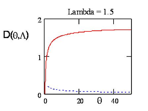
Figure 6: Running diffusion coefficient for $\Lambda=1.5$, as obtained from the kinetic equation (solid red) and as predicted from the CTRW (dotted blue).

In order to obtain a clearer picture of what happens at this point, we study the density profile. More specifically, we investigate whether its evolution can be described by an equivalent FDE, as was found in Sec. 2.

As shown in Sec. 4, there exists a formal equivalence between, on one hand, the non-Markovian diffusion equation (107) obtained from the hybrid kinetic equation and on the other hand, the Montroll-Shlesinger equation for a CTRW in the fluid limit. It requires the identification (60) of the Lagrangian velocity correlation with the memory function of the CTRW (in dimensionless variables):

$$\mathcal{L}(\theta)\rightarrow\phi(\theta),$$ (118)

or, in Laplace representation:

$$\widetilde{\mathcal{L}}(s)\rightarrow\widetilde{\phi}(s).$$ (119)

The Laplace transform of the Lagrangian correlation (110) is, for long times:

$$\widetilde{\mathcal{L}}(s)\sim s^{\Lambda-1}.$$ (120)

Comparing with Eq. (14) we find that the temporal exponent of the ”formally equivalent” FDE is:

$$\beta=2-\Lambda.$$ (121)

Substituting this value into Eq. (16) we find a result similar to (65), with $\Lambda$ replacing $\gamma.$ The resolvent given by the Montroll-Weiss equation is:

$$\widehat{\widetilde{n}}(k,s)=\frac{s^{1-\Lambda}}{s^{2-\Lambda}+\frac{1}{2}k^{2}}$$ (122)

The difference with (65) is that we should not limit consideration to $\Lambda<1$. We consider, instead the various cases discussed above.

A) $\mathbf{0<\Lambda<1}$. The situation is the same as in Sec. 5. There is indeed a complete identity between the kinetic result and the FDE with $2-\Lambda$, i.e., $1<\beta<2$. As shown, however, in Sec. 5, there is no equivalent CTRW in this case. The regime is one of time-fractional superdiffusion. The density profile is provided explicitly by the Mainardi function (75). It has two moving maxima, as represented in Fig. 3 and decays asymptotically as a stretched exponential. The diffusion exponent $\mu=2-\Lambda$. All this is in agreement with the kinetic result.

B) $\mathbf{\Lambda=1}$. The resolvent (122) of the FDE reduces to:

$$\widehat{\widetilde{n}}(k,s)=\frac{1}{s+k^{2}},\ \ \ \ (\Lambda=1)$$ (123)

This is the Fourier-Laplace transform of a Gaussian packet, characteristic of a normal diffusive regime. On the other hand, the result (116) shows that the running diffusion coefficient obtained from the kinetic equation grows, slowly but indefinitely in time. The FDE is no longer equivalent to kinetic theory: $\Lambda=1$ appears as a bifurcation point.

C) $\mathbf{1<\Lambda<2}$. The propagator (122) corresponds now to a FDE with $\alpha=2,\ 0<\beta<1$. It describes a time-fractional subdiffusion, which can be derived as the fluid limit of a CTRW. The corresponding propagator has a single maximum at the origin, and decays according to a stretched exponential [see Eq. (42)]. This regime has been studied in detail in [2]. On the other hand, the kinetic theory predicts a normal diffusive regime throughout this range of $\Lambda$ [Eqs. (114), (117)]. There appears now a divorce between CTRW, FDE and kinetic theory. $\Lambda=1$ has indeed the property of a bifurcation point: as the parameter $\Lambda$ increases from $0$; the propagator first follows the ”FDE branch”. At $\Lambda=1$ it leaves this branch and follows the completely different ”diffusive branch”.

The kinetic equation for the propagator in this regime is obtained from Eqs. (99) and (110):

$$\partial_{\theta}n(x,\theta)=\theta_{L}\nabla^{2}n(x,\theta)+~{}h\int_{\theta_{L}}^{\theta}d\tau~{}\tau^{-\Lambda}~{}\nabla^{2}n(x,\theta-\tau),\ \ \ \theta>\theta_{L}$$ (124)

For long enough time, the equation can be Markovianized by neglecting the retardation in the right hand side. This approximation is justified by our knowledge that a constant diffusion coefficient exists. The final asymptotic equation is an ordinary diffusion equation:

$$\partial_{\theta}n(x,\theta)=\mathcal{D}~{}\nabla^{2}n(x,\theta),$$ (125)

with $\mathcal{D}$ given by Eq. (117). Nevertheless, for any finite time this Markovianization is not reliable, because of the non-exponential Lagrangian correlation, hence the density profile is in general non-Gaussian.

D) $\mathbf{\Lambda>2.}$ In this range the divorce between kinetic theory and FDE is complete. The latter looses its meaning. Indeed, it would correspond to $\beta<0$, which would describe a waiting time distribution that is an increasing function of time. Alternatively, its Laplace transform diverges: $\widetilde{\psi}(s)\sim s^{-|\beta|}\rightarrow\infty$ as $s\rightarrow 0$. On the other hand, the Markovianization of the kinetic equation (124) is more and more justified as $\mathcal{L}(\theta)$ decreases faster for large $\theta$.

9 Lagrangian Velocity Correlation:
 First Approximation

We now determine the Lagrangian velocity correlation as a function of time and of the parameters $\gamma$ and $K$ of the input Eulerian velocity correlation, by solving the integral equation (106). The procedure used is one of successive numerical iterations $\mathcal{L}^{(n)}(\theta)$, starting with the natural Eulerian trial function $\mathcal{L}^{(0)}(\theta)=\mathcal{T}(\theta/K)$. We checked the convergence of the procedure. As can be seen in Fig. 7, the second iteration provides already an excellent approximation.

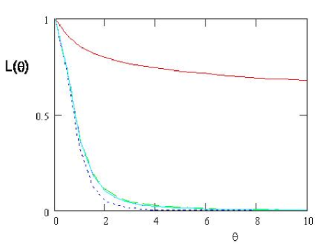
Figure 7: Solution of Eq. (106) for the Lagrangian velocity correlation. Red solid: starting (Eulerian) correlation; Blue dotted: First iteration. The second, third and fourth iterations are superposed on the green curve. The parameters are: $K=0.2$, $\gamma=0.1.$

The first very important qualitative result is the following. An input Eulerian correlation (109) with an algebraic tail produces a Lagrangian correlation having the same type of algebraic tail. This is clearly seen in a log-log representation of the result, as shown in Fig. 8. We thus confirm the anticipated form (111). Our main task will be the determination of the Lagrangian exponent $\Lambda$, of the corresponding ”intensity” $h$ and of the cut-off time $\theta_{L}$ as functions of the input Eulerian exponent $\gamma$ and of the Kubo number $K$.

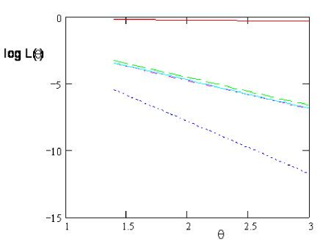
Figure 8: Same data as in Fig. 7, in log-log representation.

A first glance at Fig. 7 shows that, even for relatively small values of $K$, the Lagrangian correlation deviates very quickly from the Eulerian one: this is clearly seen in Fig. 8. Thus, the nonlinearity, measured by $K,$ is far from producing just a small perturbation.

Figure 9: First iterate of the Lagrangian velocity correlation $\mathcal{L}^{(1)}(\theta)$, (solid red) compared to the Eulerian correlation $\mathcal{T(\theta)}$ (dotted blue) at short times. $K=0.5,\ \gamma=0.1.$

The first iteration is not quantitatively accurate (Fig. 7), but it has the advantage that it can be evaluated analytically. It is therefore interesting to study explicitly some of its properties which provide a global qualitative picture. The explicit form is (106):

$$\mathcal{L}^{(1)}(\theta)=\frac{\mathcal{T(\theta}/K)}{\left[1+2\int_{0}^{\theta}d\tau~{}(\theta-\tau)~{}\mathcal{T}(\tau/K)\right]^{2}}.$$ (126)

The integral in the denominator, combined with the definition (109), can be written in terms of two other integrals as follows:

$$\int_{0}^{\theta}d\tau~{}(\theta-\tau)~{}\mathcal{T}(\tau/K)=\left\{\begin{array}[]{c}I_{1}(\theta),\ \ \ \ \ \ \ \ \ \ \ \ \theta<K\\ I_{1}(K)+I_{2}(\theta),\ \ \ \ \ \theta>K\end{array}\right.$$ (127)

where:

$$I_{1}(\theta)=\int_{0}^{\theta}d\tau~{}(\theta-\tau)=\tfrac{1}{2}~{}\theta^{2},$$ (128)

$$I_{2}(\theta)=\int_{K}^{\theta}d\tau~{}(\theta-\tau)~{}\frac{K^{\gamma}}{\tau^{\gamma}}$$

$$=\frac{1}{(1-\gamma)(2-\gamma)}~{}K^{\gamma}\theta^{2-\gamma}-\frac{1}{1-\gamma}~{}K\theta+\frac{1}{2-\gamma}~{}K^{2}.$$ (129)

Combining these partial results, we finally obtain:

$$\mathcal{L}^{(1)}(\theta)=\left(1+\theta^{2}\right)^{-2},\ \ \ \ \ \ \theta<K,$$ (130)

$$\mathcal{L}^{(1)}(\theta) = \dfrac{K^{\gamma}}{\theta^{\gamma}\left[1+\dfrac{2}{(1-\gamma)(2-\gamma)}K^{\gamma}\theta^{2-\gamma}-\dfrac{2}{(1-\gamma)}K\theta+\dfrac{4-\gamma}{(2-\gamma)}K^{2}\right]^{2}},\ \ \ \theta>K.$$

The behavior of this function for short times is very simple: starting from $1$, it decreases parabolically:

$$\mathcal{L}^{(1)}(\theta)\sim 1-2\theta^{2},\ \ \ \ \theta\ll K$$ (132)

As $\theta$ reaches $K$, we find, of course, that the two branches (130) and (LABEL:eeq.131) join each other at the same point. But the derivative at $\theta=K$ is discontinuous. Indeed, consider the two integrals (128) and (129); one easily finds:

$$\left.\frac{d}{d\theta}I_{1}(\theta)\right|_{\theta=K}=K,\ \ \ \ \ \left.\frac{d}{d\theta}I_{2}(\theta)\right|_{\theta=K}=0.$$

Thus, $\mathcal{L}^{(1)}(\theta)$ exhibits a kink at $\theta=K$, as can be seen in Fig. 9.

The asymptotic behavior for large $\theta$ is more interesting. Here we must distinguish two ranges of the Eulerian exponent $\gamma$.

a) $\mathbf{\gamma<1}$. In this case the term proportional to $\theta^{2-\gamma}$ dominates all others in the denominator of Eq. (LABEL:eeq.131) for large $\theta$. We thus find:

$$\mathcal{L}^{(1)}(\theta)\sim\frac{K^{\gamma}}{\theta^{\gamma}~{}\frac{4}{(1-\gamma)^{2}(2-\gamma)^{2}}~{}K^{2\gamma}\theta^{4-2\gamma}}.$$

We thus find, indeed, for very small $\gamma$, an algebraic tail of the form (110):

$$\mathcal{L}^{(1)}(\theta)\sim\frac{h^{(1)}(K,\gamma)}{\theta^{4-\gamma}},\ \ \ \theta\gg K,\ \ \ \ \gamma\ll 1,$$ (133)

with:

$$h^{(1)}(K,\gamma)=\left[\frac{(1-\gamma)(2-\gamma)}{2}\right]^{2}K^{-\gamma}.$$ (134)

Next, we note that the Lagrangian exponent in this approximation is:

$$\Lambda^{(1)}(\gamma)=4-\gamma,\ \ \ \gamma\ll 1$$ (135)

Although this value is not accurate (as can be seen from Fig. 8), it has the important property (which will be confirmed) that it only depends on $\gamma$, not on $K$ (for very small $\gamma)$.

b) $\mathbf{\gamma>1}$. In this case the dominant term at large $\theta$ in the denominator of Eq. (LABEL:eeq.131) is the term proportional to $\theta$. The asymptotic behavior is thus different:

$$\mathcal{L}^{(1)}(\theta)\sim\frac{K^{\gamma}}{\theta^{\gamma}~{}\frac{4}{(1-\gamma)^{2}}~{}K^{2}\theta^{2}},$$

hence:

$$\mathcal{L}^{(1)}(\theta)\sim\frac{k^{(1)}(K,\gamma)}{\theta^{2+\gamma}},\ \ \ \ \theta\gg K,\ \ \ \ \gamma\gg 1,$$ (136)

where $k^{(1)}(K,\gamma)$ is found from this equation. The important point is that the Lagrangian exponent takes a different dependence on $\gamma$ for larger values of this exponent:

$$\Lambda^{(1)}(\gamma)\sim 2+\gamma,\ \ \ \ \ \ \gamma\gg 1.$$ (137)

Thus, $\Lambda^{(1)}(\gamma)$, which was a decreasing function, starts increasing with $\gamma$ beyond $\gamma=1$. We may calculate analytically the exact dependence of $\Lambda^{(1)}(\gamma)$ by evaluating the slope of the log-log graph of $\mathcal{L}^{(1)}(\theta)$ (see Fig. 8):

$$\Lambda^{(1)}(\gamma)=\log[\mathcal{L}^{(1)}(100,K,\gamma)]-\log[\mathcal{L}^{(1)}(1000,K,\gamma)]$$ (138)

The result is shown in Fig. 10. Comparing this type of figures for different values of $K$, one finds a very weak dependence of $\Lambda$ on $K$ for $\gamma$ close to $1$.

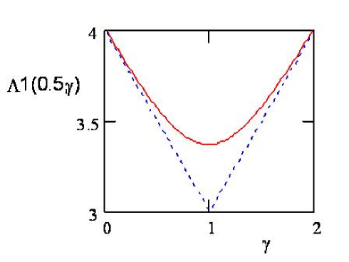
Figure 10: Lagrangian exponent in the first iteration, as a function of the Eulerian exponent $\gamma.$ $K=0.5$. The left (right) dotted straight lines correspond to Eqs. ( 135) [resp. (137)].

The important consequence of this new ”bifurcation” is the fact that, for all values of $\gamma$ we find:

$$\Lambda^{(1)}(\gamma)>3,\ \ \ \ \ \forall\gamma.$$ (139)

The first iteration thus predicts, in accordance with the discussion at the end of Sec. 8, that the first iterate of the Lagrangian correlation leads to a diffusive regime for all values of $\gamma$. More than that: the Lagrangian exponent is in the range D), where there is no equivalence between kinetic theory and CTRW or FDE. This statement, however, has to be confirmed by the final solution.

10 Lagrangian Velocity Correlation. Final Numerical Calculation.

As shown in the previous section, the second iterate of Eq. (106) yields already an excellent approximation, while not requiring long numerical calculations (we therefore omit the superscript ${}^{(2)})$.The short-time ($\theta<K$) part can even be calculated analytically. We thus have:

$$\mathcal{L(\theta)=}\frac{1}{(1+\theta\arctan\theta)^{2}},\ \ \ \ \theta<K,$$ (140)

$$\mathcal{L}(\theta)=\frac{K^{\gamma}}{\theta^{\gamma}\left[1+K\arctan K+2\int_{K}^{\theta}d\tau~{}(\theta-\tau)~{}\mathcal{L}^{(1)}(\tau)\right]^{2}},\ \ \ \ \theta>K.$$ (141)

Eq. (LABEL:eeq.131) is substituted in the integral, and the expression is evaluated numerically.

For short times, the Lagrangian correlation behaves as:

$$\mathcal{L}(\theta)\sim(1+\theta^{2})^{-2}\sim 1-2\theta^{2},\ \ \ \ \ \theta\ll K,$$ (142)

i.e., exactly as in the first approximation (132). As can be seen in Fig. 11, the kink which appeared at $\theta=K$ in the first approximation is still present in the final expression.

Figure 11: Second iterate of the Lagrangian velocity correlation $\mathcal{L}^{(2)}(\theta)=\mathcal{L}(\theta)$, (solid red) compared to the first iterate $\mathcal{L}^{(1)}(\theta)$ (dashed green) and to the Eulerian correlation $\mathcal{T(\theta)}$ (dotted blue) at short times. $K=0.5,\ \gamma=0.1.$

The long-time behavior is, of course, more interesting. The first important point, that is seen in Fig. 8, is that the Lagrangian velocity correlation behaves asymptotically as a power law, (110), thus confirming our previous anticipation. We now study its parameters.

The Lagrangian exponent $\Lambda$ is in all cases smaller than the one given by the first iterate, but much larger than the Eulerian exponent $\gamma$, as seen in Fig. 8. In Fig. 12 we plotted $\log\mathcal{L}(\theta)$ vs $\log\theta$ for given $\gamma=0.1$ and three values of $K=0.1,~{}0.5,0.7$. For all these relatively small values of $K$ the exponent $\Lambda$ is strictly the same: $\Lambda(\gamma=0.1)=2.10,$ $\forall K$.

Figure 12: Lagrangian velocity correlation vs. $\theta$, in log-log representation. The curves correspond to $K=0.1$ (solid red), $K=0.5$ (dotted blue) and $K=0.7$ (dashed green). $\gamma=0.1.$

Next, we measured the dependence of $\Lambda$ on the Eulerian exponent. The result is a very simple linear dependence, shown in Fig. 13. This dependence is very accurately fitted by the formula:

$$\Lambda(\gamma)=2+\gamma,\ \ \ \ \ \ 0<\gamma<1$$ (143)

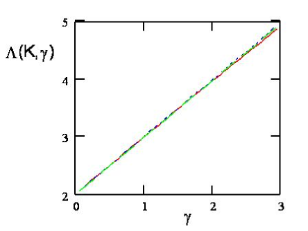
Figure 13: Lagrangian exponent $\Lambda$ vs. Eulerian exponent $\gamma$. The curves for $K=0.1,\ 0.5,\ 0.9$ are all superposed.

We note already here the following very important point: the Lagrangian exponent $\Lambda(\gamma)>2,\ \forall\gamma$. Hence the process described by the V-Langevin equation (93), with the Eulerian velocity correlation (110) in the Corrsin approximation, leads to a diffusive regime for all values of $\gamma>0$ and of $K$. This point will be further discussed below.

We now consider the numerator $h$ of Eq. (110), determined from the logarithmic representation of $\mathcal{L}(\theta)$ (Fig. 12). We first note (Fig. 14) that, for given $K$, it is a very slowly varying function of $\gamma$: we therefore consider it approximately independent of $\gamma$.

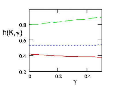
Figure 14: The coefficient $h(K,\gamma)$ vs. the Eulerian exponent $\gamma$, for three values of $K$: $K=0.1$ (solid red), $K=0.3$ (dotted blue), $K=0.5$ (dashed green).

The dependence on $K$ appears to be quadratic, for relatively small values of $K$. It is quite well fitted by the following empiric formula, valid for $\gamma\lesssim 0.5$ (Fig. 15):

$$h(K)\simeq 0.37+1.85~{}K^{2}.$$ (144)

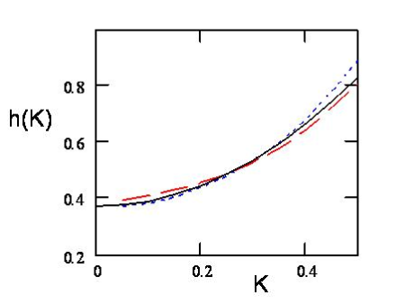
Figure 15: The coefficient $h$ as a function of the Kubo number $K$. Red dashed: $\gamma=0.1$, blue dotted: $\gamma=0.5$. The solid black curve is the empirical fit ( 146).

Finally, the value of the cut-off time is obtained by setting $\mathcal{L}(\theta_{L})=1$.

$$\theta_{L}(\gamma,K)=h(K)^{1/(2+\gamma)}$$ (145)

To sum up, we found a reasonable analytical representation for the Lagrangian velocity correlation in the Corrsin approximation. A simple feature of this representation is the fact that (see Fig. 13 and Fig. 14) each of the two output parameters, $\Lambda,~{}h,$ is a function of a single input parameter $\gamma$ or $K$:

$$\mathcal{L(}\theta)=\left\{\begin{array}[]{c}1,\ \ \ \ \ \ \theta<\theta_{L}(\gamma,K),\\ \dfrac{h(K)}{\theta^{2+\gamma}},\ \ \ \ \ \ \theta>\theta_{L}(\gamma,K)\end{array}\right.~{}\ ,$$ (146)

combined with Eqs. (144) and (145). This analytic approximation is compared to the ”exact” (numerical) Lagrangian velocity correlation in Fig. 16.

Figure 16: ”Exact” numerical Lagrangian velocity correlation (solid red) compared to the analytical approximation (146) (dashed black).

11 Running Diffusion Coefficient

The running diffusion coefficient for an input algebraic Eulerian correlation is obtained from Eq. (108). Using the algebraic form (111) this integral was calculated analytically in Eqs. (110) and (114). Using also the forms (143) - (145) we obtain the result plotted in Fig. 17 for fixed $K=0.3$ and three values of $\gamma=0.1,0.3,0.5$. As we know that the regime is always diffusive, the running diffusion coefficient tends toward a finite positive diffusion constant for sufficiently large times (in practice, $\theta\gtrsim 10$). One sees that the asymptotic diffusion coefficient is a weakly decreasing function of the Eulerian exponent.

Figure 17: Running diffusion coefficient $\mathcal{D}(\theta)$ for three values of $\gamma=0.1$ (solid red), $\gamma=0.3$ (dotted blue), $\gamma=0.5$ (dashed black). $K=0.3.$

Fig. 18 shows the dependence of the diffusion coefficient on the Kubo number for fixed $\gamma=0.1$. The asymptotic diffusion coefficient is a rather strongly increasing function of $K$.

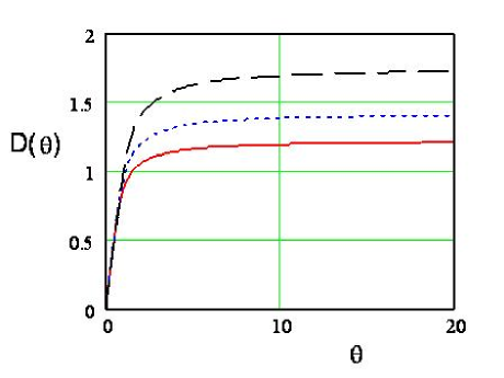
Figure 18: Running diffusion coefficient $\mathcal{D}(\theta)$ for three values of $K=0.1$ (solid red), $K=0.3$ (dotted blue), $K=0.5$ (dashed black). $\gamma=0.1.$

In most existing works on the Langevin equation the Eulerian velocity time-correlation is assumed to decay exponentially ($\beta=1$). This produces a Lagrangian correlation that also has an exponential asymptotic behavior, and thus automatically ensures the convergence of the integral (108) defining the diffusion constant. It is interesting to compare the diffusion coefficients obtained in the algebraic case and in the exponential case. For the latter we use a Eulerian correlation that is tailored in such a way as to resemble the algebraic one: we thus start the exponential decay at the cut-off time of the algebraic one (Fig. 19):

$$\mathcal{T}_{\exp}(\theta/K)=\left\{\begin{array}[]{c}1,\ \ \ \ \theta\leq K\\ \exp\left[\dfrac{\theta-K}{K}\right],\ \ \ \ \ \theta>K\end{array}\right..$$ (147)

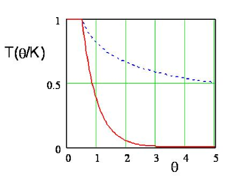
Figure 19: Temporal part of the Eulerian velocity correlation. Solid red: exponential, Eq. (147); dotted blue: algebraic, Eq. (109). $K=0.5,\ \gamma=0.3.$

The Lagrangian velocity correlation is calculated in the Corrsin approximation up to the second iteration, by following exactly the same steps as in Secs. 9 and 10. The result is shown in Fig. 20. (Note that $\mathcal{L}_{\exp}(0)=1$, hence it is not necessary to introduce a cut-off time $\theta_{L}$ as for the algebraic case). As expected, $\mathcal{L}_{\exp}(\theta)$ decays much more quickly: it has no long-time tail as the algebraic one.

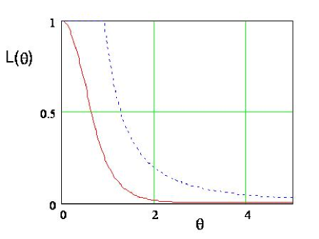
Figure 20: Lagrangian velocity correlation for the case of an algebraic (solid red) [$K=0.5,\ \gamma=0.1$] and of an exponential (dotted blue) Eulerian correlation with the same $K$.

The running diffusion coefficients corresponding to the same parameters are compared in Fig. 21. The algebraic correlation produces a running diffusion coefficient that saturates at a longer time. As a result, the asymptotic diffusion constant $\mathcal{D>D}_{\exp}.$ This results from the fact that the area under the Lagrangian correlation is larger in the algebraic case (Fig. 20), due to the slow decay of the correlation.

Figure 21: Running diffusion coefficient for the case of an algebraic (solid red) [$K=0.5,\ \gamma=0.1$] and of an exponential (dotted blue) Eulerian correlation with the same $K$.

12 Conclusions

Our main purpose in the present work was to study the relation between a ”semi-dynamical” description of a system of particles, based on the V-Langevin equation and its associated hybrid kinetic equation, and on the other hand on a purely stochastic description in terms of a continuous time random walk and its limiting form as a fractional diffusion equation. We wanted, in particular, to find out under what conditions on the velocity correlation function a V-Langevin equation describes a ”strange transport regime”, which could be equivalently represented by a CTRW or a FDE.

It was known from previous work [2] that a subdiffusive regime can appear in some limiting cases. This occurs, e.g., for a collisional plasma in a strong magnetic field, in the limit of infinite correlation length perpendicular to $\mathbf{B}$ [25], [26] or for electrostatic drift wave turbulence in the limit of infinite Kubo number [2]. In these cases, subdiffusion is produced by sticking of the particles to the magnetic field lines, or by their trapping in the turbulent field. It might be stressed that in the latter case, a diffusive or a subdiffusive ($K\rightarrow\infty)$ regime was found even when the spatial correlation is long-range (Lorentzian), but the time correlation is exponential [27]. A superdiffusive regime is, however, much more elusive. To the best of our knowledge, a V-Langevin equation producing Lévy-type superdiffusion was only found for a one-dimensional two-state model (velocity = $\pm V$) [14]. The restriction to a velocity constant in absolute value was necessary in order to replace the Lévy flight CTRW by a Lévy walk.

In the present work we showed that, for one-dimensional systems, the results of [14] concerning the time-fractional superdiffusion can be extended to the more physical case of a general random time-dependent velocity function equipped with an algebraic time-correlation function (but with a Gaussian space-correlation). We confirm that in this case we find a process that is an ”intermediate” between diffusion and wave propagation. This type of superdiffusive processes, distinct from the Lévy-type, has been studied in detail in [9] and [10].

We then generalized our investigation to the study of a random velocity field in two dimensions. In this case one is faced with the difficult problem of determining the Lagrangian velocity correlation, a problem that was treated within the Corrsin approximation. It was first shown that if the Eulerian correlation decays algebraically as $\theta^{-\gamma}$ for long times (and its spatial part is Gaussian), the Lagrangian correlation has the same property, with a different exponent: $\theta^{-\Lambda}$.

We then established a general criterion for the existence of a superdiffusive regime, based on the value of the Lagrangian exponent $\Lambda$. It was shown in Sec. 8 that whenever $0<\Lambda<1$, the regime is superdiffusive and can be equivalently described by a time-fractional FDE. When $\Lambda>1$, however, the semi-dynamical description predicts a diffusive regime for all $\Lambda$, whereas the formally associated FDE predicts subdiffusion, or even looses meaning, for $\Lambda>2$. Thus, the purely stochastic CTRW or FDE descriptions of the turbulence are severely limited in this case by the existence of a bifurcation at $\Lambda=1$.

In the final stage (Sec. 10) the Lagrangian exponent $\Lambda$ was determined numerically. The result shows that $\Lambda=2+\gamma>2$, for all values of $\gamma$ and of $K$. Thus, for the present model and with the approximations used in its treatment: [local approximation of the non-Markovian diffusion equation (54), Corrsin approximation of the Lagrangian velocity correlation (101)]:

• The regime is always normal diffusive, for all values of the input Eulerian parameters $\gamma$ and $K$. There never appears any superdiffusion, in spite of the long algebraic tail of the temporal velocity correlation. This is to be contrasted with the one-dimensional case of a purely time-dependent velocity, where the regime is superdiffusive for all values $0<\gamma<1$.

• The ”formally associated” fractional differential equation, has no meaning. The evolution cannot be described by a purely stochastic process.

• Although the regime is diffusive, the density profile is not a Gaussian packet. Indeed, although the Lagrangian correlation decays sufficiently fast in order to ensure the existence of a finite asymptotic diffusion constant, the non-Markovian character of the equation (107) cannot be neglected for finite time.

The results obtained here may appear somewhat disappointing, in the sense that no time-fractional superdiffusion was found for two-dimensional motion. Nevertheless, we believe that the result of the exhaustive analysis performed here is interesting in exhibiting the limits of a purely stochastic description. It shows that a long-tailed algebraic temporal correlation is not sufficient for producing superdiffusion (for dimensionality $d>1$). In order to obtain a Lévy-type superdiffusive regime, we must presumably act on the spatial part of the Eulerian velocity correlation. This problem is, however, highly non-trivial. On one hand, in the Corrsin approximation, Eq. (106) is invalid, because it is based on the Gaussian form of the spatial Eulerian correlation. But one should go back even further in the chain of approximations. The local approximation leading from Eq. (54) to (55) (in two dimensions) is questionable in the presence of long-range spatial correlations. We hope to come back to this problem in forthcoming work.

Appendix: A Primer on Fractional Calculus

Fractional Calculus has been known to mathematicians for a very long time. The problem appears to have been first raised by L’Hospital and by Leibniz in 1695. The first systematic construction appears in the early 19-th century and is due to Liouville (1832) (well known to every physicist from the first lecture in statistical mechanics), who used this concept in potential theory. It was further developed by B. Riemann in 1847. For a long time the concept was studied only by mathematicians. It entered physics only in the last half of the 20-th century, through the theory of stochastic equations associated with the problems of random walks (Sec. 2).

The search for a natural generalization of the ordinary derivative $d^{n}/dx^{n}$, with $n$: an integer, is clearly attractive for a mathematician. It is as natural as the passage from the integers to rational, and later to real numbers. We must find a way to interpolate in a consistent way the concept of differentiation between two successive integers, $n$ and $n+1$. The way of doing this is however not obvious. Indeed, several different approaches have been devised by mathematicians. We shall only discuss here the one which is most widely used in the literature (for a discussion of other approaches, see [7], [28] and [11]). One will find detailed expositions of the subject in [8], [13], [7], [29], [5], [6], [30]. Excellent tutorials are the papers by [23] and especially [9], [10]. A brief, but very clear summary is given in [16].

The names of fractional integral, fractional derivative, fractional calculus are actually rather improper. The object of these concepts is to extend the notions of integration and of differentiation from integer order $n$ to arbitrary real order $\beta$, not necessarily a fraction. The name has, however, acquired general practice.

RIEMANN-LIOUVILLE FRACTIONAL INTEGRAL

Consider first the multiple integral of order $n$ ($n$: integer) of a real-valued function $f(x)$ of the real variable $x$:

$${}_{a}J_{x}^{n}~{}f(x)=\int_{a}^{x}dx_{1}\int_{a}^{x_{1}}dx_{2}...\int_{a}^{x_{n-1}}dx_{n}~{}f(x_{n}).$$ (148)

The two lower subscripts relate to the limits of integration ($a$ is a fixed real number); the superscript $n$ denotes the order (multiplicity). This equation can be written in the following equivalent form, in terms of a single integral:

$${}_{a}J_{x}^{n}~{}f(x)=\frac{1}{(n-1)!}\int_{a}^{x}dy~{}\frac{f(y)}{(x-y)^{1-n}}.$$ (149)

The equivalence between the two forms is easily demonstrated by partial integration. We may put  ${}_{a}J_{x}^{0}~{}f(x)=f(x)$ [7]. For $n=1$, the formula reduces to the single integration:

$${}_{a}J_{x}^{1}~{}f(x)=\int_{a}^{x}dy~{}f(y)$$ (150)

Let us check $n=2$:

$${}_{a}J_{x}^{2}~{}f(x) = \int_{a}^{x}dy~{}(x-y)~{}f(y)$$

$$= \left.\left\{(x-y)\int_{a}^{y}dx_{1}f(x_{1})\right\}\right|_{a}^{x}-\int_{a}^{x}(-1)\text{ }dy\int_{a}^{y}dx_{2}f(x_{2})$$

$$= \int_{a}^{x}dx_{1}\int_{a}^{x_{1}}dx_{2}~{}f(x_{2}).$$

In the form (149) the way toward a generalization of the operation of integration (149) is obvious:

$$\begin{array}[]{l}{}_{a}J_{x}^{\alpha}f(x)~{}{\large=~{}}\dfrac{1}{\Gamma(\alpha)}{\large~{}}\int_{a}^{x}{\normalsize dy~{}}\dfrac{f(y)}{(x-y)^{1-\alpha}}{\normalsize,\ \ \ \ \alpha>0}:\text{any positive real number.}\end{array}$$ (151)

This is the definition of the Riemann - Liouville (RL) fractional integral of $f(x)$ of arbitrary real order $\alpha$.

Some of the more important properties are given here:

A) RL fractional integral of a monomial

$$\begin{array}[]{l}{}_{0}J_{x}^{\alpha}~{}x^{\mu}{\normalsize=}\dfrac{\Gamma(\mu+1)}{\Gamma(\mu+\alpha+1)}{\normalsize~{}x}^{\mu+\alpha}{\normalsize.}\end{array}$$ (152)

B) Commutative composition rule:

$$\begin{array}[]{l}{}_{0}J_{x}^{\mu}\cdot~{}_{0}J_{x}^{\nu}\cdot f(x)=~{}_{0}J_{x}^{\nu}\cdot~{}_{0}J_{x}^{\mu}\cdot f(x)=~{}_{0}J_{x}^{\mu+\nu}\cdot f(x)\end{array}$$ (153)

Proof:

$${}_{0}J_{x}^{\mu}\cdot~{}_{0}J_{x}^{\nu}\cdot f(x) = \frac{1}{\Gamma(\mu)}\int_{0}^{x}d\xi~{}(x-\xi)^{-1+\mu}~{}\frac{1}{\Gamma(\nu)}\int_{0}^{\xi}d\tau~{}(\xi-\tau)^{-1+\nu}f(\tau)$$

$$= \frac{1}{\Gamma(\mu)\Gamma(\nu)}\int_{0}^{x}d\tau~{}f(\tau)\int_{\tau}^{x}d\xi~{}(x-\xi)^{-1+\mu}(\xi-\tau)^{-1+\nu}$$

Substitute:  $\xi=\tau+(x-\tau)\zeta$

$$= \frac{1}{\Gamma(\mu)\Gamma(\nu)}\int_{0}^{x}d\tau~{}f(\tau)\int_{0}^{1}d\zeta~{}(x-\tau)~{}[\zeta(x-\tau)]^{-1+\nu}~{}[(1+\zeta)(x-\tau)]^{-1+\mu}$$

$$= \frac{1}{\Gamma(\mu)\Gamma(\nu)}\int_{0}^{x}d\tau~{}f(\tau)~{}(x-\tau)^{-1+\mu+\nu}~{}\int_{0}^{1}d\zeta~{}\zeta^{-1+\nu}~{}(1+\zeta)^{-1+\mu}$$

The $\zeta$-integral is well-known is expressed in terms of the well-known $B$-function:

$$\int_{0}^{1}d\tau~{}\tau^{z-1}~{}(1-\tau)^{w-1}=B(z,w)=\frac{\Gamma(z)\Gamma(w)}{\Gamma(z+w)}.$$ (154)

hence:

$${}_{0}J_{x}^{\mu}\cdot~{}_{0}J_{x}^{\nu}\cdot f(x)=\frac{1}{\Gamma(\mu+\nu)}\int_{0}^{x}d\tau~{}(x-\tau)^{-1+\mu+\nu}~{}f(\tau)$$

$$=~{}_{0}J_{x}^{\mu+\nu}f(x)=~{}_{0}J_{x}^{\nu}\cdot~{}_{0}J_{x}^{\mu}\cdot f(x),\ \ \ \ \ QED$$

RIEMANN-LIOUVILLE FRACTIONAL DERIVATIVE

The fractional derivative is constructed by combining the operations of the usual (integer-order) derivative with the fractional integral.

We define the fractional derivative as follows:

$${}_{a}D_{x}^{\alpha}~{}f(x)=\frac{d^{m}}{dx^{m}}\left[{}_{a}J_{x}^{(m-\alpha)}f(x)\right],\ \ \ \alpha>0,\ \ \ \ m-1<\alpha\leq m.$$ (155)

where $\alpha$ is any positive real number, not an integer, and $m$ is the smallest integer larger than $\alpha$.

In order to ”understand intuitively” this rather unusual definition, we may think, very casually, and without any rigour, as follows. We have a solid reference point, viz. a rigorously defined fractional object, the RL integral. We then start with a RL integral of order $m-\alpha$, where $m$ is the smallest integer which makes $m-\alpha>0$, thus ensuring that ${}_{a}J_{x}^{(m-\alpha)}f(x)$ is a true fractional integral (151). Next, we ”differentiate away” the integer $m$, by taking the $m$-th ordinary derivative of this object. This looks like ”lowering the order” of ${}_{a}J_{x}^{(m-\alpha)},$ thus ”transforming” it into ${}_{a}J_{x}^{-\alpha}$, which could be viewed as a fractional integral of negative order, $-\alpha$, to be interpreted as a fractional derivative of order $+\alpha$. But, again, this paragraph is just cavalier talk; in particular, viewing $J^{-\alpha}$ as an ”inverse” to $D^{\alpha}$ is an ambiguous statement, as will be shown below. We now go back to business, and consider Eq. (155) as a given definition, and study some of its consequences.

A basic requirement is that the definition (155) be compatible with the ordinary (integer-order) derivative. When $\alpha$ is an integer, $\alpha=N$, we have $m-1=\alpha=N,$ thus $m=N+1$, and recalling Eq. (150), we have:

$${}_{a}D_{x}^{N}f(x)=\frac{d^{N+1}}{dx^{N+1}}\left[{}_{a}J_{x}^{1}f(x)\right]=\frac{d^{N}}{dx^{N}}~{}\frac{d}{dx}~{}\int_{a}^{x}dy~{}f(y)=\frac{d^{N}}{dx^{N}}~{}f(x);$$

the operation thus reduces to the ordinary differentiation, as it should.

Combining Eqs. (151) and (155) we find:

$$\begin{array}[]{l}{}_{a}D_{x}^{\alpha}f(x)=\dfrac{d^{m}}{dx^{m}}~{}\dfrac{1}{\Gamma(m-\alpha)}~{}\int_{a}^{x}dy~{}\dfrac{f(y)}{(x-y)^{\alpha+1-m}},\ \ \ \alpha>0,\ \ \ \ \ m-1\leq\alpha<m.\end{array}$$ (156)

This is the definition of the Riemann - Liouville (RL) left-fractional derivative of order $\alpha$.

We may also define a Riemann-Liouville (RL) right-fractional derivative in which it is the upper integration limit $b$ that is fixed:

$${}_{x}D_{b}^{\alpha}\phi=\frac{d^{m}}{dx^{m}}~{}\frac{(-1)^{m}}{\Gamma(m-\alpha)}~{}\int_{x}^{b}dy~{}\frac{\phi(y)}{(y-x)^{\alpha+1-m}},\ \ \ \ \ \alpha>0,\ \ \ \ \ \ m-1\leq\alpha<m.$$ (157)

We now explore a few properties of the fractional derivatives: we shall meet some surprises. These are all due to a fundamental fact. The fractional derivative (for any of the forms defined above) of a function $f(x)$ is expressed as an integral of $f(x)$ over a given range of $x$  It is therefore an intrinsically non-local operator. In other words, the value of the fractional derivative (for non-integer $\alpha$) ${}_{a}D_{x}^{\alpha}f(x)$ at the point $x$ depends on the values of $f$ taken in the whole range of integration defining this quantity. It is quite surprising that, upon varying continuously the order $\alpha$, this non-local character disappears suddenly whenever $\alpha$ reaches any integer value! What is not surprising, therefore, is that fractional calculus entered physics when researchers began to be interested in evolutionary processes endowed with memory (”non-Markovian processes”) or in the influence of the spatial neighborhood in the phenomena at a given point $(x,t)$.

a) Linearity:

$${}_{0}D_{x}^{\alpha}~{}[\lambda~{}f(x)+\mu~{}g(x)]=\lambda~{}_{0}D_{x}^{\alpha}~{}f(x)+\mu~{}_{0}D_{x}^{\alpha}g(x)$$ (158)

The proof follows trivially from the definition of the RL derivative.

b) RL Fractional derivative of a monomial:

$$\begin{array}[]{l}{}_{0}D_{x}^{\alpha}~{}x^{\mu}=\dfrac{\Gamma(\mu+1)}{\Gamma(\mu-\alpha+1)}~{}x^{\mu-\alpha},\ \ \ \ \alpha>0,\ \ \ \ \ \mu>-1.\end{array}$$ (159)

Proof.  Using the definition (156):

$${}_{0}D_{x}^{\alpha}~{}x^{\mu}=\frac{d^{m}}{dx^{m}}~{}\frac{1}{\Gamma(m-\alpha)}~{}\int_{0}^{x}dy~{}y^{\mu}~{}(x-y)^{-1+m-\alpha}.$$ (160)

Let us do this calculation in some detail. Substituting $y\rightarrow xt$ we find

$${}_{0}D_{x}^{\alpha}~{}x^{\mu}=\left(\frac{d^{m}}{dx^{m}}~{}x^{m+\mu-\alpha}\right)~{}\frac{1}{\Gamma(m-\alpha)}\int_{0}^{1}dt~{}t^{\mu}~{}(1-t)^{-1+m-\alpha}.$$

The integral appearing here is expressed in terms of the $B$-function, (154), hence:

$${}_{0}D_{x}^{\alpha}~{}x^{\mu}=\left(\frac{\partial^{m}}{\partial x^{m}}~{}x^{m+\mu-\alpha}\right)~{}\frac{1}{\Gamma(m-\alpha)}~{}\frac{\Gamma(m-\alpha)\Gamma(\mu+1)}{\Gamma(\mu+1-\alpha+1)}.$$

Next, we calculate (setting $\gamma=\mu-\alpha)$

$$\frac{d^{m}}{dx^{m}}~{}x^{m+\gamma}=(m+\gamma)(m-1+\gamma)...(1+\gamma)~{}x^{\gamma}.$$

Noting the identity:

$$\Gamma(m+\gamma+1)=(m+\gamma)(m-1+\gamma)...(1+\gamma)~{}\Gamma((1+\gamma),$$

we combine all these partial results to obtain the final formula (159).

The limitation to $\mu>-1$ in Eq. (159) is due to the factor $\Gamma(1+\mu)$ which has a pole in $\mu=-1$. Note that for any non-integer value of $\alpha$ the RL derivative ${}_{0}D_{x}^{\alpha}~{}x^{\mu}$ has a single zero (for any $x\neq 0)$ in the allowed region, namely for $\mu=\alpha-1$ (see below). Indeed, any zero of the right hand side of Eq. (159) originates from the factor $1/\Gamma(\mu+1-\alpha)$ which vanishes whenever its argument is zero or a negative integer, see Fig. 22; a single one of them is larger than $-1$.

$${}_{0}D_{x}^{\alpha}~{}x^{\alpha-1}=0,\ \ \ \ \ \forall\alpha>0.$$ (161)

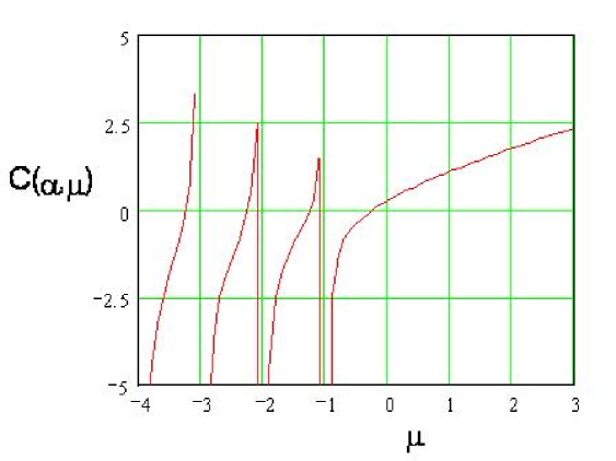
Figure 22: Coefficient $C(\alpha,\mu)=\Gamma(\mu+1)/\Gamma(-\alpha+\mu+1)$ of the RL derivative of $x^{\mu}$ as a function of $\mu.\ \alpha=0.75.$

The formula (159) is deceptively simple, and would correspond with intuition. Just as the ordinary integral-order derivative ($d^{n}/dx^{n})x^{m}$ lowers the power of $x$ by $n$, the fractional derivative transforms $x^{\mu}$ into $x^{\mu-\alpha}$, with a prefactor. But a further reflection shows us that this result is not as innocent as it appears.

b1) RL Fractional derivative of a constant: Consider, indeed, the case $\mu=0$, i.e., the

$${}_{0}D_{x}^{\alpha}~{}cx^{0}=c~{}\frac{\Gamma(1)}{\Gamma(1-\alpha)}~{}x^{-\alpha},$$

i.e.,

$${}_{0}D_{x}^{\alpha}~{}c=\frac{c}{\Gamma(1-\alpha)}~{}x^{-\alpha}\neq 0\$$ (162)

Thus, the RL fractional derivative of non-integer order $\alpha>0$ of a constant is non-zero! Is this result consistent with the ordinary derivative? The answer comes from the properties of the gamma function. Indeed, whenever $\alpha=n$, where $n$ is a non-zero integer, $n=1,2,3,...$ the argument of the $\Gamma$ function is a negative integer, or zero. But we know that

$$\Gamma(0)=\Gamma(-1)=\Gamma(-2)=...=\infty$$

Hence, for any integer value of $\alpha$, Eq. (162) reduces, as it should, to:

$${}_{0}D_{x}^{n}~{}c=0,\ \ \ \ \ n=1,2,...$$ (163)

Another feature of Eq. (159) seems to contradict our previous statement: ${}_{0}D_{x}^{\alpha}~{}x^{\mu}$ is a perfectly local expression, depending only on the value of $x^{\mu}$ at $x$. In order to understand what happens here, we consider the RL derivative of $x^{\mu}$ for a lower integration limit $0<a<x$ instead of zero. Starting the calculation as above, we find after the first step:

$${}_{a}D_{x}^{\alpha}~{}x^{\mu}=\frac{d^{m}}{dx^{m}}\left(~{}x^{m+\mu-\alpha}~{}\frac{1}{\Gamma(m-\alpha)}\int_{a/x}^{1}d\xi~{}\xi^{\mu}~{}(1-\xi)^{-1+m-\alpha}\right),\ \ \ x>a.$$ (164)

There are two important differences with Eq. (160). First, the integral depends on $x$, through its lower limit; hence, the $m$-th derivative acts on the whole product, thus yielding a much more complicated $x$-dependence. Next, the integral with a non-zero lower limit is no longer a $B$-function, but rather a very complicated hypergeometric function. In order to illustrate our case, we consider the simplest non-trivial case that leads to simple calculations: $\mu=2$, $\alpha=\frac{1}{2}$, hence $m=1$. Eq. (164) then reduces to:

$${}_{a}D_{x}^{1/2}~{}x^{2}=\frac{d}{dx}\left(~{}x^{5/2}~{}\frac{1}{\Gamma(1/2)}\int_{a/x}^{1}d\xi~{}\xi^{2}~{}(1-\xi)^{-1/2}\right).$$ (165)

The integral is tabulated; a simple calculation then leads to the result:

$${}_{a}D_{x}^{1/2}~{}x^{2}=\frac{1}{\sqrt{\pi}}\left[\frac{x^{2}}{\sqrt{x-a}}+2x\sqrt{x-a}-\frac{(x-a)^{3/2}}{3}\right],\ \ \ x>a.$$ (166)

The result reduces to Eq. (159) when $a\rightarrow 0$:

$${}_{0}D_{x}^{1/2}~{}x^{2}=\frac{8}{3\sqrt{\pi}}~{}x^{3/2}=\frac{\Gamma(3)}{\Gamma(5/2)}~{}x^{3/2}.$$ (167)

The non-local character of the fractional derivative is now luminously illustrated. The complicated function appearing in the right hand side of Eq. (166) is determined by the choice of the function $\xi^{\mu}$ in Eq. (164), hence by its values taken over the whole integration range. In particular, the fractional derivative depends explicitly on the lower integration limit $a$. A striking fact is the singularity of the RL fractional derivative when $x\rightarrow a$. This singularity is present for any $a$, arbitrarily close to zero, but disappears when $a=0$. When $x\gg a$, ${}_{a}D_{x}^{1/2}~{}x^{2}\rightarrow~{}_{0}D_{x}^{1/2}~{}x^{2}$. All this clearly shows that the value $a=0$ is not a generic one. The situation is illustrated in Fig. 23.

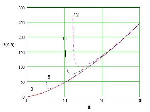
Figure 23: Fractional derivative of $x^{2}$:  ${}_{a}D_{x}^{1/2}x^{2}\equiv D(x,a)$, for $a=0,5,10,12$.

c)Inversion of the RL fractional derivative.

Many authors state rather loosely that ”the RL fractional derivative is the inverse of the RL fractional integral”. They even adopt the notation:  ${}_{a}J_{x}^{\alpha}\equiv~{}_{a}D_{x}^{-\alpha}$ [7]. It will be shown now that this statement is, for the least, ambiguous. Hence Podlubny’s notation should preferably be avoided in order to avoid misunderstandings (Mainardi).

c1) RL Fractional derivative of a fractional integral of same order.

$$\begin{array}[]{l}{}_{0}D_{x}^{\alpha}~{}[_{0}J_{x}^{\alpha}~{}f(x)]=f(x).\end{array}$$ (168)

Proof:

For integer $\alpha=n\geq 1$:

$${}_{0}D_{x}^{n}~{}[_{0}J_{x}^{n}~{}f(x)] = \frac{d^{n}}{dx^{n}}~{}\frac{1}{(n-1)!}~{}\int_{0}^{x}dy~{}(x-y)^{n-1}f(y)$$

$$= \frac{d}{dx}~{}\int_{0}^{x}dy~{}f(y)=f(x)$$

For non-integer $\alpha$, we enclose this number again between its nearest neighbor integers, defining the integer $k$ as: $k-1\leq\alpha<k.$

Using now the composition rule (153) for the fractional integrals, we note the identity:

$${}_{0}J_{x}^{k-\alpha}\cdot[~{}_{0}J_{x}^{\alpha}~{}f(x)]=~{}_{0}J_{x}^{k}~{}f(x)$$

Using now the definition (155) we have:

$${}_{0}D_{x}^{\alpha}~{}[_{0}J_{x}^{\alpha}~{}f(x)]=\frac{d^{k}}{dx^{k}}~{}\left\{{}_{0}J_{x}^{k-\alpha}~{}[_{0}J_{x}^{\alpha}~{}f(x)]\right\}=\frac{d^{k}}{dx^{k}}~{}_{0}J_{x}^{k}~{}f(x)=f(x).$$

(The result follows from the fact that the last step only involves operations of integer order $k$, i.e., ordinary derivative and integral.

)

From the result (168) one is tempted to conclude that, indeed, ”the RL fractional derivative is the inverse of the RL fractional integral”: the fractional RL derivative annuls the action of the fractional integral. The situation is, however, not so clear-cut. It appears from the following property that the double operation  $D~{}J$ is not commutative! Indeed:

c2) Fractional integral of a RL fractional derivative of the same order.

$$\begin{array}[]{l}{}_{0}J_{x}^{\alpha}~{}[_{0}D_{x}^{\alpha}~{}f(x)]=f(x)-\sum\limits_{j=1}^{k}~{}\left[{}_{0}D_{x}^{\alpha-j}~{}f(x)\right]_{x=0}~{}\dfrac{x^{\alpha-j}}{\Gamma(\alpha-j+1)},\ \ \ \ k-1\leq\alpha<k.\end{array}$$ (169)

Proof.

$${}_{0}J_{x}^{\alpha}~{}\left[{}_{0}D_{x}^{\alpha}~{}f(x)\right]=~{}\frac{1}{\Gamma(\alpha)}~{}\int_{0}^{x}dy~{}(x-y)^{\alpha-1}~{}_{0}D_{y}^{\alpha}~{}f(y)$$

$$=\frac{1}{\Gamma(\alpha)}~{}\int_{0}^{x}dy~{}\frac{1}{\alpha}~{}\left[\frac{d}{dx}(x-y)^{\alpha}\right]~{}_{0}D_{y}^{\alpha}~{}f(y)$$

$$=\frac{d}{dx}~{}\left\{\frac{1}{\Gamma(\alpha+1)}~{}\int_{0}^{x}dy~{}(x-y)^{\alpha}~{}_{0}D_{y}^{\alpha}~{}f(y)\right\}$$

$$=\frac{d}{dx}~{}\left\{\frac{1}{\Gamma(\alpha+1)}~{}\int_{0}^{x}dy~{}(x-y)^{\alpha}~{}\frac{d^{k}}{dy^{k}}~{}_{0}J_{y}^{k-\alpha}~{}f(y)\right\}.~{}$$

A partial integration yields:

$$= \frac{d}{dx}\left\{\frac{1}{\Gamma(\alpha)}\int_{0}^{x}dy~{}(x-y)^{\alpha-1}~{}\frac{d^{k-1}}{dy^{k-1}}~{}_{0}J_{y}^{k-\alpha}~{}f(y)\right.$$

$$\left.-\frac{1}{\Gamma(\alpha+1)}~{}x^{\alpha}~{}\left[\frac{d^{k-1}}{dx^{k-1}}~{}_{0}J_{x}^{k-\alpha}f(x)\right]_{x=0}\right\}.~{}$$

Continuing the partial integrations, and using Eqs. (151) and (153), we end up with:

$$=\frac{d}{dx}\left\{\frac{1}{\Gamma(\alpha-k+1)}~{}\int_{0}^{x}dy~{}(x-y)^{\alpha-k}~{}_{0}J_{y}^{k-\alpha}~{}f(y)\right.$$

$$\left.-\sum\limits_{j=1}^{k}\left[\frac{d^{k-j}}{dx^{k-j}}~{}_{0}J_{x}^{k-\alpha}f(x)\right]_{x=0}~{}\frac{x^{\alpha-j+1}}{\Gamma(\alpha-j+2)}\right\}$$

$$=\frac{d}{dx}\left\{~{}_{0}J_{x}^{\alpha-k+1}\cdot~{}_{0}J_{x}^{k-\alpha}f(x)\right.$$

$$\left.-\sum\limits_{j=1}^{k}\left[\frac{d^{k-j}}{dx^{k-j}}~{}_{0}J_{x}^{k-\alpha}f(x)\right]_{x=0}~{}\frac{x^{\alpha-j+1}}{\Gamma(\alpha-j+2)}\right\}$$

$$=~{}\frac{d}{dx}\left\{{}_{0}J_{x}^{1}f(x)-\sum\limits_{j=1}^{k}\left[\frac{d^{k-j}}{dx^{k-j}}~{}_{0}J_{x}^{k-\alpha}f(x)\right]_{x=0}~{}\frac{x^{\alpha-j+1}}{\Gamma(\alpha-j+2)}\right\}$$

$$=f(x)-\sum\limits_{j=1}^{k}\left[\frac{d^{k-j}}{dx^{k-j}}~{}_{0}J_{x}^{k-\alpha}f(x)\right]_{x=0}~{}\frac{x^{\alpha-j}}{\Gamma(\alpha-j+1)},\ \ \ \ QED$$

It is precisely because of this non-commutativity of integration and differentiation that one cannot state unambiguously that one operation is the inverse of the other.

d) General composition rules.

In all subsequent formulae we take the lower limit  $a=0$. We simplify the notations as follows:  ${}_{0}J_{x}^{\alpha}=J^{\alpha},$   ${}_{0}D_{x}^{\alpha}=D^{\alpha}.$ The proofs of the following results are very similar to the previous ones [7].

d1) Composition of two fractional integrals.  [see (153)]

$$\begin{array}[]{c}J^{\alpha}~{}J^{\beta}~{}f(x)=J^{\beta}~{}J^{\alpha}~{}f(x)=J^{\alpha+\beta}~{}f(x)\end{array}$$ (170)

d2) RL derivative of fractional integral.

$$\begin{array}[]{c}D^{\alpha}~{}J^{\beta}~{}f(x)=J^{\beta-\alpha}~{}f(x),\ \ \ \ \ \ 0<\alpha<\beta\\ D^{\alpha}~{}J^{\beta}~{}f(x)=D^{\alpha-\beta}~{}f(x),\ \ \ \ \ 0<\beta<\alpha\end{array}$$ (171)

d3) Fractional integral of RL derivative.

$$\begin{array}[]{c}J^{\alpha}~{}D^{\beta}~{}f(x)=D^{\beta-\alpha}~{}f(x)-\sum\limits_{j=1}^{n}~{}\left[D^{\beta-j}~{}f(x)\right]_{x=0}~{}\dfrac{x^{\alpha-j}}{\Gamma(\alpha-j+1)},\\ 0<\alpha<\beta,\ \ \ \ n-1\leq\beta<n\end{array}$$ (172)

$$\begin{array}[]{c}J^{\alpha}~{}D^{\beta}~{}f(x)=J^{\alpha-\beta}~{}f(x)-\sum\limits_{j=1}^{n}~{}\left[D^{\beta-j}~{}f(x)\right]_{x=0}~{}\dfrac{x^{\alpha-j}}{\Gamma(\alpha-j+1)},\\ 0<\beta<\alpha,\ \ \ n-1\leq\beta<n\end{array}$$ (173)

d4) Composition of RL derivatives.

$$\begin{array}[]{l}\begin{array}[]{c}{}_{0}D_{x}^{\alpha}\cdot~{}_{0}D_{x}^{\beta}~{}f(x)=~{}_{0}D_{x}^{\alpha+\beta}~{}f(x)-\sum\limits_{j=1}^{n}\left[~{}_{0}D_{x}^{\beta-j}f(x)\right]_{x=0}~{}\dfrac{x^{-\alpha-j}}{\Gamma(-\alpha-j+1)},\\ {}_{0}D_{x}^{\beta}\cdot~{}_{0}D_{x}^{\alpha}~{}f(x)=~{}_{0}D_{x}^{\alpha+\beta}~{}f(x)-\sum\limits_{j=1}^{m}\left[~{}_{0}D_{x}^{\alpha-j}f(x)\right]_{x=0}~{}\dfrac{x^{-\beta-j}}{\Gamma(-\beta-j+1)}\\ \ m-1\leq\alpha<m,\ \ \ \ n-1\leq\beta<n\end{array}\end{array}$$ (174)

Integral transforms of fractional operators.

A)  Fourier transform

The Fourier transform involves integrals ranging from $-\infty$ to $+\infty$. This implies a number of technical assumptions about the regularity of the functions appearing in the theory: we do not discuss them here, assuming that all conditions are satisfied for the existence of the objects of the forthcoming equations. We begin with the following result:

$$\begin{array}[]{c}{}_{-\infty}D_{x}^{\alpha}~{}e^{ikx}=(ik)^{\alpha}~{}e^{ikx}.\end{array}$$ (175)

Proof:

$$F_{+}(x)\equiv~{}_{-\infty}D_{x}^{\alpha}~{}e^{ikx}=\frac{1}{\Gamma(m-\alpha)}~{}\frac{d^{m}}{dx^{m}}~{}\int_{-\infty}^{x}dy~{}(x-y)^{-1+m-\alpha}~{}e^{iky}$$

$$=\frac{1}{\Gamma(m-\alpha)}~{}\frac{d^{m}}{dx^{m}}~{}e^{ikx}\int_{0}^{\infty}dt~{}t^{-1+m-\alpha}~{}e^{-ikt}$$

$$,\ \ \ \ m-1\leq\alpha<m$$

where we set $x-y=t$. We now note that, from the definition of $m$, we have:  $0<m-\alpha\leq 1$. We may thus use the tabulated integral:

$$\int_{0}^{\infty}d\xi~{}\xi^{\gamma-1}~{}e^{-ik\xi}=(ik)^{-\gamma}~{}\Gamma(\gamma),\ \ \ \ \ 0<\gamma<1$$

Hence:

$${}_{-\infty}D_{x}^{\alpha}~{}e^{ikx} = \frac{1}{\Gamma(m-\alpha)}~{}\frac{d^{m}}{dx^{m}}~{}e^{ikx}~{}(ik)^{-m+\alpha}~{}\Gamma(m-\alpha)$$

$$= (ik)^{\alpha}~{}e^{ikx},\ \ \ \ \ \ \ QED$$

This expression is not very convenient in applications. On one hand, the appearance of $i^{\alpha}$ is somewhat awkward. But more important, if we wish to use this result in relation with the Fourier transform, we need to cover the whole range ($-\infty,\ \infty)$, and not only the left range ($-\infty,\ x$). We therefore consider also the right RL fractional derivative (157):

$$\begin{array}[]{c}{}_{x}D_{\infty}^{\alpha}~{}e^{ikx}=(-ik)^{\alpha}~{}e^{ikx}.\end{array}$$ (176)

Proof:

$$F_{-}(x) \equiv ~{}_{x}D_{\infty}^{\alpha}~{}e^{ikx}=\frac{(-1)^{m}}{\Gamma(m-\alpha)}~{}\frac{d^{m}}{dx^{m}}~{}\int_{x}^{\infty}dy~{}(y-x)^{-1+m-\alpha}~{}e^{iky}$$

$$= \frac{(-1)^{m}}{\Gamma(m-\alpha)}~{}\frac{d^{m}}{dx^{m}}~{}\int_{-\infty}^{-x}d\eta~{}(-\eta-x)^{-1+m-\alpha}~{}e^{-ik\eta}$$

Setting $\xi=-x$, we have:

$$F_{-}(x)=\frac{1}{\Gamma(m-\alpha)}~{}\frac{d^{m}}{d\xi^{m}}~{}\int_{-\infty}^{\xi}d\eta~{}(-\eta+\xi)^{-1+m-\alpha}~{}\left(e^{ik\eta}\right)^{\ast}=F_{+}^{\ast}(\xi)$$

Thus:

$$F_{-}(x)=F_{+}^{\ast}(\xi)=(-ik)^{\alpha}~{}e^{-ik\xi}=(-ik)^{\alpha}~{}e^{ikx}\ \ \ \ \ \ \ \ \ QED$$

In order to adapt the previous results to the Fourier transform, in particular to cover the whole range $(-\infty,~{}+\infty)$, we define a new type of fractional derivative, which is totally symmeric. It is justified by the linearity property of the RL derivative (158):

$$\begin{array}[]{c}D_{|x|}^{\alpha}~{}f(x)=-\dfrac{1}{2~{}\cos\dfrac{\pi\alpha}{2}}~{}\left[~{}_{-\infty}D_{x}^{\alpha}+~{}_{x}D_{\infty}^{\alpha}\right]~{}f(x)\end{array}$$ (177)

This is called the Riesz fractional derivative.

The usefulness of this concept appears obviously in the following result, expressing the Fourier transform of the Riesz derivative:

$$\begin{array}[]{c}\mathcal{F}~{}\left\{D_{|x|}^{\alpha}~{}f(x)\right\}=-|k|^{\alpha}~{}\widehat{f}(k)\end{array}$$ (178)

where  $\widehat{f}(k)$ denotes the Fourier transform of  $f(x)$.

Proof:

$$\mathcal{F}~{}\left\{D_{|x|}^{\alpha}~{}f(x)\right\} = \mathcal{F}~{}\left\{D_{|x|}^{\alpha}~{}\int dk^{\prime}~{}e^{-ik^{\prime}x}~{}\widehat{f}(k^{\prime})\right\}$$

$$= -\mathcal{F~{}}\left\{\int dk^{\prime}~{}|k^{\prime}|^{\alpha}~{}e^{-ik^{\prime}x}~{}\widehat{f}(k^{\prime})\right\}$$

$$= -\frac{1}{2\pi}~{}\int dx~{}e^{ikx}~{}\int dk^{\prime}~{}|k^{\prime}|^{\alpha}~{}e^{-ik^{\prime}x}~{}\widehat{f}(k^{\prime})$$

$$= -~{}|k|^{\alpha}~{}\widehat{f}(k),\ \ \ \ \ QED$$

The result (178) ends our quest of the Fourier transform of the (Riesz) fractional derivative of a function, expressed in terms of the Fourier transform of that function.

B) Laplace transform

The (direct) Laplace transform of a function involves an integral over the variable from $0$ to $\infty.$ It is therefore particularly well adapted to the study of functions of time, when the latter is restricted to positive values. The two properties of the Laplace transform that are most useful in applications (especially for the solution of differential equations are:

The convolution theorem: for any two functions $f(t)$, $g(t)$ of time, defined in the range ($0,\ \infty$), their convolution is defined as:

$$(f\ast g)=\int_{0}^{t}d\tau~{}f(t-\tau)~{}g(\tau)$$ (179)

Laplace transform of the (ordinary) derivative:

$$\mathcal{L~{}}\left\{f^{(n)}(t)\right\}=s^{n}~{}\widetilde{f}(s)-\sum\limits_{j=0}^{n-1}~{}s^{n-j-1}~{}f^{(j)}(0)$$ (180)

where $f^{(n)}(t)$ is the $n$-th time derivative of $f(t)$, and $\widetilde{f}(s)$ is the Laplace transform of $f(t)$. The explicit appearance of the functions $f^{(j)}(0)$ in this formula makes the Laplace transform a particularly useful tool for the solution of initial value problems. We may now note that the value $j=0$ in the sum of the right hand side is ”special”: it corresponds to $f^{(0)}(t)=f(t)$, whereas all other terms in the sum contain true derivatives:

$$\mathcal{L~{}}\left\{f^{(n)}(t)\right\}=s^{n}~{}\widetilde{f}(s)-s^{n-1}~{}f(0)-\sum\limits_{j=1}^{n-1}~{}s^{n-j-1}~{}f^{(j)}(0)$$ (181)

We now consider the Laplace transforms of the various objects of fractional calculus.

a) Laplace transform of the fractional integral.

This is easily obtained by noting that the RL integral can be viewed as a convolution:

$${}_{0}J_{t}^{\beta}~{}f(t)=\frac{1}{\Gamma(\beta)}~{}\int_{0}^{t}d\tau~{}(t-\tau)^{\beta-1}~{}f(\tau)=t^{\beta-1}\ast\frac{1}{\Gamma(\beta)}~{}f(t)~{}$$ (182)

Hence, noting the well-known result:

$$\mathcal{L~{}}(t^{\beta-1})=\Gamma(\beta)~{}s^{-\beta},\ \ \ \ \beta>0,$$ (183)

we find immediately, using the convolution theorem (179):

$$\begin{array}[]{c}\mathcal{L~{}}\left\{~{}_{0}J_{t}^{\beta}~{}f(t)\right\}=s^{-\beta}~{}\widetilde{f}(s).\end{array}$$ (184)

b) Laplace transform of the RL derivative.

We write the RL derivative (155) in the form:

$${}_{0}D_{t}^{\beta}~{}f(t)\equiv\frac{d^{m}}{dt^{m}}~{}g(t),\ \ \ \ m-1\leq\beta<m$$ (185)

with:

$$g(t)=~{}_{0}J_{t}^{m-\beta}~{}f(t)$$ (186)

Using Eq. (180) for the $m$-th (ordinary) derivative, we have:

$$\mathcal{L}~{}\left\{~{}_{0}D_{t}^{\beta}~{}f(t)\right\}=s^{m}~{}\widetilde{g}(s)-\sum\limits_{j=0}^{m-1}~{}s^{j}~{}g^{(m-j-1)}(0)$$ (187)

Next, we calculate:

$$g^{(m-j-1)}=\frac{d^{m-j-1}}{dt^{m-j-1}}~{}\frac{1}{\Gamma(m-\beta)}~{}\int_{0}^{t}d\tau~{}(t-\tau)^{m-\beta-1}~{}f(\tau)~{}$$ (188)

Using Eq. (171), we find:

$$g^{(m-j-1)}=~{}_{0}D_{t}^{m-j-1}~{}_{0}J_{t}^{m-\beta}~{}f(t)=\mathcal{O}^{-\beta+j+1}~{}f(t),$$ (189)

where:

$$\mathcal{O}^{\mu}=\left\{\begin{array}[]{c}{}_{0}J_{t}^{\mu},\ \ \ \ \mu>0\\ {}_{0}D_{t}^{\mu},\ \ \ \ \mu<0\end{array}\right..$$ (190)

From the two constraints: $m-1<\beta<m$ and  $0\leq j\leq m-1$, we deduce:

• when $j=m-1$, we have $-\beta+j+1=m-\beta>0$, hence:  $\mathcal{O}^{\mu}=~{}_{0}J_{t}^{\mu}$ ,

• when $j<m-1$, we have $-\beta+j+1<0$, hence:  $\mathcal{O}^{\mu}=~{}_{0}D_{t}^{\mu}.$

Note also, from Eq. (184):

$$\widetilde{g}(s)=\mathcal{L}~{}\left\{~{}_{0}J_{t}^{-\beta+m}f(t)\right\}=s^{\beta-m}~{}\widetilde{f}(s)$$

We thus obtain the final form of the Laplace transform of the RL fractional derivative:

$$\begin{array}[]{c}\mathcal{L}~{}\left\{~{}_{0}D_{t}^{\beta}~{}f(t)\right\}=s^{\beta}~{}\widetilde{f}(s)-s^{m-1}~{}\left[~{}_{0}J_{t}^{-\beta+m}~{}f(t)\right]_{t=0}-\sum\limits_{j=0}^{m-2}s^{j}~{}\left[~{}_{0}D_{t}^{\beta-j-1}~{}f(t)\right]_{t=0}.\end{array}$$ (191)

The analogy with Eq. (181) is striking. The first term has the same form. In the second term the initial value of the function $f(0)$ is replaced, for non-integer $\beta,$ by the initial value of the fractional integral ${}_{0}J_{t}^{-\beta+m}~{}f(t)$,  whereas in the terms under the sum, the initial values of the ordinary derivatives are replaced by the initial values of the corresponding RL fractional derivatives. In spite of this analogy, the RL time-derivative is not easily adapted to the physical applications. The Laplace transform is well known to be a valuable tool for the solution of initial value problems of differential equations, because it incorporates these initial values in Eq. (181). If we now consider initial value problems of fractional differential equations involving RL fractional derivatives with respect to time, we are faced with a serious difficulty if we try to use a Laplace transformation. The specification of (physical) values of the unknown function and of a sufficient number of its derivatives at $t=0$, this does not allow us to determine the correponding initial valued of the fractional integrals and derivatives appearing in Eq. (191). This difficulty has been overcome by M. Caputo in [31], [32] by introducing an alternative definition of the fractional derivative, that is particularly useful for functions of a variable restricted to a finite range, such as time $\in(0,\ t)$.

The Caputo fractional derivative.

The Caputo fractional derivative is defined as follows:

$$\begin{array}[]{c}{}_{0}^{C}D_{t}^{\beta}~{}f(t)=\dfrac{1}{\Gamma(n-\beta)}~{}\int\nolimits_{0}^{t}d\tau~{}\dfrac{1}{(t-\tau)^{\beta+1-n}}~{}\dfrac{d^{n}}{d\tau^{n}}~{}f(\tau),\ \ \ \ n-1\leq\beta<n.\end{array}$$ (192)

Thus, the only difference with the RL derivative Eq.(156) is the commutation of the integration and the differentiation. The Caputo derivative results from a composition of a fractional integral with an ordinary derivative:

$${}_{0}^{C}D_{t}^{\beta}~{}f(t)=~{}_{0}J_{t}^{n-\beta}~{}\left[\frac{d^{n}}{dt^{n}}~{}f(t)\right]$$ (193)

Let us introduce a simplified notation:

$${}_{0}J_{t}^{\beta}\rightarrow J^{\beta},\ \ \ \ _{0}D_{t}^{\beta}\rightarrow D^{\beta},\ \ \ \ _{0}^{C}D_{t}^{\beta}\rightarrow D_{\ast}^{\beta}$$ (194)

The Caputo derivative is related to the Riemann-Liouville one as follows [8]:

$$\begin{array}[]{c}D_{\ast}^{\beta}~{}f(t)=D^{\beta}~{}f(t)-\sum\limits_{j=0}^{n-1}~{}f^{(j)}(0)~{}\dfrac{t^{j-\beta}}{\Gamma(j-\beta+1)}.\end{array}$$ (195)

We give here the proof for the case $0<\beta<1$, which implies $n=1$. The proof of the general case is similar, but longer.

$$\Gamma(1-\beta)~{}D^{\beta}f(t) = \frac{d}{dt}~{}\int_{0}^{t}d\tau~{}\frac{f(\tau)}{(t-\tau)^{\beta}}=\left.\left[\frac{f(\tau)}{(t-\tau)}\right]\right|_{\tau=t}+\int_{0}^{t}d\tau~{}\left[\frac{d}{dt}~{}(t-\tau)^{-\beta}\right]~{}f(\tau)$$

$$= \left.\left[\frac{f(\tau)}{(t-\tau)}\right]\right|_{\tau=t}-\left.\left[\frac{f(\tau)}{(t-\tau)}\right]\right|_{\tau=0}^{\tau=t}+\int_{0}^{t}d\tau~{}\frac{1}{(t-\tau)^{\beta}}~{}\frac{d}{d\tau}f(\tau)$$

$$= t^{-\beta}~{}f(0)+\int_{0}^{t}d\tau~{}\frac{1}{(t-\tau)^{\beta}}~{}\frac{d}{d\tau}f(\tau);$$

Hence, finally:

$$D_{\ast}^{\beta}~{}f(t)=D^{\beta}~{}f(t)-\frac{1}{\Gamma(1-\beta)}~{}t^{-\beta},\ \ \ \ \ 0<\beta<1$$ (196)

which agrees with Eq. (195).

An important property, which is obvious from Eq. (192), and also from (196), combined with (162), is:

$$D_{\ast}^{\beta}~{}1=0,$$ (197)

which makes the Caputo derivative closer to the ordinary derivative.

We now consider the composition of the Caputo derivative $D_{\ast}^{\beta}$ with the fractional integral of the same order $J^{\beta}$. A first relation is immediately obtained from the combination of Eqs. (168) and (195):

$$\begin{array}[]{c}D_{\ast}^{\beta}~{}J^{\beta}~{}f(t)=f(t)-\sum\limits_{j=1}^{n-1}~{}\left[J^{\beta-j}~{}f(t)\right]_{t=0}~{}\dfrac{t^{j-\beta}}{\Gamma(j-\beta+1)}.\end{array}$$ (198)

Commuting the integral and the derivative and using successively Eqs. (195), (169) and (152) we obtain:

$$J^{\beta}~{}D_{\ast}^{\beta}~{}f(t)=J^{\beta}~{}D^{\beta}~{}f(t)-\sum\limits_{j=0}^{n-1}~{}\frac{1}{\Gamma(j-\beta+1)}~{}\left[\frac{d^{j}}{dt^{j}}~{}f(t)\right]_{t=0}~{}J^{\beta}~{}t^{j-\beta}$$

$$=f(t)-\sum\limits_{k=1}^{n}~{}\left[D^{\beta-k}~{}f(t)\right]_{t=0}~{}\frac{t^{\beta-k}}{\Gamma(\beta-k+1)}-\sum\limits_{j=0}^{n-1}~{}\left[\frac{d^{j}}{dt^{j}}~{}f(t)\right]_{t=0}~{}\frac{t^{j}}{\Gamma(j+1)}$$

and finally (with $k\rightarrow j+1$):

$$\begin{array}[]{c}J^{\beta}~{}D_{\ast}^{\beta}~{}f(t)=f(t)-\sum\limits_{j=0}^{n-1}~{}\left\{\left[D^{\beta-j-1}f(t)\right]_{t=0}~{}\dfrac{t^{\beta-j-1}}{\Gamma(\beta-j)}+f^{(j)}(0)~{}\dfrac{t^{j}}{\Gamma(j+1)}\right\}\end{array}$$ (199)

Eqs. (198) and (199) show that the Caputo derivative is not an inverse of the fractional integral, either to the left or to the right. General composition rules of the type of Eqs. (170) - (174) can be derived for the Caputo derivative, using the previous results; they are rather complicated, and will not be written down explicitly. We now consider the most important property of the Caputo derivative.

Laplace transform of the Caputo derivative.

The result is easily obtained by combining the definition (193) with Eqs. (184) and (181):

$$\mathcal{L}~{}\left[~{}_{0}^{C}D_{t}^{\beta}~{}f(t)\right] = \mathcal{L}~{}\left[~{}_{0}J_{t}^{n-\beta}\left(\frac{d^{n}f(t)}{dt^{n}}\right)\right]=s^{\beta-n}~{}\mathcal{L}~{}\left(\frac{d^{n}f(t)}{dt^{n}}\right)$$

$$= s^{\beta-n}~{}\left[s^{n}~{}\widetilde{f}(s)-s^{n-1}~{}f(0)-\sum\limits_{k=0}^{n-2}~{}s^{j}~{}f^{(n-k-1)}(0)\right],$$

and finally, setting $n-k-1=j$:

$$\begin{array}[]{c}\mathcal{L}~{}\left[~{}_{0}^{C}D_{t}^{\beta}~{}f(t)\right]=s^{\beta}~{}\widetilde{f}(s)-s^{\beta-1}~{}f(0)-\sum\limits_{j=1}^{n-1}~{}s^{\beta-j-1}~{}f^{(j)}(0),\ \ \ \ \ n-1<\beta<n.\end{array}$$ (200)

This result has exactly the same form as the Laplace transform of an ordinary derivative, Eq. (181), with $n\rightarrow\beta$. Contrary to the Laplace transform of the RL derivative (191), the Laplace transform of the Caputo derivative only involves the initial values of the function $f(t)$ and of its ordinary derivatives, instead of the initial values of the fractional integral and of the RL fractional derivatives. In any physical differential equation, the former are the given input. This property makes the Caputo derivative an invaluable tool for solving initial value problems of fractional differential equations.

References

- [1] J. Klafter and I.M. Sokolov, Anomalous diffusion spreads its wings, Phys. World, August 2005, p. 29-32
- [2] R. Balescu, Aspects of Anomalous Transport in Plasmas, IoP (Taylor & Francis), London, 2005
- [3] E.W. Montroll and G.H. Weiss, Random walks on lattices, II, J. Math. Phys., 6, 167-181, 1965.
- [4] E.W. Montroll and M.F. Shlesinger, On the wonderful world of random walks, in: Studies of Statistical Mechanics (edited by J.L. Lebowitz and E.W. Montroll), vol. 11, p.5-121, North Holland, Amsterdam, 1984.
- [5] R. Metzler and J. Klafter, The random walk’s guide to anomalous diffusion: a fractional dynamics approach, Phys. Reports, 339, 1-77, 2000
- [6] R. Metzler and J. Klafter, The restaurant at the end of the random walk: recent developments in the description of anomalous transport by fractional dynamics, J. Phys. A: Math. Gen., 37, R161-R208, 2004.
- [7] I. Podlubny, Fractional Differential Equations, Acad. Press, New York, 1999
- [8] R. Gorenflo and F. Mainardi, Fractional calculus, integral and differential equations of fractional order, in: Fractals and Fractional Calculus in Continuum Mechanics (edited by A. Carpinteri and F. Mainardi), p. 223-276, Springer, Wien, 1997
- [9] F. Mainardi, Yu. Luchko and G. Pagnini, The fundamental solution of the space-time fractional diffusion equation, Fract. Calc. Appl. Analysis, 4, 153-192, 2001. Available from http://www.fracalmo.org
- [10] F. Mainardi and G. Pagnini, The Wright functions as solutions of the time-fractional diffusion equation, Appl. Math. Comput., 141, 51-62, 2003. Available from http://www.fracalmo.org
- [11] B.J. West, M. Bologna and P. Grigolini, Physics of Fractal Operators, Springer, New York, 2003
- [12] P. Grigolini, The Continuous Random Walk versus the Generalized Master Equation, Adv. Chem. Phys. 113, 357-474, 2006.
- [13] R. Gorenflo and F. Mainardi, Simply and multiply scaled diffusion limits for continuous time random walks, J. Phys., Conference Series, 7, 1-16, 2005
- [14] B.J. West, P. Grigolini, R. Metzler and T. Nonnenmacher, Fractional diffusion and Lévy stable processes, Phys. Rev. E 55, 99-106, 1997
- [15] B. Ph. van Milligen, R. Sanchez and B.A. Carreras, Probabilistic finite-size transport models for fusion: Anomalous transport and scaling laws, Phys. Plasmas, 11, 2272-2285, 2004
- [16] D. del-Castillo Negrete, B.A. Carreras and V.E. Lynch, Fractional diffusion in plasma turbulence, Phys. Plasmas, 11, 3854-3864, 2004
- [17] R.C. Ball, S. Havlin and G.H. Weiss, Non-Gaussian random walks, J. Phys. A 20, 4055-4059, 1987
- [18] J.P. Bouchaud and A. Georges, Anomalous diffusion in disordered systems : statistical mechanisms, models and physical applications, Phys. Rep., 195, 127-293, 1990
- [19] R. Gorenflo and A. Abdel-Rehim, From power laws to fractional diffusion, Vietnam J. Math., SI 65-75, 2004
- [20] A. Erdelyi, W. Magnus, F. Oberhettinger and F.G. Tricomi, Higher Transcendental Functions, vol.3, McGraw Hill, New York, 1953-1954
- [21] D. del-Castillo Negrete, Fractional diffusion models in magnetically confined plasmas, Proceed. 32-nd EPS Plasma Phys. Conf., Tarragona, Spain, 2005
- [22] J. Klafter, private communication
- [23] F. Mainardi, Fractional relaxation-oscillation and fractional diffusion-wave phenomena, Chaos, Solitons and Fractals, 7, 1461-1477, 1996
- [24] S. Corrsin, Theories of turbulent dispersion, in: Proceed. Sympos. Atmospheric Diffusion and Air Pollution (edited by F.N. Frenkiel and P.A. Sheppard), Acad. Press, New York, 1959, p. 25-53
- [25] A.A. Rechester and M.N. Rosenbluth, Electron heat transport in a tokamak with destroyed magnetic surfaces, Phys. Rev. Lett., 40, 38-41, (1978)
- [26] H.D. Wang, M. Vlad, E. Vanden Eijnden, F. Spineanu, J.H. Misguich and R. Balescu, Diffusive processes in a stochastic magnetic field, Phys. Rev., E 51, 4844-4859, (1995)
- [27] M. Vlad, F. Spineanu, J.H. Misguich and R. Balescu, Diffusion with intrinsic trapping in two-dimensional incompressible stochastic velocity fields, Phys. Rev. E 58, 7359-7368, (1998)
- [28] P.L. Butzer and U. Westphal, An introduction to fractional calculus, in: Applications of Fractional Calculus in Physics, (R. Hilfer, ed.), p. 1-85, World Scientific, Singapore, 2000
- [29] R. Hilfer, Fractional time evolution, in: Applications of Fractional Calculus in Physics, (R. Hilfer, ed.), p. 87-130, World Scientific, Singapore, 2000
- [30] G.M. Zaslavsky, Hamiltonian Chaos and Fractional Dynamics, Oxford Univ. Press, 2005
- [31] M. Caputo, Linear models of dissipation whose Q is almost frequency independent, Part II, Geophys. J. R., Astr. Soc., 13, 529-539, (1967)
- [32] M. Caputo, Elasticità e dissipazione, Zanichelli, Bologna, 1969.