Current-induced switching of a single-molecule magnet
with arbitrary oriented easy axis

Abstract

The main objective of this work is to investigate theoretically how tilting of an easy axis of a single-molecule magnet (SMM) from the orientation collinear with magnetic moments of the leads affects the switching process induced by current flowing through the system. To do this we consider a model system that consists of a SMM embedded in the nonmagnetic barrier of a magnetic tunnel junction. The anisotropy axis of the SMM forms an arbitrary angle with magnetic moments of the leads (the latter ones are assumed to be collinear). The reversal of the SMM’s spin takes place due to exchange interaction between the molecule and electrons tunneling through the barrier. The current flowing through the system as well as the average $z$-component of the SMM’s spin are calculated in the second-order perturbation description (Fermi golden rule).

I Introduction

Single-molecule magnets (SMMs) Gatteschi_AngewChem42/03 draw attention as potential candidates for devices which can combine conventional electronics with spintronics Joachim_Nature408/00 . Characterized by a relatively large energy barrier for the molecule’s spin reversal, a SMM can be used at low temperatures as a molecular memory cell Timm_PRB73/06 . For these reasons, transport through SMMs is of current interest Timm_PRB73/06 ; Kim_PRL92/04 ; Elste_PRB73/06 . It has been shown that the molecule’s spin can be reversed by a spin current (also in the absence of external magnetic field) Misiorny_PRB07 ; Elste_CM/0611108 . The phenomenon of current-induced spin switching is of great importance for future applications. Furthermore, it is now possible to investigate experimentally transport through a single molecule Heersche_PRL96/06 ; Jo_NanoLett6/06 ; Henderson_CM/0703013 . However, using present-day experimental techniques, one can hardly control the orientation of the molecule’s easy axis Timm_CM/0702220 .

The main objective of this paper is to investigate theoretically how tilting of the easy axis of a SMM from the orientation collinear with magnetic moments of the electrodes (leads) affects the switching process and current flowing through the system.

II model

The system under consideration consists of a SMM embedded in a nonmagnetic barrier between two ferromagnetic electrodes. Electrons tunneling through the barrier can interact via exchange coupling with the SMM, which may result in magnetic switching of the molecule. Furthermore, we assume that the spin number of the SMM does not change when current flows through the system, i.e. the charge state of the molecule is fixed. In the case considered here, the anisotropy axis of the molecule (used as the global quantization axis $z$) can form an arbitrary angle $\phi$ with magnetic moments of the leads. To simplify the following description, we neglect the influence of exchange interaction with the leads on the ground state of the molecule. Such an influence, however, can be included via an effective exchange field.

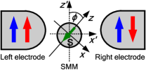
Figure 1: (color online) Schematic picture of the system under consideration for two collinear configurations of the leads’ magnetic moments: parallel (blue arrows) and antiparallel (red arrows). The axis $y$ ($y^{\prime}$) is normal to the $xz$ ($x^{\prime}z^{\prime}$) plane.

The full Hamiltonian of the system reads

$$\mathcal{H}=\mathcal{H}_{S\!M\!M}+\mathcal{H}_{L}+\mathcal{H}_{R}+\mathcal{H}_{T}.$$ (1)

The first term describes the free SMM and takes the form

$$\mathcal{H}_{S\!M\!M}=-DS_{z}^{2},$$ (2)

where $S_{z}$ is the $z$ component of the spin operator, and $D$ is the uniaxial anisotropy constant. The next two terms of the Hamiltonian $\mathcal{H}$ correspond to the two ferromagnetic electrodes,

$$\mathcal{H}_{q}=\sum_{{\bm{k}}\alpha}\epsilon_{{\bf k}\alpha}^{q}\>a_{{\bf k}\alpha}^{q{\dagger}}a_{{\bf k}\alpha}^{q}$$ (3)

for $q=L$ (left) and $q=R$ (right). The electrodes are represented by a band of non-interacting electrons with the energy dispersion $\epsilon_{{\bf k}\alpha}$, where $\bf k$ denotes a wave vector, $\alpha$ is the electron spin index ($\alpha=+$ for spin majority and $\alpha=-$ for spin minority electrons), and $a_{{\bf k}\alpha}^{q{\dagger}}$ ($a_{{\bf k}\alpha}^{q}$) is the relevant creation (anihilation) operator. Finally, the last term of the Hamiltonian $\mathcal{H}$ stands for the tunneling processes and is given by the Appelbaum Hamiltonian Appelbaum_PR17/66 rotated by the angle $\phi$ around the axis $y^{\prime}=y$ (see Fig. 1),

$$\mathcal{H}_{T} =\frac{1}{2}\sum_{qq^{\prime}}\sum_{{\bf k}{\bf k}^{\prime}\alpha\beta}\frac{J_{q,q^{\prime}}}{\sqrt{N_{q}\,N_{q^{\prime}}}}\>\bm{\sigma}_{\alpha\beta}\cdot\mathbf{S}\ \Bigg{\{}\cos^{2}{\frac{\phi}{2}}\ a_{{\bf k}\alpha}^{q{\dagger}}a_{{\bf k}^{\prime}\beta}^{q^{\prime}}\>+\>\sin^{2}{\frac{\phi}{2}}\ a_{{\bf k}\bar{\alpha}}^{q{\dagger}}a_{{\bf k}^{\prime}\bar{\beta}}^{q^{\prime}}\>-\>\frac{1}{2}\sin{\phi}\Big{(}a_{{\bf k}\alpha}^{q{\dagger}}a_{{\bf k}^{\prime}\bar{\beta}}^{q^{\prime}}+a_{{\bf k}\bar{\alpha}}^{q{\dagger}}a_{{\bf k}^{\prime}\beta}^{q^{\prime}}\Big{)}\Bigg{\}}$$

$$+\sum_{{\bf k}{\bf k}^{\prime}\alpha}\frac{T_{d}}{\sqrt{N_{L}\,N_{R}}}\>a_{{\bf k}\alpha}^{L{\dagger}}a_{{\bf k}^{\prime}\alpha}^{R}\>+\>H.c.,$$ (4)

where $\bm{\sigma}=(\sigma^{x},\sigma^{y},\sigma^{z})$ are the Pauli matrices, $\bm{S}$ is the SMM’s spin operator, and $\bar{\alpha}=-\alpha$. The first term in the above equation describes exchange interaction of the SMM and electrons in the leads, with $J_{q,q^{\prime}}$ denoting the relevant exchange parameter. For the sake of simplicity, we consider only symmetrical situation, where $J_{L,L}=J_{R,R}=J_{L,R}=J_{R,L}\equiv J$. The second term in Eq. (II) represents direct tunneling between the leads, with $T_{d}$ denoting the corresponding tunneling parameter. We also assume that $J$ and $T_{d}$ are independent of energy and polarization of the leads. Finally, $N_{q}$ ($q=L,R$) denote the number of elementary cells in the $q$-th electrode.

III Theoretical description

The electric current $I$ flowing through the system is determined with the use of the Fermi golden rule Kim_PRL92/04 ; Misiorny_PRB07 . Up to the leading terms with respect to the coupling constants $J$ and $T_{d}$, the current can be expressed by the formula

$$I =\frac{2\pi}{\hbar}\>e^{2}\>\Big{[}|T_{d}|^{2}+|J|^{2}\cos^{2}{\phi}\left\langle S_{z}^{2}\right\rangle\Big{]}\left(D_{\uparrow}^{L}D_{\uparrow}^{R}+D_{\downarrow}^{L}D_{\downarrow}^{R}\right)\>V$$

$$+\frac{2\pi}{\hbar}\>e\>|J|^{2}\>\sum_{m}P_{m}\sum_{\eta=+,-}A_{\eta}(m)\Bigg{\{}\eta\left[D_{\uparrow}^{L}D_{\downarrow}^{R}\cos^{4}{\frac{\phi}{2}}+D_{\downarrow}^{L}D_{\uparrow}^{R}\sin^{4}{\frac{\phi}{2}}\right]\zeta\big{(}D(\eta 2m+1)+\eta eV\big{)}$$

$$\hskip 139.41832pt-\eta\left[D_{\uparrow}^{L}D_{\downarrow}^{R}\sin^{4}{\frac{\phi}{2}}+D_{\downarrow}^{L}D_{\uparrow}^{R}\cos^{4}{\frac{\phi}{2}}\right]\zeta\big{(}D(\eta 2m+1)-\eta eV\big{)}$$

$$\hskip 128.0374pt+\frac{\sin^{2}{\phi}}{4}\left(D_{\uparrow}^{L}D_{\uparrow}^{R}+D_{\downarrow}^{L}D_{\downarrow}^{R}\right)\left[\zeta\big{(}D(\eta 2m+1)+\eta eV\big{)}+\zeta\big{(}D(\eta 2m+1)-\eta eV\big{)}\right]\Bigg{\}},$$ (5)

where $e$ is the electron charge (for simplicity assumed $e>0$, so the current is positive for electrons tunnelling from the left to right). In the above equation $D_{\sigma}^{q}$ is the density of states (DOS) at the Fermi level in the $q$-th electrode for spin $\sigma$, and $\left\langle S_{z}^{2}\right\rangle=\sum_{m}m^{2}P_{m}$, where $P_{m}$ denotes the probability of finding the SMM in the spin state $|m\rangle$. The voltage $V$ is defined as the difference of the leads’ electrochemical potentials, $eV=\mu_{L}-\mu_{R}$. Finally, we introduced the notation: $A_{\pm}(m)=S(S+1)-m(m\pm 1)$, and $\zeta(\epsilon)=\epsilon\big{[}1-\exp(-\epsilon\beta)\big{]}^{-1}$ with $\beta^{-1}=k_{B}T$.

To compute numerically the current $I$ from Eq. (III), one needs to know the probabilities $P_{m}$. To determine them, the SMM’s spin is assumed to be saturated in the initial state $|-S\rangle$, and then voltage growing linearly in time is applied Misiorny_PRB07 . Since the reversal process occurs through all the consecutive intermediate spin states, the probabilities can be found by solving the set of relevant master equations,

$$\left\{\begin{aligned} c\,\frac{dP_{m}}{dV}\>&=\>\sum_{l=-S}^{S}\Big{\{}\gamma_{\>l}^{-}\>\delta_{\>l,m+1}\>+\>\gamma_{\>l}^{+}\>\delta_{\>l,m-1}\>-\>\left(\gamma_{\>l}^{-}\>+\>\gamma_{\>l}^{+}\right)\>\delta_{\>l,m}\Big{\}}P_{\>l},\\ c\,\frac{dP_{\pm S}}{dV}\>&=\>-\>\gamma_{\pm S}^{\mp}\>P_{\pm S}\>+\>\gamma_{\pm S\mp 1}^{\pm}\>P_{\pm S\mp 1},\end{aligned}\right.$$ (6)

for $-S<m<S$, where $c=V/t$ is the speed at which the voltage is increased. The parameters $\gamma_{m}^{+(-)}$ describe the rates at which the spin $z$ component ($m$) is increased (decreased) by one. These tunneling rates have been calculated from the Fermi golden rule and have the form,

$$\gamma_{m}^{\pm} =\frac{2\pi}{\hbar}\>|J|^{2}\>A_{\pm}(m)\>\Bigg{\{}\cos^{4}{\frac{\phi}{2}}\Big{[}D_{\uparrow}^{L}D_{\downarrow}^{R}\>\zeta\big{(}D(\pm 2m+1)\pm eV\big{)}\>+\>D_{\downarrow}^{L}D_{\uparrow}^{R}\>\zeta\big{(}D(\pm 2m+1)\mp eV\big{)}\Big{]}$$

$$\hskip 77.67589pt+\>\sin^{4}{\frac{\phi}{2}}\Big{[}D_{\uparrow}^{L}D_{\downarrow}^{R}\>\zeta\big{(}D(\pm 2m+1)\mp eV\big{)}\>+\>D_{\downarrow}^{L}D_{\uparrow}^{R}\>\zeta\big{(}D(\pm 2m+1)\pm eV\big{)}\Big{]}$$

$$\hskip 77.67589pt+\>\frac{\sin^{2}\phi}{4}\Big{(}D_{\uparrow}^{L}D_{\uparrow}^{R}\>+\>D_{\downarrow}^{L}D_{\downarrow}^{R}\Big{)}\>\Big{[}\zeta\big{(}D(\pm 2m+1)+eV\big{)}\>+\>\zeta\big{(}D(\pm 2m+1)-eV\big{)}\Big{]}$$

$$+\>\left[\left(\sin^{4}{\frac{\phi}{2}}+\cos^{4}{\frac{\phi}{2}}\right)\left(D_{\uparrow}^{L}D_{\downarrow}^{L}+D_{\uparrow}^{R}D_{\downarrow}^{R}\right)\>+\>\frac{\sin^{2}\phi}{4}\left({D_{\uparrow}^{L}}^{2}+{D_{\downarrow}^{L}}^{2}+{D_{\uparrow}^{R}}^{2}+{D_{\downarrow}^{R}}^{2}\right)\right]\zeta\big{(}D(\pm 2m+1)\big{)}\Bigg{\}}.$$ (7)

IV Numerical results and discussion

Numerical results have been obtained for the molecule $\textrm{Fe}_{8}$ Gatteschi_AngewChem42/03 ; Wernsdorfer_Science284/99 corresponding to the total spin $S=10$, whose anisotropy constant is $D=0.292$ K. Apart from this, we assume $J\approx T_{d}\approx 100$ meV. Calculations have been performed for the temperature $T=0.01$ K, which is below the molecule’s blocking temperature $T_{B}=0.36$ K, and for $c=10$ kV/s. It has been also assumed that both the leads are made of the same metallic material characterized by the total DOS $D=D_{+}^{q}+D_{-}^{q}\approx 0.5$ per electron-volt and per elementary cell, where $D_{+(-)}^{q}$ denotes the DOS of majority (minority) electrons in the $q$-th electrode. Furthermore, the $q$-th electrode is described by the polarization parameter $P^{q}$ defined as $P^{q}=(D_{+}^{q}-D_{-}^{q})/(D_{+}^{q}+D_{-}^{q})$. The following discussion is limited to the case, where one electrode (the left one) is fully polarized, $P^{L}=1$, whereas the polarization factor of the second electrode can vary from $P^{R}=0$ (nonmagnetic) to $P^{R}=1$ (half-metallic ferromagnet).

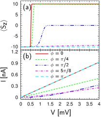
Figure 2: (color online) The average value of the SMM’s spin, $\langle S_{z}\rangle$, and the current $I$ flowing through the system as a function of the voltage $V$, calculated for the parallel configuration of the electrodes’ magnetic moments with $P^{L}=1$ and $P^{R}=0.3$.

In Fig. 2 we show the average value of the $z$-component of the SMM’s spin, $\langle S_{z}\rangle$, and the charge current $I$, calculated for several values of the angle $\phi$ and for parallel magnetic configuration of the leads. The case of $\phi=0$ ($\phi=\pi$) corresponds to the situation when the initial SMM’s spin is antiparallel (parallel) to the leads’ spin moments. One can note that the influence of current on the molecule’s spin gradually disappears as the angle $\phi$ approaches $\pi$. For $\phi<\pi/2$, the molecule’s spin becomes switched from the state $|-S\rangle$ to the state $|S\rangle$. The switching time, however, becomes longer and longer as the angle $\phi$ approaches $\phi=\pi/2$. At $\phi=\pi/2$, which corresponds to the situation with the SMM’s easy axis perpendicular to the leads’ magnetic moments, different molecular spin states $|m\rangle$ become equally probable with increasing voltage, and therefore $\langle S_{z}\rangle\rightarrow 0$. This is a consequence of the fact that when the voltage exceeds the activation energy for the spin-flip process Misiorny_PRB07 , the SMM undergoes transitions to upper and lower spin states with equal rates $\gamma_{m}^{+}=\gamma_{m}^{-}$ (see Eq. (III)).

When $\phi>\pi/2$, the spin state of the molecule is only weakly modified by current, and remains strictly unchanged for $\phi=\pi$. The absence of switching by positive current at large values of $\phi$ (for the assumed parameters) is consistent with the conclusion of Ref. [6], where for collinear configurations and positive current only switching from $|-S\rangle$ to $|S\rangle$ states was allowed, whereas positive current had no influence on the state $|S\rangle$.

The SMM’s spin can be reversed due to exchange interaction with tunneling electrons. The latter flip their spins and hence add to or subtract some amount of angular momentum from the molecule. As the angle $\phi$ grows, the spin orientation of tunneling electrons ‘seen’ by the molecule and consequently also the transition rates given by Eq. (III) change as well. Figure 2b shows the current flowing in the system as a function of the bias voltage. This current strongly depends on the orientation of the SMM’s easy axis. This dependence is a consequence of the fact that the dominant contribution to current is due to the exchange term (first term in Eq. (II)), which is sensitive to the orientation of the SMM’s spin. The curves for $\phi=0$ and $\phi=\pi$ overlap (except for a small voltage range where the switching for $\phi=0$ takes place – not resolved in Fig. 2b).

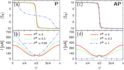
Figure 3: (color online) The average value of the SMM’s spin $\langle S_{z}\rangle$ (a), and the current $I$ flowing through the system (b) as a function of the angle $\phi$ in the parallel (P) (a,b) and antiparallel (AP) (c,d) magnetic configurations for $V=2$ mV and $P^{L}=1$.

Figure 3 presents the spin $z$-component $\langle S_{z}\rangle$ and the current $I$ in both configurations of the leads’ magnetic moments, plotted as a function of the angle $\phi$ and calculated for $V=2$ mV. For $\phi<\pi/2$, the spin switching takes place in both parallel and antiparallel magnetic configurations. Figure 3 also indicates that the current at $\phi=\pi/2$ is independent of the magnetic configuration as well as on the polarization parameters of the leads.

In conclusion, we have shown that tilting the easy axis of a SMM from the collinear orientation relative to the leads’ magnetic moments has a significant influence on the reversal process of the molecule’s spin, as well as on current flowing through the system.

Acknowledgements This work was supported by funds from the Ministry of Science and Higher Education as a research project in years 2006-2009. One of us (MM) also acknowledges support from the MAGELMAT network.

References

- (1) D. Gatteschi and R. Sessoli, Angew. Chem. Int. Ed. 42, 268 (2003).
- (2) C. Joachim, J. K. Gimzewski and A. Aviram, Nature 408, 541 (2000).
- (3) C. Timm and F. Elste, Phys. Rev. B 73, 235304 (2006).
- (4) G.-H. Kim and T.-S. Kim, Phys. Rev. Lett. 92, 137203 (2004).
- (5) F. Elste and C. Timm , Phys. Rev. B 73, 235305 (2006).
- (6) M. Misiorny and J. Barnaś , Phys. Rev. B 75, 134425 (2007).
- (7) F. Elste and C. Timm, cond-mat/0611108.
- (8) H. B. Heersche et al., Phys. Rev. Lett. 96, 206801 (2006).
- (9) M.-H. Jo et al., Nano Lett. 6, 2014 (2006).
- (10) J. J. Henderson et al., cond-mat/0703013.
- (11) C. Timm, cond-mat/0702220.
- (12) J. Appelbaum, Phys. Rev. 17, 91 (1966).
- (13) W. Wernsdorfer and R. Sessoli, Science 284, 133 (1999).