Effective interactions and large-scale diagonalization for quantum dots

Abstract

The widely used large-scale diagonalization method using harmonic oscillator basis functions (an instance of the Rayleigh-Ritz method, also called a spectral method, configuration-interaction method, or “exact diagonalization” method) is systematically analyzed using results for the convergence of Hermite function series. We apply this theory to a Hamiltonian for a one-dimensional model of a quantum dot. The method is shown to converge slowly, and the non-smooth character of the interaction potential is identified as the main problem with the chosen basis, while on the other hand its important advantages are pointed out. An effective interaction obtained by a similarity transformation is proposed for improving the convergence of the diagonalization scheme, and numerical experiments are performed to demonstrate the improvement. Generalizations to more particles and dimensions are discussed.

I Introduction

Large-scale diagonalization is widely used in many areas of physics, from quantum chemistryHelgaker et al. (2000) to nuclear physics.Caurier et al. (2005) It is also routinely used to obtain spectra of model quantum dots, see for example Refs. Ezaki et al., 1997; Maksym, 1998; Bruce and Maksym, 2000; Creffield et al., 1999; Häusler and Kramer, 1993; Reimann et al., 2000; Rontani et al., 2006; Ciftja and Faruk, 2006; Jauregui et al., 1993; Imamura et al., 1999; Tavernier et al., 2003; Wensauer et al., 2004; Helle et al., 2005; Xie, 2006; Tavernier et al., 2006; Gylfadottir et al., 2006. The method is based on a projection of the model Hamiltonian onto a finite-dimensional subspace of the many-body Hilbert space in question, hence the method is an instance of the Rayleigh-Ritz method.Gould (1995) Usually, one takes the stance that the many-body Hamiltonian is composed of two parts $\hat{H}_{0}$ and $\hat{H}_{1}$, treating the latter as a perturbation of the former, whose eigenfunctions are assumed to be a basis for the Hilbert space. This leads to a matrix diagonalization problem, hence the name of the method. As $\hat{H}_{1}$ often contains the interaction terms of the model, “perturbing” the electronic configuration states of $\hat{H}_{0}$, the method is also called the configuration-interaction method. In the limit of an infinite basis, the method is in principle exact, and for this reason it is also called “exact diagonalization”. Usually, however, this method is far from exact, as $\hat{H}_{1}$ is rarely a small perturbation (in a sense to be specified in Sec. III.5) while limited computing resources yield a tight bound on the number of degrees of freedom available per particle.

In this work we provide mathematical convergence criteria for configuration-interaction calculations. More specifically, we address this problem in the case where $\hat{H}_{0}$ is a harmonic oscillator (or h.o. for short), concentrating on a simple one-dimensional problem. A common model for a quantum dot is indeed a perturbed harmonic oscillator, and using h.o. basis functions is also a common approach in other fields of many-body physics and partial differential equations settings in general, as it is also known as the Hermite spectral method.Tang (1993) When we in the following refer to the configuration-interaction method, or CI for short, it is assumed that a h.o. basis is used.

Studying a one-dimensional problem may seem unduly restrictive, but will in fact enable us to treat realistic multidimensional problems as well due to the symmetries of the harmonic oscillator. Moreover, we choose a worst-case scenario, in which the interaction potential decays very slowly. We argue that the nature of the perturbation $\hat{H}_{1}$, i.e., the non-smooth character of the Coulomb potential or the trap potential, hampers the convergence properties of the method. To circumvent this problem and improve the convergence rate, we construct an effective two-body interaction via a similarity transformation. This approach, also using a h.o. basis, is routinely used in nuclear physics,Navrátil and Barrett (1998); Navrátil et al. (2000, 2000) where the interactions are of a completely different nature.

The effective interaction is defined for a smaller space than the original Hilbert space, but it reproduces exactly the lowest-lying eigenvalues of the full Hamiltonian. This can be accomplished by a technique introduced by Suzuki, Okamoto and collaborators.Suzuki (1982); suz ; Suzuki and Okamoto (1995, 1994) Approaches based on this philosophy for deriving effective interactions have been used with great success in the nuclear many-body problem.Navrátil and Barrett (1998); Navrátil et al. (2000, 2000) For light nuclei it provides benchmark calculations of the same quality as Green’s function Monte Carlo methods or other ab initio methods. See for example Ref. Kamada et al., 2001 for an extensive comparison of different methods for computing properties of the nucleus ⁴He. It was also used in a limited comparative study of large-scale diagonalization techniques and stochastic variational methods applied to quantum dots.Varga et al. (2001)

We demonstrate that this approach to the CI method for quantum dots yields a considerable improvement to the convergence rate. This has important consequences for studies of the time-development of quantum dots with two or more electrons, as reliable calculations of the eigenstates are crucial ingredients in studies of coherence. This is of particular importance in connection with the construction of quantum gates based on quantum dots.Loss and DiVincenzo (1998) Furthermore, the introduction of an effective interaction allows for studies of many-electron quantum dots via other many-body methods like resummation schemes such as various coupled cluster theories as well. As the effective interaction is defined only within the model space, systematic and controlled convergence studies of these methods in terms of the size of this space is possible.

The article is organized as follows: In Sec. II the model quantum dot Hamiltonian is discussed. In Sec. III we discuss the CI method and its numerical properties. Central to this section are results concerning the convergence of Hermite function series.Boyd (1984); Hille (1939) We also demonstrate the results with some numerical experiments.

In Sec. IV we discuss the similarity transformation technique of Suzuki and collaboratorsSuzuki (1982); suz ; Suzuki and Okamoto (1995, 1994) and replace the Coulomb term in our CI calculations with this effective interaction. We then perform numerical experiments with the new method and discuss the results.

We conclude the article with generalizations to more particles in higher dimensions and possible important applications of the new method in Sec. V.

II One-dimensional quantum dots

A widely used model for a quantum dot containing $N$ charged fermions is a perturbed harmonic oscillator with Hamiltonian

$$\hat{H} = \sum_{j=1}^{N}\Big{(}-\frac{1}{2}\nabla_{j}^{2}+\frac{1}{2}\|\vec{r}_{j}\|^{2}+v(\vec{r}_{j})\Big{)}$$ (1)

$$+\sum_{j=1}^{N}\sum_{k=j+1}^{N}U(\|r_{j}-r_{k}\|),$$

where $\vec{r}_{j}\in\mathbb{R}^{2}$, $j=1,\ldots,N$ are each particle’s spatial coordinate, $v(\vec{r})$ is a small modification of the h.o. potential $\|\vec{r}\|^{2}/2$, and $U(r)$ is the Coulomb interaction, viz, $U(r)=\lambda/r$. Modelling the quantum dot geometry by a perturbed harmonic oscillator is justified by self-consistent calculations,Kumar et al. (1990); Macucci et al. (1997); Maksym and Bruce (1997) and is the stance taken by many other authors using the large-scale diagonalization technique as well.Ezaki et al. (1997); Maksym (1998); Imamura et al. (1999); Bruce and Maksym (2000); Reimann et al. (2000); Tavernier et al. (2003); Wensauer et al. (2004); Helle et al. (2005); Ciftja and Faruk (2006); Rontani et al. (2006); Xie (2006); Tavernier et al. (2006)

Electronic structure calculations amount to finding eigenpairs $(E,\Psi)$, e.g., the ground state energy and wave function, such that

$$\hat{H}\Psi=E\Psi,\quad\Psi\in\mathcal{H}\text{ and }E\in\mathbb{R}.$$

Here, even though the Hamiltonian only contains spatial coordinates, the eigenfunction $\Psi$ is a function of both the spatial coordinates $\vec{r}_{k}\in\mathbb{R}^{2}$ and the spin degrees of freedom $\sigma_{k}\in\{-1/2,+1/2\}$, i.e.,

$$\mathcal{H}=L_{2}(\mathbb{R}^{2N})\otimes\mathbb{C}^{2}.$$

The actual Hilbert space is the space of the antisymmetric functions, i.e., functions $\Psi$ for which

$$\Psi(x_{P(1)},x_{P(2)},\ldots,x_{P(N)})=\operatorname{sgn}(P)\Psi(x_{1},x_{2},\ldots,x_{N}),$$

for all permutations $P$ of $N$ symbols. Here, $x_{k}=(\vec{r}_{k},\sigma_{k})$.

For simplicity, we concentrate on one-dimensional quantum dots. Even though this is not an accurate model for real quantum dots, it offers several conceptual and numerical advantages. Firstly, the symmetries of the harmonic oscillator makes the numerical properties of the configuration-interaction method of this system very similar to a two or even three-dimensional model, as the analysis extends almost directly through tensor products. Secondly, we may investigate many-body effects for moderate particle numbers $N$ while still allowing a sufficient number of h.o. basis functions for unambiguously addressing accuracy and convergence issues in numerical experiments.

In this article, we further focus on two-particle quantum dots. Incidentally, for the two-particle case one can show that the Hilbert space of anti-symmetric functions is spanned by functions on the form

$$\Psi(\vec{r}_{1},\sigma_{1},\vec{r}_{2},\sigma_{2})=\psi(\vec{r}_{1},\vec{r}_{2})\chi(\sigma_{1},\sigma_{2}),$$

where the spin wave function $\chi$ can be taken as symmetric or antisymmetric with respect to particle exchange, leading to an antisymmetric or symmetric spatial wave function $\psi$, respectively. Inclusion of a magnetic field $\vec{B}$ poses no additional complications,Wensauer et al. (2003) but for simplicity we presently omit it. Thus, it is sufficient to consider the spatial problem and produce properly symmetrized wavefunctions.

Due to the peculiarities of the bare Coulomb potential in one dimensionKurasov (1996); Gesztesy (1980) we choose a screened approximation $U(x_{1}-x_{2};\lambda,\delta)$ given by

$$U(x;\lambda,\delta)=\frac{\lambda}{|x|+\delta},$$

where $\lambda$ is the strength of the interaction and $\delta>0$ is a screening parameter which can be interpreted as the width of the wave function orthogonal to the axis of motion. This choice is made since it is non-smooth, like the bare Coulomb potential in two and three dimensions. The total Hamiltonian then reads

$$\hat{H} = -\frac{1}{2}\Big{(}\frac{\partial^{2}}{\partial x_{1}^{2}}+\frac{\partial^{2}}{\partial x_{2}^{2}}\Big{)}+\frac{1}{2}(x_{1}^{2}+x_{2}^{2})+$$ (2)

$$v(x_{1})+v(x_{2})+U(x_{1}-x_{2};\lambda,\delta).$$

Observe that for $U=0$, i.e., $\lambda=0$, the Hamiltonian is separable. The eigenfunctions of $\hat{H}$ (disregarding proper symmetrization due to the Pauli principle) become $\psi_{n_{1}}(x_{1})\psi_{n_{2}}(x_{2})$, where $\psi_{n}(x)$ are the eigenfunctions of the trap Hamiltonian $\hat{H}_{\text{t}}$ given by

$$\hat{H}_{\text{t}}=-\frac{1}{2}\frac{\partial^{2}}{\partial x^{2}}+\frac{1}{2}x^{2}+v(x).$$ (3)

Similarly, for a vanishing trap modification $v(x)=0$ the Hamiltonian is separable in (normalized) centre-of-mass coordinates given by

$$X=\frac{x_{1}+x_{2}}{\sqrt{2}}\quad\text{and}\quad x=\frac{x_{1}-x_{2}}{\sqrt{2}}.$$

Indeed, any orthogonal coordinate change leaves the h.o. Hamiltonian invariant (see Sec. III), and hence

$$\hat{H} = -\frac{1}{2}\Big{(}\frac{\partial^{2}}{\partial X^{2}}+\frac{\partial^{2}}{\partial x^{2}}\Big{)}+\frac{1}{2}(X^{2}+x^{2})+$$

$$v\big{(}(X+x)/\sqrt{2}\big{)}+v\big{(}(X-x)/\sqrt{2}\big{)}+U(\sqrt{2}x;\lambda,\delta).$$

The eigenfunctions become $\phi_{n}(X)\psi_{m}(x)$, where $\phi_{n}(X)$ are the Hermite functions, i.e., the eigenfunctions of the h.o. Hamiltonian (see Sec. III), and where $\psi_{m}(x)$ are the eigenfunctions of the interaction Hamiltonian, viz,

$$\hat{H}_{\text{i}}=-\frac{1}{2}\frac{\partial^{2}}{\partial x^{2}}+\frac{1}{2}x^{2}+U(\sqrt{2}x;\lambda,\delta).$$ (4)

Odd (even) functions $\psi_{m}(x)$ yield antisymmetric (symmetric) wave functions with respect to particle interchange.

III Configuration-interaction method

III.1 The harmonic oscillator and model spaces

The configuration-interaction method is an instance of the Rayleigh-Ritz method,Gould (1995) employing eigenfunctions of the unperturbed h.o. Hamiltonian as basis for a finite dimensional Hilbert space $\mathcal{P}$, called the model space, onto which the Hamiltonian (1), or in our simplified case, the Hamiltonian (2), is projected and then diagonalized. As mentioned in the Introduction, this method is in principle exact, if the basis is large enough.

We write the $N$-body Hamiltonian (1) as

$$\hat{H}=\hat{H}_{0}+\hat{H}_{1},$$

with $\hat{H}_{0}$ being the h.o. Hamiltonian, viz,

$$\hat{H}_{0}=-\frac{1}{2}\sum_{j=1}^{N}\nabla^{2}_{j}+\frac{1}{2}\sum_{j=1}^{N}\|\vec{r}_{j}\|^{2},$$

and $\hat{H}_{1}$ being a perturbation of $\hat{H}_{0}$, viz,

$$\hat{H}_{1}=\sum_{j=1}^{N}v(\vec{r}_{j})+\sum_{j=1}^{N}\sum_{k=j+1}^{N}U(\|r_{j}-r_{k}\|).$$

For a simple one-dimensional model of two particles we obtain

$$\hat{H}_{0}=\hat{h}(x_{1})+\hat{h}(x_{2}),$$

where $\hat{h}(x)$ is the well-known one-dimensional harmonic oscillator Hamiltonian, viz,

$$\hat{h}(x)=-\frac{1}{2}\frac{\partial^{2}}{\partial x^{2}}+\frac{1}{2}x^{2}.$$

Clearly, $\hat{H}_{0}$ is just a two-dimensional h.o. Hamiltonian, if we disregard symmetrization due to the Pauli principle. For the perturbation, we have

$$\hat{H}_{1}=v(x_{1})+v(x_{2})+\frac{\lambda}{|x_{1}-x_{2}|+\delta}.$$

In order to do a more general treatment, let us recall some basic facts about the harmonic oscillator.

If we consider a single particle in $D$-dimensional space, it is clear that the $D$-dimensional harmonic oscillator Hamiltonian is the sum of one-dimensional h.o. Hamiltonians for each Euclidean coordinate, viz,

$$\hat{h}^{(D)}=-\frac{1}{2}\nabla^{2}+\frac{1}{2}\|\vec{x}\|^{2}=\sum_{k=1}^{D}\hat{h}(x_{k}).$$ (5)

We indicate the variables on which the operators depend by parenthesis if there is danger of confusion. Moreover, the h.o. Hamiltonian for $N$ (distinguishable) particles in $d$ dimensions is simply $\hat{h}^{(Nd)}$. The $D$-dimensional h.o. Hamiltonian is manifestly separable, and the eigenfunctions are

$$\Phi_{\vec{n}}(\vec{x})=\prod_{k=1}^{D}\phi_{n_{k}}(x_{k})$$

with energies

$$\epsilon_{\vec{n}}=\frac{D}{2}+\sum_{k=1}^{D}n_{k},$$

where $\vec{n}$ denotes the multi-index of quantum numbers $n_{k}$. The one-dimensional h.o. eigenfunctions are given by

$$\phi_{n}(x)=\big{(}2^{n}n!\pi^{1/2}\big{)}^{-1/2}H_{n}(x)e^{-x^{2}/2},$$

where $H_{n}(x)$ are the usual Hermite polynomials. These functions are the Hermite functions and are treated in further detail in Sec. III.3.

As for the discretization of the Hilbert space, we employ a so-called energy-cut model space $\mathcal{P}$, defined by the span of all h.o. eigenfunctions with energies up to a given $\epsilon=N_{\text{max}}+D/2$, viz,

$$\mathcal{P}:=\operatorname{sp}\big{\{}\Phi_{\vec{n}}(\vec{x})\;\big{|}\;0\leq\sum_{k}n_{k}\leq N_{\text{max}}\big{\}},$$

where we bear in mind that the $D=Nd$ dimensions are distributed among the $N$ particles.

For the one-dimensional model with only one particle, the model space reduces to

$$\mathcal{P}_{1}=\operatorname{sp}\big{\{}\phi_{n}(x)\;\big{|}\;0\leq n\leq N_{\text{max}}\big{\}}.$$ (6)

Thus, one particle is associated with one integer quantum number $n$, denoting the “shell number where the particle resides”, in typical terms. For two particles, we get

$$\mathcal{P}_{2}=\operatorname{sp}\big{\{}\phi_{n_{1}}(x_{1})\phi_{n_{2}}(x_{2})\;\big{|}\;0\leq n_{1}+n_{2}\leq N_{\text{max}}\big{\}}.$$

We illustrate this space in Fig. 1.

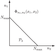
Figure 1: Two-body model space defined by a cut in energy. The two-body state has quantum numbers $n_{1}$ and $n_{2}$, the sum of which does not exceed $N_{\text{max}}$.

Proper symmetrization must also be applied. However, the Hamiltonian (1) commutes with particle permutations, meaning that the eigenfunctions will be symmetric or antisymmetric, assuming that the eigenvalues are distinct. In the case of degeneracy, we may simply produce (anti)symmetric eigenfunctions by taking linear combinations.

We mention that other model spaces can also be used; most common is perhaps the direct product model space, defined by $N$ direct products of $\mathcal{P}_{1}$ rather than a cut in energy as above.

III.2 Coordinate changes and the h.o.

It is obvious that any orthogonal coordinate change $\vec{y}=S\vec{x}$ where $S^{T}S=1$ commutes with $\hat{h}^{(D)}$. In particular, energy is conserved under the coordinate change. Therefore, the eigenfunctions of the transformed Hamiltonian will be a linear combination of the original eigenfunctions of the same energy, viz,

$$\Phi_{\vec{n}}(S\vec{x})=\sum_{\vec{n}^{\prime}}\langle\Phi_{\vec{n}^{\prime}},\hat{T}\Phi_{\vec{n}}\rangle\Phi_{\vec{n}^{\prime}}(\vec{x}),$$

where the sum is over all $\vec{n}^{\prime}$ such that $\epsilon_{\vec{n}^{\prime}}=\epsilon_{\vec{n}}$. Here, $\hat{T}$ performs the coordinate change, viz,

$$\hat{T}\Phi_{\vec{n}}(\vec{x})=\Phi_{\vec{n}}(S\vec{x}),$$ (7)

where $\hat{T}$ is unitary. Also note that energy conservation implies that $\mathcal{P}$ is invariant with respect to the coordinate change, implying that the CI method is equivalent in the two coordinate systems.

An important example is the centre-of-mass transformation introduced in Sec. II. This transformation is essential when we want to compute the Hamiltonian matrix since the interaction is given in terms of these coordinates.

Observe that in the case when the Hamiltonian is in fact separated by such a coordinate change, the formulation of the exact problem using h.o. basis is equivalent to two one-particle problems using h.o. basis in the new coordinates.

III.3 Approximation properties of the Hermite functions

In order to understand the accuracy of the CI method, we need to study the approximation properties of the Hermite functions. Note that all the Hermite functions $\phi_{n}(x)$ spanning $L_{2}(\mathbb{R})$ are smooth. Indeed, they are holomorphic in the entire complex plane. Any finite linear combination of these will yield another holomorphic function, so any non-smooth function will be badly approximated. This simple fact is sadly neglected in the configuration-interaction literature, and we choose to stress it here: Even though the Hermite functions are simple to compute and deal with, arising in a natural way from the consideration of a perturbation of the h.o. and obeying a wealth of beautiful relations, they are not very well suited for computation of functions whose smoothness is less than infinitely differentiable, or whose decay behaviour for large $|x|$ is algebraic, i.e., $f(x)=o(|x|^{\beta})$ for some $\beta<0$. Due to the direct product nature of the $N$-body basis functions, it is clear that these considerations are general, and not restricted to the one-dimensional one-particle situation.

Consider an expansion $\psi(x)=\sum_{n=0}^{\infty}c_{n}\phi_{n}(x)$ in Hermite functions of an arbitrary $\psi\in L_{2}(\mathbb{R})$. The coefficients are given by

$$c_{n}=\langle\phi_{n},\psi\rangle=\int_{-\infty}^{\infty}\psi(x)\bar{H}_{n}(x)e^{-x^{2}/2}\;\mathrm{d}x.$$

Here, $\bar{H}_{n}(x)=(2^{n}n!\sqrt{\pi})^{-1/2}H_{n}(x)$ are the normalized Hermite polynomials. If $\psi(x)$ is well approximated by the basis, the coefficients $c_{n}$ will decay quickly with increasing $n$. The least rate of convergence is a direct consequence of

$$\|\psi\|^{2}=\sum_{n=0}^{\infty}|c_{n}|^{2}<\infty,$$

hence we must have $|c_{n}|=o(n^{-1/2})$. (This is not a sufficient condition, however.) With further restrictions on the behaviour of $\psi(x)$, the decay will be faster. This is analogous to the faster decay of Fourier coefficients for smoother functions,Tveito and Winther (2002) although for Hermite functions, smoothness is not the only parameter as we consider an infinite domain. In this case, another equally important feature is the decay of $\psi(x)$ as $|x|$ grows, which is intuitively clear given that all the Hermite functions decay as $\exp(-x^{2}/2)$.

Let us prove this assertion. We give here a simple argument due to Boyd (Ref. Boyd, 1984), but we strengthen the result somewhat.

To this end, assume that $\psi(x)$ has $k$ square integrable derivatives (in the weak sense) and that $x^{m}\psi(x)$ is square integrable for $m=0,1,\ldots,k$. Note that this is a sufficient condition for

$$a^{\dagger}\psi(x)=\frac{1}{\sqrt{2}}(x\psi(x)-\psi^{\prime}(x)),$$

and $(a^{\dagger})^{2}\psi(x)$ up to $(a^{\dagger})^{k}\psi(x)$ to be square integrable as well. Here, $a^{\dagger}$ and its Hermitian conjugate $a$ are the well-known ladder operators for the harmonic oscillator.Mota et al. (2002)

Using integration by parts, the formula for $c_{n}$ becomes

$$c_{n} =\int_{-\infty}^{\infty}\psi(x)\bar{H}_{n}(x)e^{-x^{2}/2}\;\mathrm{d}x$$

$$=-(n+1)^{-1/2}\int_{-\infty}^{\infty}[a^{\dagger}\psi(x)]\bar{H}_{n+1}(x)e^{-x^{2}/2}\;\mathrm{d}x,$$

or

$$c_{n}=-(n+1)^{-1/2}d_{n+1},$$

where $d_{n}$ are the Hermite expansion coefficients of $a^{\dagger}\psi(x)\in L_{2}$. Since $\sum|d_{n}|^{2}<\infty$ by assumption, we obtain

$$\sum_{n=0}^{\infty}n|c_{n}|^{2}<\infty,$$

implying

$$c_{n}=o(n^{-1}).$$

Repeating this argument $k$ times, we obtain the estimate

$$c_{n}=o(n^{-(k+1)/2}).$$

It is clear that if $\psi(x)$ is infinitely differentiable, and if in addition $\psi(x)$ decays faster than any power of $x$, such as for example exponentially decaying functions, or functions behaving like $\exp(-\alpha x^{2})$, $c_{n}$ will decay faster than any power of $1/n$, so-called “infinite-order convercence,” or “spectral convergence.” Indeed, Hille (Ref. Hille, 1939) gives results for the decay of the Hermite coefficients for a wide class of functions. The most important for our application being the following: If $\psi(x)$ decays as $\exp(-\alpha x^{2})$, with $\alpha>0$, and if $\tau>0$ is the distance from the real axis to the nearest pole of $\psi(x)$ (when considered as a complex function), then

$$|c_{n}|=O(n^{-1/4}e^{-\tau\sqrt{2n+1}}),$$ (8)

a very rapid decay for even moderate $\tau$.

An extremely useful propertyBoyd (1984) of the Hermite functions is the fact that they are uniformly bounded, viz,

$$|\phi_{n}(x)|\leq 0.816,\quad\forall x,n.$$

As a consequence, the pointwise error in a truncated series is almost everywhere bounded by

$$|\psi(x)-\sum_{n=0}^{N_{\text{max}}}c_{n}\phi_{n}(x)|\leq 0.816\sum_{n=N_{\text{max}}+1}^{\infty}|c_{n}|.$$

Thus, estimating the error in the expansion amounts to estimating the sum of the neglected coefficients. If $|c_{n}|=o(n^{\alpha})$,

$$|\psi(x)-\sum_{n=0}^{N_{\text{max}}}c_{n}\phi_{n}(x)|=o(N_{\text{max}}^{\alpha+1}),\quad\text{a.e.}$$

For the error in the mean,

$$\|\psi(x)-\sum_{n=0}^{N}c_{n}\phi_{n}(x)\|=O(N_{\text{max}}^{\alpha+1/2}),$$ (9)

as is seen by approximating $\sum_{n=N_{\text{max}}+1}^{\infty}|c_{n}|^{2}$ by an integral.

In the above, “almost everywhere”, or “a.e.” for short, refers to the fact that we do not distinguish between square integrable functions that differ on a point set of Lebesgue measure zero. Moreover, there is a subtle distinction between the notations $O(g(n))$ and $o(g(n))$. For a given function $f$, $f(n)=o(g(n))$ if $\lim_{n\rightarrow\infty}|f(n)/g(n)|=0$, while $f(n)=O(g(n))$ if we have $\lim_{n\rightarrow\infty}|f(n)/g(n)|<\infty$; a slightly weaker statement.

III.4 Application to the interaction potential

Let us apply the above results to the eigenproblem for a perturbed one-dimensional harmonic oscillator, i.e.,

$$\psi^{\prime\prime}(x)=[x^{2}+2f(x)-2E]\psi(x),$$ (10)

which is also applicable when the two-particle Hamiltonian (2) is separable, i.e., when $U=0$ or $v=0$.

It is now clear that under the assumption that $f(x)$ is $k$ times differentiable (in the weak sense), and that $f(x)=o(|x|^{2})$ as $|x|\rightarrow\infty$, the eigenfunctions will be $k+2$ times (weakly) differentiable and decay as $\exp(-x^{2}/2)$ for large $|x|$. Hence, the Hermite expansion coefficients of $\psi(x)$ will decay as $o(n^{\alpha})$, $\alpha=-(k+3)/2$.

If we further assume that $f(x)$ is analytic in a strip of width $\tau>0$ around the real axis, the same will be true for $\psi(x)$, such that we can use Eq. (8) to estimate the coefficients.

A word of caution is however at its place. Although we have argued that if a given function can be differentiated $k$ times (in the weak sense) then the coefficients decay as $o(n^{\alpha})$, $\alpha=-(k+1)/2$, it may happen that this decay “kicks in” too late to be observable in practical circumstances.

Consider for example the following function:

$$g(x)=\frac{e^{-x^{2}/2}}{|x|+\delta},$$

which has exactly one (almost everywhere continuous) derivative and decays as $\exp(-x^{2}/2)$. However, the derivative is seen to have a jump discontinuity of magnitude $2/\delta^{2}$ at $x=0$. From the theory, we expect $o(n^{-1})$ decay of the coefficients, but for small $\delta$ the first derivative is badly approximated, so we expect to observe only $o(n^{-1/2})$ decay for moderate $n$, due to the fact that the rate of decay of the coefficients of $g(x)$ are explicitely given in terms of the coefficients of $a^{\dagger}g(x)$.

In Fig. 2 the decay rates at different $n$ and for various $\delta$ are displayed. The decay rate $\alpha$ is computed by estimating the slope of the graph of $\ln|c_{n}|$ versus $\ln n$, a technique used thoughout this article. Indeed, for small $\delta$ we observe only $\alpha\approx-1/2$ convergence in practical settings, where $n$ is moderate, while larger $\delta$ gives $\alpha\approx-1$ even for small $n$.

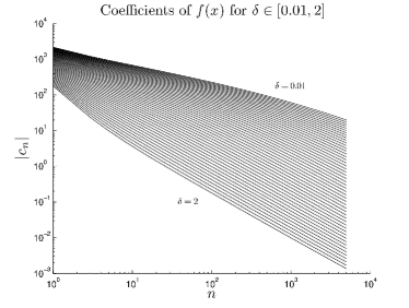
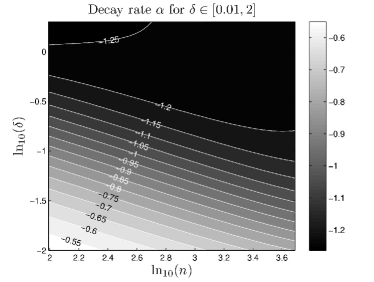
Figure 2: (Left) Coefficients $|c_{n}|$ of the function $\exp(-x^{2}/2)/(|x|+\delta)$ for $\delta\in[0.01,2]$, $n=0,2,\ldots,5000$. (Right) Estimated decay rate $\alpha$ of $|c_{n}|$, i.e., slope of the graphs in the left panel.

The above function was chosen due to its relation to the interaction Hamiltonian (4). Indeed, its coefficients are given by

$$c_{n}=\langle\phi_{n},g\rangle=\langle\phi_{n},U(x;1,\delta)\phi_{0}\rangle,$$

i.e., the proportional to the first row of the interaction matrix. Moreover, due to Eq. (10), the ground state $\psi$ of the interaction Hamiltonian has a second derivative with similar behaviour near $x=0$ as $g(x)$. Thus, we expect to observe $\alpha\approx-3/2$, rather than $\alpha\approx-2$, for the available range of $n$ in the large-scale diagonalization experiments.

We remark here, that it is quite common to model quantum dot systems using non-smooth potentialsWensauer et al. (2000) $v(\vec{r})$, and even to use the CI method with h.o. basis functions on these models.Harju et al. (2002); Helle et al. (2005); Førre et al. (2006)

III.5 Numerical experiments

We wish to apply the above analysis by considering the model Hamiltonian (2). We first consider the case where $v(x)=0$ or $U(x)=0$, respectively, which reduces the two-particle problem to one-dimensional problems through separation of variables, i.e., the diagonalization of the trap Hamiltonian $\hat{H}_{\text{t}}$ and the interaction Hamiltonian $\hat{H}_{\text{i}}$ in Eqs. (3) and (4). Then we turn to the complete non-separable problem.

For simplicity we consider the trap $x^{2}/2+v(x)$ with

$$v(x)=Ae^{-C(x-\mu)^{2}},\quad A,C>0,\mu\in\mathbb{R},$$

which gives rise to a double-well potential or a single-well potential, depending on the parameters, as depicted in Fig. 3. The perturbation is everywhere analytic and rapidly decaying. This indicates that the corresponding configuration-interaction energies and wave functions also should converge rapidly. In the below numerical experiments, we use $A=4$, $C=2$ and $\mu=0.75$, creating the asymmetric double well in Fig. 3.

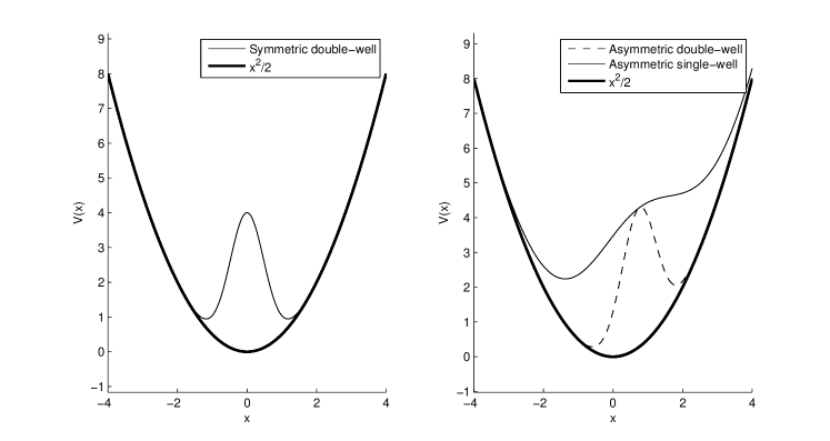
Figure 3: Left: Symmetric double-well potential created with the Gaussian perturbation $A\exp[-C(x-\mu)^{2}]$ with $A=4$, $\mu=0$ and $C=2$. Right: Asymmetric double-well potential created with the Gaussian perturbation with $A=4$, $\mu=0.75$ and $C=2$, and single-well potential using $C=0.25$.

For the interaction Hamiltonian $\hat{H}_{\text{i}}$ and its potential $x^{2}/2+U(\sqrt{2}x;\lambda,\delta)$ we arbitrarily choose $\lambda=1$ and $\delta=0.01$, giving a moderate jump discontinuity in the derivative.

As these problems are both one-dimensional, the model space reduces to $\mathcal{P}_{1}$ as given in Eq. (6). Each problem then amounts to diagonalizing a matrix $\mathbf{H}$ with elements

$$\mathbf{H}_{n,m}=\langle\phi_{n},\hat{H}_{\text{t,i}}\phi_{m}\rangle=\big{(}n+\frac{1}{2}\big{)}\delta_{n,m}+\int_{-\infty}^{\infty}\phi_{n}(x)f(x)\phi_{m}(x)\;\mathrm{d}x,\quad 0\leq n,m\leq N_{\text{max}},$$

with $f(x)=v(x)$ or $f(x)=U(\sqrt{2}x;1,0.01)$. We compute the matrix to desired precision using Gauss-Legendre quadrature. In order to obtain reference eigenfunctions and eigenvalues we use a constant reference potential methodLedoux et al. (2004) implemented in the Matslise packageLedoux et al. (2005) for Matlab. This yields results accurate to about 14 significant digits.

In Fig. 4 (left) the magnitude of the coefficients of the exact ground states alongside the ground state energy error and wave function error (right) are graphed for each Hamiltonian, using successively larger $N_{\text{max}}$. The coefficients of the exact ground states decay according to expectations, as we clearly have spectral convergence for the $\hat{H}_{\text{t}}$ ground state, and $o(n^{-1.57})$ convergence for the $\hat{H}_{\text{i}}$ ground state.

These aspects are clearly reflected in the CI calculations. Both the $\hat{H}_{\text{t}}$ ground state energy and wave function converge spectrally with increasing $N_{\text{max}}$, while for $\hat{H}_{\text{i}}$ we clearly have algebraic convergence. Note that for $\hat{H}_{\text{t}}$, $N_{\text{max}}\sim 40$ yields a ground state energy accurate to $\sim 10^{-10}$, and that such precision would require $N_{\text{max}}\sim 10^{12}$ for $\hat{H}_{\text{i}}$, which converges only algebraically.

Intuitively, these results are easy to understand: For the trap Hamiltonian a modest value of $N_{\text{max}}$ produces almost exact results, since the exact ground state has extremely small components outside the model space. This is not possible for the interaction Hamiltonian, whose exact ground state is poorly approximated in the model space alone.

If we consider the complete Hamiltonian (2), we now expect the error to be dominated by the low-order convergence of the interaction Hamiltonian eigenproblem. Fig. 4 also shows the error in the ground state energy for the corresponding two-particle calculation, and the error is indeed seen to behave identically to the $\hat{H}_{\text{i}}$ ground state energy error. (That the energy error curve is almost on top of the error in the wave function for $\hat{H}_{\text{i}}$ is merely a coincidence.)

It is clear that the non-smooth character of the potential $U$ destroys the convergence of the method. The eigenfunctions will be non-smooth, while the basis functions are all very smooth. Of course, a non-smooth potential $v(x)$ would destroy the convergence as well.

In this sense, we speak of a “small perturbation $\hat{H}_{1}$” if the eigenvalues and eigenfunctions of the total Hamiltonian converge spectrally. Otherwise, the perturbation is so strong that the very smoothness property of the eigenfunctions vanish. In our case, even for arbitrary small interaction strengths $\lambda$, the eigenfunctions are non-smooth, so that the interaction is never small in the sense defined here. On the other hand, the trap modification $v(x)$ represents a small perturbation of the harmonic oscillator if it is smooth and rapidly decaying. This points to the basic deficiency of the choice of h.o. basis functions: They do not capture the properties of the eigenfunctions.

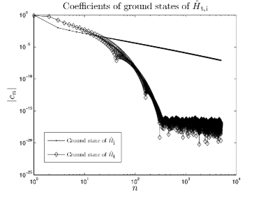
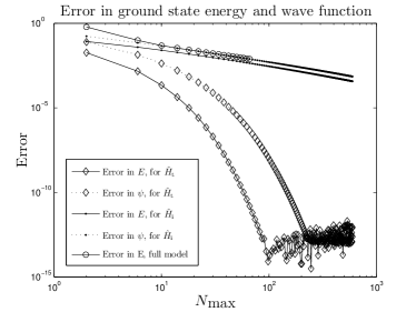
Figure 4: Left: Coefficients of the exact ground states of the Hamiltonians $\hat{H}_{\text{t,i}}$. For $\hat{H}_{\text{i}}$ only even-numbered coefficients are nonzero and thus displayed. The almost straight line indicates approximately $o(n^{-1.57})$ decay of the coefficients around $n=600$ and $o(n^{-1.73})$ around $n=5000$. Compare with Fig. 2. For the $\hat{H}_{\text{t}}$ ground state we clearly have spectral convergence. Right: The error in the ground state energies and wave functions when using the CI method. For $\hat{H}_{\text{i}}$ we have $o(n^{-1.24})$ decay for the energy error, and $o(n^{-1.20})$ decay for the wave function error, both evaluated at $n=600$. For $\hat{H}_{\text{t}}$ we clearly have spectral convergence. A full two-particle CI calculation is superimposed, showing that the error in the interaction part of the Hamiltonian (2) completely dominates. Here, the error in the energy is $o(N_{\text{max}}^{-1.02})$ at $n=70$, while for $\hat{H}_{\text{i}}$ alone, we have $o(N_{\text{max}}^{-1.01})$.

We could overcome this problem by choosing a different set of basis functions for the Hilbert space, and thus a different model space $\mathcal{P}$ altogether. However, the symmetries of the h.o. lets us treat the interaction potential with ease by explicitly performing the centre-of-mass transformation, a significant advantage in many-body calculations. In our one-dimensional case, we could replace $U(x_{1}-x_{2})$ by a smooth potential; after all $U$ is just an approximation somewhat randomly chosen. We would then obtain much better results with the CI method. However, we are not willing to trade the bare Coulomb interaction in two (or even three) dimensions for an approximation. After all we know that the singular and long-range nature of the interaction is essential.

We therefore propose to use effective interaction theory known from many-body physics to improve the accuray of CI calculations for quantum dots. This replaces the matrix in the h.o. basis of the interaction term with an approximation, giving exact eigenvalues in the case of no trap perturbation $v(x)$, regardless of the energy cut parameter $N_{\text{max}}$. We cannot hope to gain spectral convergence; the eigenfunctions are still non-smooth. However, we can increase the algebraic convergence considerably by modifying the interaction matrix for the given model space. This is explained in detail in the next section.

IV Effective Hamiltonian theory

IV.1 Similarity transformation approach

The theories of effective interactions have been, and still are, vital ingredients in many-body physics, from quantum chemistry to nuclear physics.Helgaker et al. (2000); Lindgren and Morrison (1985); Hjorth-Jensen et al. (1995); Dickhoff and Neck (2005); Blaizot and Ripka (1986); Caurier et al. (2005) In fields like nuclear physics, due to the complicated nature of the nuclear interactions, no exact spatial potential exists for the interactions between nucleons. Computation of the matrix elements of the many-body Hamiltonian then amounts to computing, for example, successively complicated Feynman diagrams,Hjorth-Jensen et al. (1995); Dickhoff and Neck (2005) motivating realistic yet tractable approximations such as effective two-body interactions. These effective interactions are in turn used as starting points for diagonalization calculations in selected model spaces.Caurier et al. (2005); Navrátil and Barrett (1998); Navrátil et al. (2000, 2000) Alternatively, they can be used as starting point for the resummation of selected many-body correlations such as in coupled-cluster theories.Helgaker et al. (2000) In our case, it is the so-called curse of dimensionality that makes a direct approach unfeasible: The number of h.o. states needed to generate accurate energies and wave functions grows exponentially with the number of particles in the system. Indeed, the dimension of $\mathcal{P}$ grows as $N_{\text{max}}^{Nd}/(Nd)!$

For the derivation of the effective interaction, we consider the Hamiltonian (2) in centre-of-mass coordinates, i.e.,

$$\hat{H} = \hat{h}(X)+\hat{h}(x)+v\big{(}(X+x)/\sqrt{2}\big{)}+$$

$$v\big{(}(X-x)/\sqrt{2}\big{)}+U(\sqrt{2}x;\lambda,\delta).$$

For $v(x)\neq 0$, the Hamiltonian is clearly not separable. The idea is then to treat $v(x_{j})$ as perturbations of a system separable in centre-of-mass coordinates; after all the trap potential is assumed to be smooth. This new unperturbed Hamiltonian reads

$$\hat{H}^{\prime}=\hat{h}(X)+\hat{h}(x)+\hat{V},$$

where $\hat{V}=U(\sqrt{2}x;\lambda,\delta)$, or any other interaction in a more general setting. We wish to replace the CI matrix of $\hat{H}^{\prime}$ with a different matrix $\hat{H}^{\prime}_{\text{eff}}$, having the exact eigenvalues of $\hat{H}^{\prime}$, but necessarily only approximate eigenvectors.

The effective Hamiltonian $\hat{H}^{\prime}_{\text{eff}}$ can be viewed as an operator acting in the model space while embodying information about the original interaction in the complete space $\mathcal{H}$. We know that this otherwise neglected part of Hilbert space is very important if $\hat{V}$ is not small. Thus, the first ingredient is the splitting of the Hilbert space into the model space $\mathcal{P}=P\mathcal{H}$ and the excluded space $\mathcal{Q}=Q\mathcal{H}=(1-P)\mathcal{H}$. Here, $P$ is the orthogonal projector onto the model space.

In the following, we let $N$ be the dimension of the model space $\mathcal{P}$. There should be no danger of confusion with the number of particles $N=2$, as this is now fixed. Moreover, we let $\{\Phi_{n}\}_{n=1}^{N}$ be an orthonormal basis for $\mathcal{P}$, and $\{\Phi_{n}\}_{n=N+1}^{\infty}$ be an orthonormal basis for $\mathcal{Q}$.

The second ingredient is a decoupling operator $\omega$. It is an operator defined by the properties

$$P\omega=\omega Q=0,$$

which essentially means that $\omega$ is a mapping from the model space to the excluded space. Indeed,

$$\omega = (P+Q)\omega(P+Q)=P\omega P+P\omega Q+Q\omega P+Q\omega Q$$

$$= Q\omega P,$$

which shows that the kernel of $\omega$ includes $\mathcal{Q}$, while the range of $\omega$ excludes $\mathcal{P}$, i.e., that $\omega$ acts only on states in $\mathcal{P}$ and yields only states in $\mathcal{Q}$.

The effective Hamiltonian $\hat{H}_{\text{eff}}=P[\hat{h}(x)+\hat{h}(X)]P+\hat{V}_{\text{eff}}$, where $\hat{V}_{\text{eff}}$ is the effective interaction, is given by the similarity transformationSuzuki and Okamoto (1994)

$$\hat{H}_{\text{eff}}=Pe^{-z}\hat{H}e^{z}P,$$ (11)

where $z=\operatorname{artanh}(\omega-\omega^{\dagger})$. The key point is that $e^{z}$ is a unitary operator with $(e^{z})^{-1}=e^{-z}$, so that the $N$ eigenvalues of $\hat{H}^{\prime}_{\text{eff}}$ are actually eigenvalues of $\hat{H}^{\prime}$.

In order to generate a well-defined effective Hamiltonian, we must define $\omega=Q\omega P$ properly. The approach of Suzuki and collaboratorsSuzuki (1982); suz ; Suzuki and Okamoto (1995, 1994) is simple: Select an orthonormal set of vectors $\{\chi_{n}\}_{n=1}^{N}$. These can be some eigenvectors of $\hat{H}^{\prime}$ we wish to include. Assume that $\{P\chi_{n}\}_{n=1}^{N}$ is a basis for the model space, i.e., that for any $n\leq N$ we can write

$$\Phi_{n}=\sum_{m=1}^{N}a_{n,m}P\chi_{m}$$

for some constants $a_{n,m}$. We then define $\omega$ by

$$\omega P\chi_{n}:=Q\chi_{n},\quad n=1,\ldots,N.$$

Observe that $\omega$ defined in this way is an operator that reconstructs the excluded space components of $\chi_{n}$ given its model space components, thereby indeed embodying information about the Hamiltonian acting on the excluded space.

Using the decoupling properties of $\omega$ we quickly calculate

$$\omega\Phi_{n}=Q\omega P\Phi_{n}=Q\omega\sum_{m=1}^{N}a_{n,m}\chi_{m},\quad n=1,\ldots,N$$

and hence for any $n^{\prime}>N$ we have

$$\langle\Phi_{n^{\prime}},\omega\Phi_{n}\rangle=\sum_{m=1}^{N}a_{n,m}\langle\Phi_{n^{\prime}},\chi_{m}\rangle,$$

yielding all the non-zero matrix elements of $\omega$.

As for the vectors $\chi_{n}$, we do not know a priori the exact eigenfunctions of $\hat{H}^{\prime}$, of course. Hence, we cannot find $\hat{H}^{\prime}_{\text{eff}}$ exactly. The usual way to find the eigenvalues is to solve a much larger problem with $N^{\prime}>N$ and then assume that these eigenvalues are “exact”. The reason why this is possible at all is that our Hamiltonian $\hat{H}^{\prime}$ is separable, and therefore easier to solve. However, we have seen that this is a bad method: Indeed, one needs a matrix dimension of about $10^{10}$ to obtain about 10 significant digits. Therefore we instead reuse the aforementioned constant reference potential method to obtain eigenfunctions and eigenvectors accurate to machine precision.

Which eigenvectors of $\hat{H}^{\prime}$ do we wish to include? Intuitively, the first choice would be the lowest $N$ eigenvectors. However, simply ordering the eigenvalues “by value” is not what we want here. Observe that $\hat{H}^{\prime}$ is block diagonal, and that the model space contains $N_{\text{max}}+1$ blocks of sizes 1 through $N_{\text{max}}+1$. If we look at the exact eigenvalues, we know that they have the structure

$$E_{n,m}=(n+1/2)+\epsilon_{m},$$

where $n$ is the block number and $\epsilon_{m}$ are the eigenvalues of $\hat{H}_{\text{i}}$, see Eq. (4). But it is easy to see that the large-scale diagonalization eigenvalues do not have this structure – we only obtain this in the limit $N_{\text{max}}\rightarrow\infty$. Therefore we choose the eigenvectors corresponding to the $N$ eigenvalues $E_{n,m}$, $n+m\leq N_{\text{max}}$, thereby achieving this structure in the eigenvalues of $\hat{H}^{\prime}_{\text{eff}}$.

In general, we wish to incorporate the symmetries of $\hat{H}^{\prime}$ into the effective Hamiltonian $\hat{H}^{\prime}_{\text{eff}}$. In this case, it was the separability and even eigenvalue spacing we wished to reproduce. In Sec. V we treat the two-dimensional Coulomb problem similarly.

IV.2 Numerical experiments with effective interactions

The eigenvectors of the Hamiltonian $\hat{H}^{\prime}$ differ from those of the the effective Hamiltonian $\hat{H}^{\prime}_{\text{eff}}$. In this section, we first make a qualitative comparison between the ground states of each Hamiltonian. We then turn to a numerical study of the error in the CI method when using the effective interaction in a the model problem.

Recall that the ground state eigenvectors are on the form

$$\Psi(X,x)=\phi_{0}(X)\psi(x)=\phi_{0}(X)\sum_{n=0}^{\infty}c_{n}\phi_{n}(x).$$

For $\hat{H}^{\prime}_{\text{eff}}$, $c_{n}=0$ for all $n>N_{\text{max}}$, so that the excluded space-part of the error concides with the excluded space-part of the exact ground state. In Fig. 5 the coefficients $c_{n}$ for both $\hat{H}^{\prime}$ and $\hat{H}^{\prime}_{\text{eff}}$ are displayed. The pointwise error is also plotted, and the largest values are seen to be around $x=0$. This is expected since $U(\sqrt{2}x;\lambda,\delta)$ and the exact ground state is non-smooth there. Notice the slow spatial decay of the error, intuitively explained by the slow decay of the Coulomb interaction.

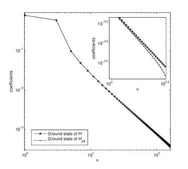
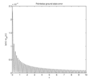
Figure 5: Left: Plot of ground state coefficients of $\hat{H}^{\prime}$ and $\hat{H}_{\text{eff}}$. Right: Pointwise error (in relative coordinate $x$) of effective Hamiltonian ground state $\psi_{\text{eff}}(x)$

We now turn to a simulation of the full two-particle Hamiltonian (2), and compare the decay of the ground state energy error with and without the effective interaction. Thus, we perform two simulations with Hamiltonians

$$\hat{H} = \hat{H}^{\prime}+v(x_{1})+v(x_{2})$$

$$= \hat{h}(x_{1})+\hat{h}(x_{2})+v(x_{1})+v(x_{2})+\hat{T}\hat{V}\hat{T}^{\dagger}$$

and

$$\hat{H}_{\text{eff}} = \hat{H}^{\prime}_{\text{eff}}+v(x_{1})+v(x_{2})$$

$$= \hat{h}(x_{1})+\hat{h}(x_{2})+v(x_{1})+v(x_{2})+\hat{T}\hat{V}_{\text{eff}}\hat{T}^{\dagger},$$

respectively, where $\hat{T}$ is the centre-of-mass transformation, cf. Eq. (7).

We remark that the new Hamiltonian matrix has the same structure as the original matrix. It is only the values of the interaction matrix elements that are changed. Hence, the new scheme has the same complexity as the CI method if we disregard the computation of $\hat{V}_{\text{eff}}$, which is a one-time calculation of low complexity.

The results are striking: In Fig. 6 we see that the ground state error decays as $O(N_{\text{max}}^{-2.57})$, compared to $O(N_{\text{max}}^{-0.95})$ for the original CI method. For $N_{\text{max}}=40$, the CI relative error is $\Delta E/E_{0}\approx 2.6\cdot 10^{-3}$, while for the effective interaction approach $\Delta E/E_{0}\approx 1.0\cdot 10^{-5}$, a considerable gain.

The ground state energy $E_{0}$ used for computing the errors were computed using extrapolation of the results.

We comment that $N_{\text{max}}\sim 40$ is the practical limit on a single desktop computer for a two-dimensional two-particle simulation. Adding more particles further restricts this limit, emphasizing the importance of the gain achieved in the relative error.

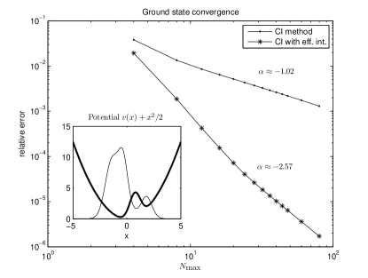
Figure 6: Ground state energy relative error for a two-particle simulation using the confinement potential $V(x)=x^{2}/2+4\exp(-2(x-0.75)^{2})$. For the CI method without effective interactions, we obtain $\alpha\approx-1.02$, while the effective interactions gives $\alpha\approx-2.57$. The electron density is superimposed on the potential plot.

In a more systematical treatment, we computed the error decay coefficient $\alpha$ for a range of trap potentials $x^{2}+A\exp(-2(x-\mu)^{2})$, where we vary $A$ and $\mu$ to create single and double-well potentials. In most cases we could estimate $\alpha$ successfully. For low values of $\mu$, i.e., near-symmetric wells, the parameter estimation was difficult in the effective interaction case due to very quick convergence of the energy. The CI calculations also converged quicker in this case. Intuitively this is so because the two electrons are far apart in this configuration.

The results indicate that at $N_{\text{max}}=60$ we have

$$\alpha=-0.96\pm 0.04\quad\text{for $\hat{H}$}$$

and

$$\alpha=-2.6\pm 0.2\quad\text{for $\hat{H}_{\text{eff}}$}$$

for the chosen model. Here, $0.6\leq\mu\leq 1.8$ and $2.9\leq A\leq 4.7$ and all the fits were successful. In Fig. 7 contour plots of the obtained results are shown. For the shown range, results were unambiguous.

These numerical results clearly indicate that the effective interaction approach will gain valuable numerical precision over the original CI method in general; in fact we have gained nearly two orders of magnitude in the decay rate of the error.

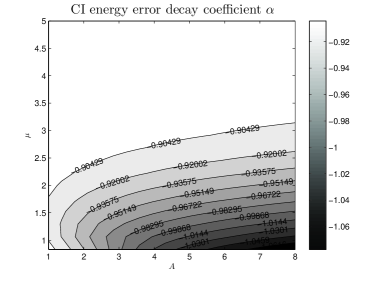
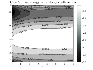
Figure 7: Estimates of $\alpha$ for CI calcilations with (right) and without (left) effective interactions.

V Discussion and outlook

V.1 Generalizations

One-dimensional quantum dot models are of limited value in themselves. However, as claimed in the Introduction, the analysis and experiments performed in this article are valid also in higher-dimensional systems.

Consider two particles in two dimensions. Let $\hat{h}(\vec{r})$ be the two-dimensional harmonic oscillator Hamiltonian (we omit the superscript in Eq. (5) for brevity), and let the quantum dot Hamiltonian be given by

$$\hat{H}=\hat{H}^{\prime}+v(\vec{r}_{1})+v(\vec{r}_{2}),$$

where

$$\hat{H}^{\prime}=\hat{h}(\vec{r}_{1})+\hat{h}(\vec{r}_{2})+\frac{\lambda}{\|\vec{r}_{1}-\vec{r}_{2}\|}.$$

The normalized centre-of-mass and relative coordinates are defined by

$$\vec{R}=\frac{\vec{r}_{1}+\vec{r}_{2}}{\sqrt{2}}\quad\text{and}\quad\vec{r}=\frac{\vec{r}_{1}-\vec{r}_{2}}{\sqrt{2}},$$

respectively, which gives

$$\hat{H}^{\prime}=\hat{h}(\vec{R})+\hat{h}(\vec{r})+\frac{\lambda}{\sqrt{2}\|\vec{r}\|}.$$

The h.o. eigenfunctions in polar coordinates are given byRontani et al. (2006)

$$\Phi_{n,m}(r,\theta)\propto e^{im\theta}r^{|m|}L_{n}^{|m|}(r^{2})e^{-r^{2}/2},$$

and the corresponding eigenvalues are $2n+|m|+1$. Now, $\hat{H}^{\prime}$ is further separable in polar coordinates, yielding a single radial eigenvalue equation to solve, analoguous to the single one-dimensional eigenvalue equation of $\hat{H}_{\text{i}}$ in Eq. (4).

The eigenvalues of $\hat{H}^{\prime}$ have the structure

$$E_{n^{\prime},m^{\prime},n,m}=2n^{\prime}+|m^{\prime}|+1+\epsilon_{n,m},$$

where $(n^{\prime},m^{\prime})$ and $(n,m)$ are the centre-of-mass and relative coordinate quantum numbers, respectively. Again, the degeneracy structure and even spacing of the eigenvalues are destroyed in the CI approach, and we wish to regain it with the effective interaction. We then choose the eigenvectors corresponding to the quantum numbers

$$2n^{\prime}+|m^{\prime}|+2n+m\leq N_{\text{max}}$$

to build our effective Hamiltonian $\hat{H}^{\prime}_{\text{eff}}$.

Let us also mention, that the exact eigenvectors $\Psi_{n^{\prime},m^{\prime},n,m}$ are non-smooth due to the $1/r$-singularity of the Coulomb interaction. The approximation properties of the Hermite functions are then directly applicable as before, when we expand the eigenfunctions in h.o. basis functions. Hence, the configuration-interaction method will converge slowly also in the two-dimensional case. It is good reason to believe that effective interaction experiments will yield similarly positive results with respect to convergence improvement.

Clearly, the above procedure is applicable to three-dimensional problems as well. The operator $\hat{H}^{\prime}$ is separable and we obtain a single non-trivial radial equation, and thus we may apply our effective Hamiltonian procedure. The exact eigenvalues will have the structure

$$E_{n^{\prime},l^{\prime},m^{\prime},n,l,m}=2n^{\prime}+l^{\prime}+\frac{3}{2}+\epsilon_{n,l,m},$$

on which we base the choice of the effective Hamiltonian eigenvectors as before.

The effective interaction approach to the configuration-interaction calculations is easily extended to a many-particle problem, whose Hamiltonian is given by Eq. (1). The form of the Hamiltonian contains only interactions between pairs of particles, and $\hat{V}_{\text{eff}}$ as defined in Sec. IV can simply replace these terms.

V.2 Outlook

A theoretical understanding of the behavior of many-body systems is a great challenge and provides fundamental insights into quantum mechanical studies, as well as offering potential areas of applications. However, apart from some few analytically solvable problems, the typical absence of an exactly solvable contribution to the many-particle Hamiltonian means that we need reliable numerical many-body methods. These methods should allow for controlled expansions and provide a calculational scheme which accounts for successive many-body corrections in a systematic way. Typical examples of popular many-body methods are coupled-cluster methods,Bartlett (1981); Helgaker et al. (2000); Wloch et al. (2005) various types of Monte Carlo methods,Pudliner et al. (1997); Ceperley (1995); mc (3) perturbative expansions,Lindgren and Morrison (1985); Hjorth-Jensen et al. (1995) Green’s function methods,Dickhoff and Neck (2005); Blaizot and Ripka (1986) the density-matrix renormalization groupWhite (1992); Schollwock (2005) and large-scale diagonalization methods such as the CI method considered here.

In a forthcoming article, we will apply the similarity transformed effective interaction theory to a two-dimensional system, and also extend the results to many-body situations. Application of other methods, such as coupled-cluster calculations, are also an interesting approach, and can give further refinements on the convergence, as well as gaining insight into the behaviour of the numerical methods in general.

The study of this effective Hamiltonian is interesting from a many-body point of view: The effective two-body force is built from a two-particle system. The effective two-body interaction derived from an $N$-body system, however, is not necessarly the same. Intuitively, one can think of the former approach as neglecting interactions and scattering between three or more two particles at a time. In nuclear physics, such three-body correlations are non-negligible and improve the convergence in terms of the number of harmonic oscillator shells.Navrátil and Ormand (2003) Our hope is that such interactions are much less important for Coulomb systems.

Moreover, as mentioned in the Introduction, accurate determination of eigenvalues is essential for simulations of quantum dots in the time domain. Armed with the accuracy provided by the effective interactions, we may commence interesting studies of quantum dots interacting with their environment.

V.3 Conclusion

We have mathematically and numerically investigated the properties of the configuration-interaction method, or “exact diagonalization method”, by using results from the theory of Hermite series. The importance of the properties of the trap and interaction potentials is stressed: Non-smooth potentials severely hampers the numerical properties of the method, while smooth potentials yields exact results with reasonable computing resources. On the other hand, the h.o. basis is very well suited due to the symmetries under orthogonal coordinate changes.

In our numerical experiments, we have demonstrated that for a simple one-dimensional quantum dot with a smooth trap, the use of similarity transformed effective interactions can significantly reduce the error in the configuration-interaction calculations due to the non-smooth interaction, while not increasing the complexity of the algorithm. This error reduction can be crucial for many-body simulations, for which the number of harmonic oscillator shells is very modest.

References

- Helgaker et al. (2000) T. Helgaker, P. Jørgensen, and J. Olsen, Molecular Electronic Structure Theory. Energy and Wave Functions (Wiley, New York, USA, 2000).
- Caurier et al. (2005) E. Caurier, G. Martinez-Pinedo, F. Nowacki, A. Poves, and A. P. Zuker, Rev. Mod. Phys. 77, 427 (2005),
- Ezaki et al. (1997) T. Ezaki, N. Mori, and C. Hamaguchi, Phys. Rev. B 56, 6428 (1997).
- Maksym (1998) P. Maksym, Physica B 249, 233 (1998).
- Bruce and Maksym (2000) N. A. Bruce and P. A. Maksym, Phys. Rev. B 61, 4718 (2000).
- Creffield et al. (1999) C. E. Creffield, W. Häusler, J. H. Jefferson, and S. Sarkar, Phys. Rev. B 59, 10719 (1999).
- Häusler and Kramer (1993) W. Häusler and B. Kramer, Phys. Rev. B 47, 16353 (1993).
- Reimann et al. (2000) S. M. Reimann, M. Koskinen, and M. Manninen, Phys. Rev. B 62, 8108 (2000).
- Rontani et al. (2006) M. Rontani, C. Cavazzoni, D. Belucci, and G. Goldoni, J. Chem. Phys. 124, 124102 (2006).
- Ciftja and Faruk (2006) O. Ciftja and M. G. Faruk, J. Phys.: Condens. Mat. 18, 2623 (2006).
- Jauregui et al. (1993) K. Jauregui, W. Hausler, and B. Kramer, Europhys. Lett. 24, 581 (1993).
- Imamura et al. (1999) H. Imamura, P. A. Maksym, and H. Aoki, Phys. Rev. B 59, 5817 (1999).
- Tavernier et al. (2003) M. B. Tavernier, E. Anisimovas, F. M. Peeters, B. Szafran, J. Adamowski, and S. Bednarek, Phys. Rev. B 68, 205305 (2003).
- Wensauer et al. (2004) A. Wensauer, M. Korkusinski, and P. Hawrylak, Solid State Communications 130, 115 (2004).
- Helle et al. (2005) M. Helle, A. Harju, and R. M. Nieminen, Phys. Rev. B 72, 205329 (2005).
- Xie (2006) W. Xie, Phys. Rev. B 74, 115305 (2006).
- Tavernier et al. (2006) M. B. Tavernier, E. Anisimovas, and F. M. Peeters, Phys. Rev. B 74, 125305 (2006).
- Gylfadottir et al. (2006) S. S. Gylfadottir, A. Harju, T. Jouttenus, and C. Webb, New Journal of Physics 8, 211 (2006).
- Gould (1995) S. Gould, Variational Methods for Eigenvalue Problems: An Introduction to the Methods of Rayleigh, Ritz, Weinstein, and Aronszajn (Dover, New York, USA, 1995).
- Tang (1993) T. Tang, SIAM Journal on Scientific Computing 14, 594 (1993).
- Navrátil and Barrett (1998) P. Navrátil and B. R. Barrett, Phys. Rev. C 57, 562 (1998).
- Navrátil et al. (2000) P. Navrátil, J.P. Vary, and B.R. Barrett, Phys. Rev. Lett. 84, 5728 (2000).
- Navrátil et al. (2000) P. Navrátil, G. P. Kamuntavicius, and B. R. Barrett, Phys. Rev. C 61, 44001 (2000).
- Suzuki (1982) K. Suzuki, Prog. Theor. Phys. 68, 246 (1982).
- (25) K. Suzuki, Prog. Theor. Phys. 68, 1627 (1982); K. Suzuki and R. Okamoto, ibid. 75, 1388 (1986); 76, 127 (1986).
- Suzuki and Okamoto (1995) K. Suzuki and R. Okamoto, Prog. Theor. Phys. 93, 905 (1995).
- Suzuki and Okamoto (1994) K. Suzuki and R. Okamoto, Prog. Theor. Phys. 92, 1045 (1994).
- Kamada et al. (2001) H. Kamada, A. Nogga, W. Glockle, E. Hiyama, M. Kamimura, K. Varga, Y. Suzuki, M. Viviani, A. Kievsky, S. Rosati, et al., Phys. Rev. C 64, 044001 (2001).
- Varga et al. (2001) K. Varga, P. Navrátil, J. Usukura, and Y. Suzuki, Phys. Rev. B 63, 205308 (2001).
- Loss and DiVincenzo (1998) D. Loss and D. P. DiVincenzo, Phys. Rev. A 57, 120 (1998).
- Boyd (1984) J. Boyd, J. Comp. Phys. 54, 382 (1984).
- Hille (1939) E. Hille, Duke Math. J. 5, 875 (1939).
- Kumar et al. (1990) A. Kumar, S.E. Laux, and F. Stern, Phys. Rev. B 42, 5166 (1990).
- Macucci et al. (1997) M. Macucci, K. Hess, and G. J. Iafrate, Phys. Rev. B 55, R4879 (1997).
- Maksym and Bruce (1997) P. A. Maksym and N. A. Bruce, Physica E 1, 211 (1997).
- Wensauer et al. (2003) A. Wensauer, M. Korkusinski, and P. Hawrylak, Phys. Rev. B 67, 035325 (2003).
- Kurasov (1996) P. Kurasov, J. Phys. A: Math. Gen. 29, 1767 (1996).
- Gesztesy (1980) F. Gesztesy, J. Phys. A: Math. Gen. 13, 867 (1980).
- Tveito and Winther (2002) A. Tveito and R. Winther, Introduction to Partial Differential Equations (Springer, Berlin, Germany, 2002).
- Mota et al. (2002) R. Mota, V. D. Granados, A. Queijiro, and J. Garcia, J. Phys. A: Math. Gen. 36, 2979 (2002).
- Wensauer et al. (2000) A. Wensauer, O. Steffens, M. Suhrke, and U. Rössler, Phys. Rev. B 62, 2605 (2000).
- Harju et al. (2002) A. Harju, S. Siljamaki, and R.M. Nieminen, Phys. Rev. Lett. 88, 226804 (2002).
- Førre et al. (2006) M. Førre, J. P. Hansen, V. Popsueva, and A. Dubois, Phys. Rev. B 74, 165304 (2006).
- Ledoux et al. (2004) V. Ledoux, M. Van Daele, and G. Vanden Berghe, Comp. Phys. Comm. 162, 151 (2004).
- Ledoux et al. (2005) V. Ledoux, M. Van Daele, and G. Vanden Berghe, ACM T. Math. Software 31, 532 (2005).
- Lindgren and Morrison (1985) I. Lindgren and J. Morrison, Atomic Many-Body Theory (Springer, Berlin, Germany, 1985).
- Hjorth-Jensen et al. (1995) M. Hjorth-Jensen, T. T. S. Kuo, and E. Osnes, Phys. Rep. 261, 125 (1995).
- Dickhoff and Neck (2005) W. H. Dickhoff and D. V. Neck, Many-Body Theory exposed! (World Scientific, New Jersey, USA, 2005).
- Blaizot and Ripka (1986) J. P. Blaizot and G. Ripka, Quantum theory of finite systems (MIT press, Cambridge, USA, 1986).
- Bartlett (1981) R. J. Bartlett, Ann. Rev. Phys. Chem. 32, 359 (1981).
- Pudliner et al. (1997) B. S. Pudliner, V. R. Pandharipande, J. Carlson, S. C. Pieper, and R. B. Wiringa, Phys. Rev. C 56, 1720 (1997).
- Ceperley (1995) D. M. Ceperley, Rev. Mod. Phys. 67, 279 (1995).
- mc (3) S. E. Koonin, D. J. Dean, and K. Langanke, Phys. Rep. 278, 1 (1997); T. Otsuka, M. Homna, T. Mizusaki, N. Shimizu, and Y. Utsuno, Prog. Part. Nucl. Part. 47, 319 (2001).
- White (1992) S. R. White, Phys. Rev. Lett. 69, 2863 (1992).
- Schollwock (2005) U. Schollwock, Rev. Mod. Phys. 77, 259 (2005).
- Navrátil and Ormand (2003) P. Navrátil and W. E. Ormand, Phys. Rev. C 68, 034305 (2003).
- Wloch et al. (2005) M. Wloch, D. J. Dean, J. R. Gour, M. Hjorth-Jensen, K. Kowalski, T. Papenbrock, and P. Piecuch, Phys. Rev. Lett. 94, 212501 (2005).