Cooling of a Micro-mechanical Resonator by the Back-action of Lorentz Force

Abstract

Using a semi-classical approach, we describe an on-chip cooling protocol for a micro-mechanical resonator by employing a superconducting flux qubit. A Lorentz force, generated by the passive back-action of the resonator’s displacement, can cool down the thermal motion of the mechanical resonator by applying an appropriate microwave drive to the qubit. We show that this on-chip cooling protocol, with well-controlled cooling power and a tunable response time of passive back-action, can be highly efficient. With feasible experimental parameters, the effective mode temperature of a resonator could be cooled down by several orders of magnitude.

I Introduction

The rapid development of nano-technology has enabled fabrication of micro or nano-mechanical resonator Cleland (2002); Blencowe (2004) with high frequency, low dissipation and small mass. In the way to observe quantized mechanical motion LaHaye et al. (2004), thermal fluctuation has become a major obstacles. The limited cooling efficiency and poor heat conduction at the milli-Kelvin temperatures of cryogenic refrigerators has stimulated a number of studies on the active cooling of micromechanical resonator (MR) in both classical regime and quantum regimes Cohadon et al. (1999); Kleckner and Bouwmeester (2006); Poggio et al. (2007); Metzger and Karrai (2004); Gigan et al. (2006); Arcizet et al. (2006); Schliesser et al. (2006); Naik et al. (2006); Hopkin et al. (2003); Wilson-Rae et al. (2004); Martin et al. (2004); Zhang et al. (2005); Brown et al. (2007); Xue et al. (2007a); Corbitt et al. (2007); Thompson et al. (2007); Mow-Lowry et al. (2008); You et al. (2008). Of these proposals, the optomechanical cooling is the most highly developed one experimentally. For example, it has been successfully used to demonstrate cooling Thompson et al. (2007); Poggio et al. (2007) from room temperature down to $6.82$ mK and from $2.2$ K down to $2.9$ mK. Optomechanical cooling has also been studied theoretically in the quantum limit Marquardt et al. (2007); Genes et al. (2007); Wilson-Rae et al. (2007).

In a thermal environment, a MR randomly vibrates around its equilibrium position due to thermal fluctuation. The effective temperature of a MR mode can be defined by the mean kinetic energy of this mode. Cooling of MR is equivalent to suppressing the mean amplitude of the Brownian motion, which is the major barrier to precise displacement measurement. The optomechanical cooling of an MR is achieved by the passive back-action or active feedback of such optical forces as bolometric force Braginsky and Vyatchanin (2002); Metzger and Karrai (2004) and radiation pressure  Cohadon et al. (1999); Kleckner and Bouwmeester (2006); Poggio et al. (2007); Gigan et al. (2006); Arcizet et al. (2006); Schliesser et al. (2006) from a laser driven optical cavity.

Instead of employing an optical component, in this paper, we present a cooling protocol for an MR in an on-chip superconducting circuit containing three or four Josephson junctions (JJ). The three-junction superconducting loop forms a flux qubit Mooij et al. (1999); Orlando et al. (1999); Wilhelm and Semba (2006). The typical energy scale of the Larmor frequency of the flux qubit is normally several GHz which is much larger than the oscillation frequency of the MR studied in this paper. The persistent current in this loop exerts a Lorentz force on an MR under an in-plane magnetic field Xue et al. (2007b); Gaidarzhy et al. (2005). This circulating superconducting current is modulated by the thermal motion of the MR through nonlinear Josephson inductance in a delayed way. Thus the Lorentz force exerted on the MR depends on the motion of the MR itself. This force acts as a passive back-action on the MR as the radiation pressure in the optomechanical cooling strategy. The thermal motion of the MR is damped by this back-action force with appropriate parameters. To use a microwave bias to drive the superconducting circuit helps to take away the thermal energy of the resonator. In other words, in the linear response regime, a microwave drive together with a flux qubit in a dissipative environment can be treated as an effective bath whose temperature is lower than that of the environmental temperature $T_{0}$. Thereby the mode temperature of the resonator, which is proportional to the mean kinetic energy of the fundamental oscillation mode, is decreased Martin et al. (2004); Clerk and Bennett (2005); Blencowe et al. (2005). The strong and tunable coupling between superconducting current and the MR displacement is favorable as regards obtaining highly-efficient and well-controlled cooling. Based on feasible experimental parameters, we also provide a detailed analysis of the cooling efficiency of this scheme. The estimation shows that it could constitute a promising alternative to optomechanical cooling.

This paper is organized as follows: In Sec. II, we describe the setup we use to implement our cooling scheme. Sec. III presents the intuitive picture of this back-action cooling by Lorentz force, together with a general formalism for dealing with self back-action cooling. In Sec. IV, the cooling efficiency of this physical system is determined based on a detailed calculation of the ”spring constant” and the response time of the Lorentz force. The lengthy calculation part concerning to the master equation and its steady-state solution are given in the Appendix. In Sec. V, cooling efficiency is estimated by using feasible experimental parameters . Finally in Sec. VI, we discuss the possible advantages, fluctuation and measurement protocol of this cooling protocol.

II The Setup

A schematic diagram of the setup for this cooling protocol is shown in Fig.1.

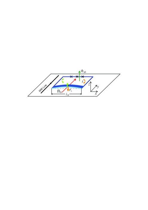
Figure 1: (Color on line) Schematic diagram of our setup. A doubly-clamped mechanical beam is incorporated in a superconducting loop with a superconducting Josephson junction (indicated with crosses) flux qubit. The initial bias in the loop is controlled by magnetic flux $\Phi_{z0}$ in $z$ direction. A coupling magnetic field $B_{0}$ is imposed on the beam in the $y$ direction and the supercurrent under this magnetic field imposes a Lorentz force on the beam. A microwave line introduces a microwave bias to the qubit loop. The magnitude of the Lorentz force depends on the motion of the beam through the change of the supercurrent in the loop in a delayed way. This delayed back-action damps the motion of the beam in the $z$ direction and thereby cools down the thermal motion of the beam.

In the $x$-$y$ plane, a doubly-clamped micro-mechanical beam with an effective length $L_{0}$ is incorporated in a superconducting loop with three small-capacitance Josephson junctions. This mechanical beam can be created from a surface-micromachined silicon or carbon nanotube Poncharal et al. (1999) coated with superconducting material, or a self-supporting metallic airbridge. The fundamental vibration mode of the beam can be well approximated by using a harmonic resonator with oscillation frequency $\omega_{b}$. With a proper bias magnetic flux, two classical stable states of the 3-JJ loop carry persistent currents in opposite directions. There is a finite tunneling rate $\Delta$ between the two classical persistent-current states (throughout this article, we let $\hbar=1$). By choosing parameters carefully, the subspace spanned by the two states is well separated from other energy levels and the superconducting loop with Josephson junctions forms a two-level system (superconducting flux qubit) Mooij et al. (1999); Orlando et al. (1999) and coherent dynamics can be observed Chiorescu et al. (2003); Saito et al. (2004). Recently, the microwave-induced cooling of a flux qubit has been demonstrated experimentally Valenzuela et al. (2006) assisted by the third energy eigen-state of the three-junction superconducting loop. The qubit ground state $|g\rangle$ and excited state $|e\rangle$ are coherent superpositions of two persistent current states denoted by $|0\rangle$ (clockwise current state) and $|1\rangle$ (anti-clockwise current state). The energy spacing between the two eigenstates is $\Omega=\sqrt{\Delta^{2}+\varepsilon^{2}}$ where $\varepsilon=2I_{p}\left(\Phi_{ext}-\Phi_{0}/2\right)$ is the energy spacing of the two classical current states ($|0\rangle$ and $|1\rangle$), with $\Phi_{ext}$ the external magnetic flux through the loop, $I_{p}$ the largest persistent current in the loop and $\Phi_{0}$ the flux quantum. A microwave line is placed close to the circuit and generates microwave drive with frequency $\omega_{d}$ on the flux qubit. Under the coupling magnetic field $B_{0}$ along $y$ direction, the persistent superconducting current generates a Lorentz force $F_{L}$ on the MR along $z$ direction. This force couples the flux qubit with the oscillation motion of the MR. In the quantum regime of the MR, this configuration provides a solid-state analog of cavity QED system in strong coupling limit Xue et al. (2007b). Similar setting with a coupled MR and dc-SQUID was proposed recently to study the displacement detection and decoherence of mechanical motion Zhou and Mizel (2006); Buks and Blencowe (2006); Blencowe and Buks (2007)

In the present paper, we concentrate on a different regime where the oscillation frequency of the MR is much smaller than the Larmor frequency of the flux qubit so that the MR can be treated as a classical harmonic oscillator. Since the qubit and the MR energy scales differs greatly, the dynamics of the composite system can be handled following the line of the Born-Oppenheimer approximation: The master equation of the qubit is established by assuming a certain MR displacement $z$; the steady-state solution for the qubit dynamics is inserted into the classical Langevin equation of the MR to derive the noise spectrum of the mechanical displacement.

III The cooling mechanism

In this section, we first present an intuitive understanding of the cooling protocol based on the Lorentz force back-action. Using the classical Langevin equation of the MR, we then proceed to analyze how this back-action leads to the suppression of the random motion of the MR. The explicit form of the Lorentz force back-action in the Langevin equation will be derived in the next section.

The composite flux qubit and MR system is kept at an environmental temperature $T_{0}$ in a dilution refrigerator. The initial constant bias flux of the loop is $\Phi_{z0}$ in the $z$ direction. When the MR is displaced to $z(t)$ by thermal noise, the total magnetic flux in the superconducting loop is changed to $\Phi_{z0}+B_{0}L_{0}z(t)$. In principle, for an MR with an aspect ratio close to 1, thermal fluctuation also induces oscillation in the $y$ direction. However, since the magnetic field in the $z$ direction is much smaller than the coupling magnetic field $B_{0}$ in the $y$ direction, in this work we only study the motion in the $z$ direction. An increase or decrease in magnetic flux leads to a change in the persistent current $I$ in the loop after the system reaches a metastable state after a response time delay $\tau_{\text{resp}}$. Owing to the nonlinearity of Josephson junction inductance, the supercurrent in a metastable state depends on the total bias magnetic flux and hence depends on the displacement of the MR. Since the Lorentz force is proportional to the supercurrent, the Lorentz force exerted on the MR $F_{L}(t+\tau_{\text{resp}})$ depends on the displacement of the MR $z(t)$ before the time delay. This means that there exists a passive back-action mechanism for the MR: the motion of the MR leads to a delayed force on the MR itself. We found that, with a proper microwave drive (red-detuned with the qubit), this passive back-action damps the thermal motion of the MR. This cooling protocol is similar to that of the self cooling experiments based on optomechanical coupling Braginsky and Vyatchanin (2002); Metzger and Karrai (2004).

The above intuitive picture can be clearly understood by studying the MR dynamics. To accomplish this, we start by establishing an equation of motion for the MR.

The coupling term in the Hamiltonian of qubit-resonator composite system is Xue et al. (2007b)

$$H_{\text{int}}=B_{0}L_{0}\hat{I}z.$$ (1)

where $\hat{I}$ is the current operator. Then the Lorentz force on the resonator is

$$\hat{F}_{L}=-\frac{\partial H_{\text{int}}}{\partial z}=-B_{0}L_{0}\hat{I}$$ (2)

Suppose the MR is displaced at $z$, after a time delay $\tau_{\text{resp}}$, the resulting Lorentz force in the z metastable state $F_{L}^{\left(s\right)}\left(z\right)\equiv\mathrm{Tr}\left(\rho_{q}^{\left(s\right)}\left(z\right)\hat{F}_{L}\right)$ depends on $z$, where $\rho_{q}^{\left(s\right)}$ is the reduced density matrix of the qubit in a metastable state. For a small displacement $z$, the Lorentz force can be expanded to the linear order of $z$ as $F_{L}^{\left(s\right)}\left(z\right)=F_{0}+k_{L}z$ with $k_{L}$ the effective ”spring constant” of the Lorentz force. Since this force is a delayed response to the motion of the MR, its effect on the MR can be described by a delayed response function $h\left(t-t^{\prime}\right)\equiv 1-e^{-\gamma(t-t^{\prime})}$ with $\gamma=1/\tau_{\text{resp}}$. Under the Lorentz force, the equation of motion for the MR mode with mass $m$, rigidity $k=m\omega_{b}^{2}$ and an inherent damping rate $\Gamma$ is as follows Metzger and Karrai (2004)

$$m\frac{d^{2}z}{dt^{2}}+m\Gamma\frac{dz}{dt}+kz=F_{th}+\int_{0}^{t}\frac{dF_{L}^{\left(s\right)}\left[z\left(t^{\prime}\right)\right]}{dt^{\prime}}h\left(t-t^{\prime}\right)dt^{\prime},$$ (3)

where $F_{th}$ is the Brownian fluctuation force which is related to the environmental temperature $\left\langle F_{th}\left(t\right)F_{th}\left(t^{\prime}\right)\right\rangle=2k_{B}T_{0}m\Gamma\delta\left(t-t^{\prime}\right)$. The stable solution of the motion equation (3) is related to the effective mode temperature $T_{\text{eff}}$ of the MR by the equipartition theorem $k_{\text{eff}}\left\langle z^{2}\right\rangle=k_{B}T_{\text{eff}}$ where $k_{B}$ is the Boltzman constant. Then the cooling efficiency $\eta=T_{0}/T_{\text{eff}}$ can be written as

$$\eta^{-1}=\frac{\Gamma\omega_{\text{eff}}^{2}}{\pi}\int_{-\infty}^{+\infty}\frac{d\omega}{\left(\omega_{\text{eff}}^{2}-\omega^{2}\right)^{2}+\Gamma_{\text{eff}}^{2}\omega^{2}},$$ (4)

where

$$\Gamma_{\text{eff}} = \Gamma+\Gamma_{1},$$

$$\omega_{\text{eff}}^{2} = \omega_{b}^{2}\left(1-\frac{\gamma^{2}}{\omega^{2}+\gamma^{2}}\frac{k_{L}}{k}\right).$$ (5)

and

$$\Gamma_{1}=\Gamma Q_{M}\frac{\omega_{b}\gamma}{\omega^{2}+\gamma^{2}}\frac{k_{L}}{k},$$ (6)

with $Q_{M}=\omega_{b}/\Gamma$ is the quality factor of the MR. For $\left|k_{L}\right|\ll k$, the integral can be explicitly carried out as Metzger and Karrai (2004)

$$\eta=1+Q_{M}\frac{k_{L}}{k}\frac{\omega_{b}\gamma}{\omega_{b}^{2}+\gamma^{2}}.$$ (7)

From Eq.(7), it can be seen that the sign of $k_{L}$ determines whether the resonator is cooled or heated, i.e. when $k_{L}$ is positive, the Lorentz force damps the motion of the MR and the final temperature is lower than the original one, and vice versa. For a positive $k_{L}$, the cooling efficiency increases linearly with $k_{L}$. However, it should be noticed that both the linear response regime and the definition of a single-mode resonator are valid only for $k_{L}/k\ll 1$.

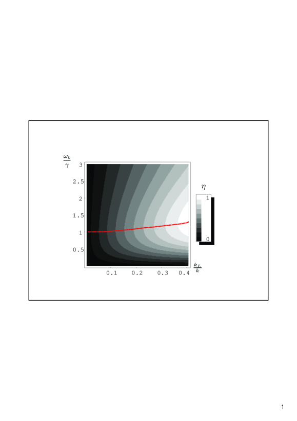
Figure 2: (Color on line) The dependence of the cooling efficiency on the ratios of $k_{L}/k$ and $\omega_{b}/\gamma$. The magnitude of the cooling efficiency is re-scaled and indicated by the gray level (higher efficiencies are shown lighter). The other parameters are the same as those used for estimating the cooling efficiency in Sec. V. The red dots indicates the point with the largest efficiency at each given $k_{L}/k$ value.

The cooling efficiency is shown by a contour plot in Fig. 2 as a function of two ratios $\omega_{b}/\gamma$ and $k_{L}/k$. $\omega_{b}/\gamma$ characterizes the ratio between the time scale of the response time and the oscillation period while $k_{L}/k$ is the scaled cooling strength of the passive Lorentz force. The magnitude of the efficiency is indicated by the gray level: Higher efficiency is represented with a lighter color. It is seen that the cooling efficiency increases with $k_{L}/k$. The strong coupling in the solid state cavity QED makes it promising to achieve larger $k_{L}$. For a given $k_{L}/k$, the largest cooling efficiency can be achieved by optimizing $\omega_{b}/\gamma$. The optimal points for each $k_{L}/k$ value are indicated by the red dots in Fig. 2. The optimal $\omega_{b}/\gamma$ slightly increases with $k_{L}$. For $k_{L}/k\ll 1$, which is in the case of interest, the red dots indicate that the optimal cooling is realized for $\omega_{b}=\gamma$. This means the largest cooling efficiency is achieved when the back-action response time matches the oscillation period of the resonator. As we show later, the response time is of the order of the relaxation time of the flux qubit. The qubit relaxation rate ranges from sub MHz to several tens of MHz, depending on the operating point $\varepsilon_{0}$ Yoshihara et al. (2006); Kakuyanagi et al. (2007), this implies that the flux qubit loop is suitable for cooling a resonator over broad frequency range. Moreover, since the operating point $\varepsilon_{0}$ can be controlled by magnetic flux $\Phi_{z0}$, the back-action response time is tunable in situ.

IV Calculation of the back-action of the Lorentz force

As we discussed in the previous section, without considering additional fluctuation, the damping effect of the Lorentz force leads to cooling or heating depending on the sign of the effective spring constant $k_{L}$: A positive $k_{L}$ leads to cooling while a negative $k_{L}$ results in heating. The cooling efficiency is proportional to the magnitude of $k_{L}$. Before proceeding with our discussion of the cooling efficiency in realistic experiment, it is necessary to obtain an explicit expression of $k_{L}$ from the dynamics of the flux qubit system.

The Lorentz force in a metastable state for a given displacement $z$ is

$$F_{L}^{\left(s\right)}\left(z\right)=-B_{0}I_{p}L_{0}\left\langle\sigma_{z}\right\rangle_{s}$$ (8)

where $\left\langle\sigma_{z}\right\rangle_{s}$ is the expectation value of $\sigma_{z}$ in a steady-state. And $\sigma_{z}$ and $\sigma_{x}$ are Pauli matrixes defined by the persistent current states as:

$$\sigma_{z}=|0\rangle\langle 0|-|1\rangle\langle 1|$$

$$\sigma_{x}=|0\rangle\langle 1|+|1\rangle\langle 0|$$ (9)

$\left\langle\sigma_{z}\right\rangle_{s}$ can be computed from the dynamics of the driven flux qubit in a dissipative environment. To do this, we start with the effective Hamiltonian of the qubit at a given displacement $z$ of the MR

$$H_{q}=\frac{\varepsilon\left(z\right)}{2}\sigma_{z}+\frac{\Delta}{2}\sigma_{x}+A\sigma_{z}\cos\omega_{d}t.$$ (10)

Here $A$ characterizes the amplitude of the microwave drive,

$$\varepsilon\left(z\right)=\varepsilon_{0}+gz$$ (11)

with $g=2B_{0}I_{p}L_{0}$, $\varepsilon_{0}=2I_{p}\Phi_{z0}$ denotes the initial bias away from the degeneracy point. If the qubit is biased at the degeneracy point, $\varepsilon_{0}=0$.

By defining a new set of Pauli operators

$$\sigma_{z}^{\prime} = \sigma_{z}\cos\theta\left(z\right)+\sigma_{x}\sin\theta\left(z\right),$$

$$\sigma_{x}^{\prime} = -\sigma_{z}\sin\theta\left(z\right)+\sigma_{x}\cos\theta\left(z\right),$$ (12)

we diagonalize the first two terms of eq.(10) as,

$$H_{q}=\frac{\Omega\left(z\right)}{2}\sigma_{z}^{\prime}+A\left(\sigma_{z}^{\prime}\cos\theta\left(z\right)-\sigma_{x}^{\prime}\sin\theta\left(z\right)\right)\cos\omega_{d}t,$$ (13)

where

$$\cos\theta\left(z\right)=\frac{\varepsilon\left(z\right)}{\Omega(z)}\ ,\ \ \sin\theta\left(z\right)=\frac{\Delta}{\Omega\left(z\right)}\ ,$$ (14)

and

$$\Omega\left(z\right)=\sqrt{\Delta^{2}+\varepsilon^{2}\left(z\right)}\approx\Omega_{0}+\tilde{g}z,$$ (15)

with $\tilde{g}=g\varepsilon_{0}/\Omega_{0}$, $\Omega_{0}=\sqrt{\Delta^{2}+\varepsilon_{0}^{2}}$ is the energy spacing between the qubit eigenstates when the displacement $z$ of the MR is zero. Here we have used the fact that the displacement $z$ is very small and $\cos\omega_{d}t$ is a fast-oscillating term.

If the drive is near-resonant with the qubit frequency $\Omega_{0}$, by performing unitary transformation $U_{R}=\exp(i\sigma_{z}^{\prime}\omega_{d}t/2)$, the Hamiltonian (13) in the rotating frame is transformed to

$$H_{R}=i\left(\frac{d}{dt}U_{R}(t)\right)U_{R}^{{\dagger}}(t)+U_{R}\left(t\right)HU_{R}^{{\dagger}}(t)=\frac{\delta\left(z\right)}{2}\sigma_{z}^{\prime}+\frac{A^{\prime}(z)}{2}\sigma_{x}^{\prime}$$ (16)

with $A^{\prime}\left(z\right)=-A\sin\theta\left(z\right)$, $\delta\left(z\right)=\delta\omega+\tilde{g}z$ and $\delta\omega=\Omega_{0}-\omega_{d}$ is the detuning between the qubit free energy and the drive. The term $A\sigma_{z}^{\prime}\cos\theta\left(z\right)\cos\omega_{d}t$ and $A\sin\theta(z)\sigma_{+}e^{i\omega_{d}t}+h.c$ in eq. (13) is neglected because $\exp(\pm i\omega_{d}t)$ and $\exp(\pm 2i\omega_{d}t)$ are fast-oscillating terms since the drive frequency is close to the qubit energy spacing. The diagonalized $H_{R}$

$$H_{R}=\frac{\omega_{0}\left(z\right)}{2}\tilde{\sigma}_{z}$$ (17)

is expressed by another set of Pauli operators

$$\tilde{\sigma}_{z} = \sigma_{z}^{\prime}\cos\beta\left(z\right)+\sigma_{x}^{\prime}\sin\beta\left(z\right),$$

$$\tilde{\sigma}_{x} = -\sigma_{z}^{\prime}\sin\beta\left(z\right)+\sigma_{x}^{\prime}\cos\beta\left(z\right),$$ (18)

with

$$\sin\beta\left(z\right)=\frac{A^{\prime}\left(z\right)}{\omega_{0}\left(z\right)},\ \ \cos\beta\left(z\right)=\frac{\delta\left(z\right)}{\omega_{0}\left(z\right)},$$ (19)

and

$$\omega_{0}\left(z\right)=\sqrt{\delta^{2}\left(z\right)+A^{\prime 2}\left(z\right)}\ .$$ (20)

With the above transformation relations, we can derive the master equation for this dissipative flux qubit in a rotating frame. Solving the master equation to obtain its steady-state solution and using the above relations to transform it back to an experimental frame, we can obtain $\langle\sigma_{z}\rangle_{s}$ in an experimental frame (see Appendix for detail)

$$\left\langle\sigma_{z}\right\rangle_{s}=\frac{2\cos^{2}\beta\left(z\right)}{1+\cos^{2}\beta\left(z\right)}\cos\theta\left(z\right)$$ (21)

From the last equation of (38), the response time needed for the supercurrent to reach this value is

$$\tau_{\text{resp}}=\frac{1}{\gamma}=\frac{1}{\Gamma_{0}}\frac{2}{1+\cos^{2}\beta_{0}}$$ (22)

with $\cos\beta_{0}\equiv\cos\beta(z=0)$. The response time is of the order of the qubit relaxation time. Shifting the qubit bias will change the qubit relaxation time and hence change the response time. On the other hand, as found with SET-assisted cooling Clerk and Bennett (2005), the response time also depends on the drive detuning and power. This is in contrast to optomechanical cooling where the response time is always determined by the cavity ring-down time.

Since $z$ is small, the force can be expanded to the linear order of $z$: $F_{L}^{\left(s\right)}\left(z\right)=F_{0}+k_{L}z$, where

$$F_{0}=-B_{0}I_{p}L_{0}\frac{2\cos^{2}\beta_{0}}{1+\cos^{2}\beta_{0}}\cos\theta_{0},$$ (23)

and the effective spring constant of the Lorentz force is

$$k_{L}=B_{0}I_{p}L_{0}\left(\frac{\partial\left\langle\sigma_{z}\right\rangle_{s}}{\partial z}\right)_{z=0}.$$ (24)

The derivation of the above equation can be explicitly carried out as

$$k_{L}=\frac{\left(2B_{0}I_{p}L_{0}\right)^{2}}{\omega_{0}}\left(\frac{\varepsilon_{0}^{2}}{\Omega_{0}^{2}}\frac{2\omega_{0}\delta\omega A^{2}}{\left(\omega_{0}^{2}+\delta\omega^{2}\right)^{2}}+\frac{\omega_{0}}{\Omega_{0}}\frac{\Delta^{2}}{\Omega_{0}^{2}}\frac{\delta\omega^{2}}{\omega_{0}^{2}+\delta\omega^{2}}\right)$$ (25)

where $\omega_{0}$ is the value of eq.(20) at $z=0$:

$$\omega_{0}=\sqrt{\delta\omega^{2}+A^{2}\frac{\Delta^{2}}{\Omega_{0}^{2}}}.$$ (26)

When the flux qubit is biased near the degeneracy point, $\varepsilon_{0}\lesssim\Delta$, in the bracket of eq. (25), the second term is much smaller than the first one owing to the small prefactor $\omega_{0}/\Omega_{0}$ (in this case, $\Omega_{0}$ is about several gigahertz while the detuning and drive amplitude are about several megahertz) and we neglect the second term

$$k_{L}\approx\left(2B_{0}I_{p}L_{0}\right)^{2}\frac{\varepsilon_{0}^{2}}{\Omega_{0}^{2}}\frac{2\delta\omega A^{2}}{\left(\omega_{0}^{2}+\delta\omega^{2}\right)^{2}}.$$ (27)

Eq. (25) represents the explicit form of $k_{L}$ expressed by the physical quantities of this system. As we have already noticed, the cooling efficiency is closely related to this effective spring constant $k_{L}$. Using this expression, we are able to study the cooling efficiency of this physical system. Inserting eqs. (25) and (22) into eq. (7), we obtain the cooling efficiency of this system

$$\eta=1+\frac{\left(2B_{0}I_{p}L_{0}\right)^{2}}{m\omega_{b}\omega_{0}}\frac{4Q_{M}\Gamma_{0}\left(1+\cos^{2}\beta_{0}\right)}{4\omega_{b}^{2}+\Gamma_{0}^{2}\left(1+\cos^{2}\beta_{0}\right)^{2}}\left(\frac{\varepsilon_{0}^{2}}{\Omega_{0}^{2}}\frac{2\omega_{0}\delta\omega A^{2}}{\left(\omega_{0}^{2}+\delta\omega^{2}\right)^{2}}+\frac{\omega_{0}}{\Omega_{0}}\frac{\Delta^{2}}{\Omega_{0}^{2}}\frac{\delta\omega^{2}}{\omega_{0}^{2}+\delta\omega^{2}}\right).$$ (28)

$\eta-1$, i.e., the second term of the right part of the above equation, is the change in the cooling efficiency caused by the Lorentz force back-action. If $\eta-1$ is positive, the back-action leads to cooling, and vice versa.

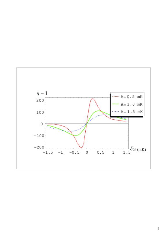
Figure 3: (Color online) The dependence of the change in cooling efficiency $\eta-1$ on the drive frequency $\delta\omega$ for different drive amplitude. $\delta\omega$ and $A$ are in milli-Kelvin units. All the other parameters are the same as those used to estimate the cooling efficiency in Sec. V.

The dependence of $\eta-1$ with respect to the drive detuning $\delta\omega$ and amplitude $A$ near degeneracy point is shown in Fig. 3. It can be seen that for a positive $\delta\omega$ (red detuning), the cooling regime is reached, and vice versa (however, note that $\eta<0$ corresponds to an unstable case rather than heating). There is no cooling or heating for zero drive $A=0$. This is consistent with optomechanical cooling. However, because of the difference between SU(2) and Heisenberg algebra, for $\delta\omega>0$, the cooling efficiency does not scale with $A$ monotonically but reaches its maximum at $A=\sqrt{2}\delta\omega$ as shown in Fig. 4. Physically, this is because too strong a drive destroys the back-action mechanism owing to its dominant rapid dynamics and even drive the qubit out of the two-level subspace. It is also shown in Fig. 3 that, as $A$ increases, the variation in the cooling efficiency with respect to $\delta\omega$ around the peak tends to become much flatter. This feature makes the cooling efficiency robust as regards operating point fluctuation by increasing the drive amplitude. However, the largest cooling efficiency also decreases with the increases in $A$. Therefore, in real experiment, a trade-off is needed to obtain both stable control and high cooling efficiency.

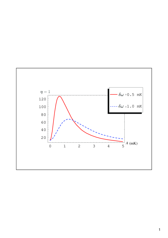
Figure 4: (Color online) The dependence of the change in the cooling efficiency $\eta-1$ on the drive amplitude $A$ with drive detuning $\delta\omega=1$ mK and $\delta\omega=5$ mK respectively. $\delta\omega$ and $A$ are in milli-Kelvin units. All the other parameters are the same as those used to estimate of cooling efficiency in Sec. V.

It is worth to mentioning that, if the qubit is biased at the degeneracy point, the second term in eq. (25) cannot be omitted. Thus we obtain a small but finite cooling effect even at the degeneracy point. Based on the first-order perturbation theory, side-band cooling is not possible at the qubit degeneracy point. However, driven Rabi oscillation at degeneracy point has been demonstrated experimentally Il’ichev et al. (2003). This is explained by fluctuation of the operating point or higher-order perturbation theory Hauss et al. (2007). It is interesting to observe that this effect is preserved by our semi-classical treatment of back-action cooling. However, based on the treatment of quantized MR, other resonant conditions may be needed if we are to study this phenomenon Hauss et al. (2007).

V Cooling efficiency in practical systems

Having obtained the effective spring constant of the Lorentz force and established the relationship between the cooling effect and the back-action mechanism, we can now estimate the cooling efficiency of this protocol for a real system. To achieve higher cooling efficiency, it is necessary to increase the mechanical quality factor $Q_{M}$ and the coupling strength $k_{L}$. A higher quality factor implies that the MR is less affected by the thermal environment. Greater coupling strength means stronger back-action damping. Moreover, as shown in Fig. 2, another crucial factor with respect to improving the cooling efficiency is the ratio between the MR frequency and the flux qubit relaxation rate, i.e., the time scales of the oscillation period and the feedback response from the qubit. Efficient cooling is achieved when the two time scales match. In self-cooling experiments with optomechanical coupling, this is one of the main experimental challenges Karrai (2006). In our proposal, the response time depends on the relaxation rate of the flux qubit. This rate can be controlled from $0.1$ MHz to $10$ MHz by controlling the initial bias magnetic flux $\Phi_{z0}$ in the $z$ direction. By controlling the high frequency ($~{}\Delta/\hbar$) noise, e.g., by deliberately attaching an external impedance to the circuit, we can change the qubit spontaneous emission time. Hence the relaxation rate of the flux qubit can be further monitored to match the frequency of the mechanical mode. This feature enables us to optimize the cooling of MR with different mode frequencies and greatly improves the cooling power.

We made our estimation based on a flux qubit loop with an aluminum Josephson junction. In this case, the relaxation time around the degeneracy point of the qubit is of the order of one hundred nanoseconds to several microseconds Yoshihara et al. (2006); Kakuyanagi et al. (2007). Hence it is suitable for a cooling MR mode with MHz frequency. For example, at an environmental temperature of $300$ mK, a flux qubit with $I_{p}=600$ nA, $\Delta=5$ GHz, $\varepsilon_{0}=1$ GHz and the relaxation rate close to the degeneracy point is $\gamma=5$ MHz. The qubit is driven by a microwave with $\omega_{d}=5.089$ GHz and $A=14.1$ MHz. When the driven qubit is used to cool a doubly-clamped Si beams Roukes (2000) with $\omega_{b}=5$ MHz, $k=0.1$ N/m, $L_{0}=5$ $\mu$m and quality factor $Q_{M}=10^{4}$, assuming $B_{0}=5$ mT, we obtain $k_{L}=2.72\times 10^{-3}$ N/m. The cooling efficiency $\eta$ is about $1.27\times 10^{2}$, which means the effective mode temperature of the MR can be cooled to about $2.36$ mK. Since $k_{L}$ is proportional to the square of the coupling magnetic field, increasing $B_{0}$ can greatly enhance the cooling power. In principle, the upper limit of $B_{0}$ is the critical magnetic field $B_{c}$ of the superconducting material in order to preserve superconductivity. For aluminum, $B_{c}\approx 9.9$ mT. But the in-plane magnetic field can be much stronger than this critical value (e.g. even larger than $100$ mT Ferguson et al. (2006)) without destroying the superconductivity. In addition, suitable arrangement of the magnetic field can result in the strong magnetic effect acting only in the MR region while being largely canceled out at the junction location. This means this cooling protocol could be potentially more powerful than the above estimation.

However, one major problem with too strong an in-plane magnetic field in the experiment is the possible tiny vibration of the sample with respect to the coupling magnetic field. With a strong magnetic field, a significant shift may be induced in the operating point by the tiny vibration. One way to solve this problem is to design the gradiometer-type flux qubit or to use an on-chip magnetic field generating coil Xue et al. (2007b).

VI Discussions

The basic idea behind our cooling protocol is similar to the self-cooling of a micro-mirror by optomechanical coupling Karrai (2006): The flux qubit plays the role of the optical cavity and the microwave drive on the qubit acts as the laser drive on the cavity. The Lorentz force produces a passive back-action on the resonator in the same way as photothermal force or radiation pressure.

However, the mathematical treatment of a two-level artificial atom is rather different from that of a bosonic field. Moreover, in practice the two systems have distinct physical nature: (1) An on-chip solid-state system without any optical component might have certain advantages as regards its application; (2) The coupling between a flux qubit and a resonator can be controlled by controlling the applied magnetic field $B_{0}$ which is independent of the qubit free Hamiltonian and microwave drive. This is different from the coupling system of a Cooper pair box and NAMR Irish and Schwab (2003) where the bias voltage $V_{g}$ modifies the coupling coefficient as well as the free Hamiltonian of the charge qubit. This feature gives the system more flexibility in terms of increasing the cooling power and switching the cooling process on and off ; (3) In order to near-resonant to laser, the frequency of the FP cavity is more than $1$ THz. To achieve efficient optomechanical cooling for a MHz oscillator, the optical quality factor of the FP cavity should be about $10^{8}$. This calls for a mirror with extremely high finesse. But in our case, it is easier to match the two energy scales since the relaxation rate at the degenerate point is typically of the order of microsecond. (4) The relaxation rate of a flux qubit, which determines the back-action response time, can be modified in situ by the bias magnetic flux in the $z$ direction. In principle with a GHz oscillator, we can work in both the $\gamma\approx\omega_{b}$ and $\gamma\ll\omega_{b}$ regimes for this Lorentz-force cooling. The latter regime is desirable for cooling towards the quantum limit Marquardt et al. (2007). This implies that our present proposal might be able to cool the MR into its quantum ground state. However, this question requires further discussion involving a consideration of quantum fluctuation.

In the above discussion, we only considered the damping of the resonator caused by the qubit via the Lorentz force. However, according to the fluctuation-dissipation theorem, fluctuation is always associated with dissipation. Additional fluctuation is also induced by the back-action of the qubit system. For a more comprehensive description, we need to take this fluctuation into account. The additional fluctuation can be represented by an effective temperature $T_{1}$. Therefore, the resonator is effectively in contact with two different baths Martin et al. (2004); Clerk and Bennett (2005); Blencowe et al. (2005), one is the real environment with temperature $T_{0}$, and damping rate $\Gamma$ and the other is the effective bath with effective temperature $T_{1}$, and damping rate $\Gamma_{1}$. Physically, the effective bath is formed by the lossy qubit under microwave drive. The temperature of the MR reaches a balance between the two baths as

$$T_{\text{eff}}=\frac{\Gamma T_{0}+\Gamma_{1}T_{1}}{\Gamma+\Gamma_{1}}\ .$$ (29)

The near-resonant microwave drive largely suppresses the fluctuation (see Appendix)

$$\exp\left(\frac{\omega_{b}}{T_{1}}\right)\sim\left(\frac{1-\cos\beta_{0}}{1+\cos\beta_{0}}\right)^{2}\sim 1.$$ (30)

Therefore we obtain $T_{1}\sim\omega_{b}\ll T_{0}\sim\Omega$, which means the fluctuation caused by the qubit can be effectively disregarded, as far as the spontaneous emission of the qubit is concerned. A more realistic estimation of this fluctuation requires detailed information about the quantum noise of the qubit.

The cooling of the MR could be measured by using the conventional motion transduction method Schwab and Roukes (2005). In this system, it can also be revealed by the reduction in the integration of the power spectrum for the MR $\left\langle z^{2}\left(\omega\right)\right\rangle$. Since

$$\delta I=\frac{2\sqrt{2}A\delta\omega}{A^{2}+2\delta\omega^{2}}\frac{B_{0}I_{p}L_{0}}{\Delta}\delta z,$$ (31)

the motion power spectrum is proportional to the current power spectrum. The MR power spectrum can be recorded by detecting the current in the loop. The current in the flux qubit loop can be recorded with a dc SQUID switching measurement or with a more sophisticated phase sensitive dispersive readout such as Josephson bifurcation measurement Siddiqi et al. (2004).

Appendix: The dissipative dynamics of the qubit

The dissipative dynamics of the qubit is governed by the following master equation

$$\dot{\rho}=-\frac{i}{\hbar}\left[H_{q},\rho\right]+\mathcal{L}\rho$$ (32)

where $\rho$ is the reduced density matrix of the qubit, $H_{q}$ is the qubit Hamiltonian in eq. (10) and $\mathcal{L}$ is the Liouvillian characterizing the influence of the environment.

As regards the qubit, we only consider the spontaneous emission with rate $\Gamma_{0}$ and neglect the excitation and dephasing terms because the qubit energy spacing is much larger than the environment temperature and the qubit is biased close to the degeneracy point

$$\mathcal{L}\rho=\frac{\Gamma_{0}}{2}\left(2\sigma_{-}\rho\sigma_{+}-\rho\sigma_{+}\sigma_{-}-\sigma_{+}\sigma_{-}\rho\right).$$ (33)

By successively applying three unitary transformations to eq. (32) Li (2007) or making use of the Fermi golden rule Hauss et al. (2007), we can readily obtain the master equation in the interaction picture of the rotating frame

$$\dot{\rho}_{I}^{R}=\mathcal{L}^{R}\rho_{I}^{R},$$ (34)

where

$$\mathcal{L}^{R}\rho_{I}^{R} = \frac{\Gamma_{\downarrow}}{2}\left(2\tilde{\sigma}_{-}\rho_{I}^{R}\tilde{\sigma}_{+}-\rho_{I}^{R}\tilde{\sigma}_{+}\tilde{\sigma}_{-}-\tilde{\sigma}_{+}\tilde{\sigma}_{-}\rho_{I}^{R}\right)$$ (35)

$$+\frac{\Gamma_{\uparrow}}{2}\left(2\tilde{\sigma}_{+}\rho_{I}^{R}\tilde{\sigma}_{-}-\rho_{I}^{R}\tilde{\sigma}_{-}\tilde{\sigma}_{+}-\tilde{\sigma}_{-}\tilde{\sigma}_{+}\rho_{I}^{R}\right)$$

$$+\frac{\Gamma_{\varphi}}{2}\left(\tilde{\sigma}_{z}\rho_{I}^{R}\tilde{\sigma}_{z}-\rho_{I}^{R}\right),$$

with

$$\Gamma_{\downarrow} = \frac{\Gamma_{0}}{4}\left(1+\cos\beta\right)^{2},$$

$$\Gamma_{\uparrow} = \frac{\Gamma_{0}}{4}\left(1-\cos\beta\right)^{2},$$

$$\Gamma_{\varphi} = \frac{\Gamma_{0}}{2}\sin^{2}\beta$$ (36)

and $\Gamma_{0}$ is the spontaneous emission rate. This master equation shows that the effective bath formed by the driven qubit in dissipative environment is

$$\exp\left(\frac{\omega_{b}}{T_{1}}\right)\equiv\frac{\Gamma_{\downarrow}}{\Gamma_{\uparrow}}=\left(\frac{1+\cos\beta_{0}}{1-\cos\beta_{0}}\right)^{2}$$ (37)

Therefore, in the interaction picture the equations of motion for the average value of the qubit operators are

$$\frac{d}{dt}\left\langle\tilde{\sigma}_{+}\left(t\right)\right\rangle = -\frac{\left(\Gamma_{\uparrow}+\Gamma_{\downarrow}+2\Gamma_{\varphi}\right)}{2}\left\langle\tilde{\sigma}_{+}\left(t\right)\right\rangle,$$

$$\frac{d}{dt}\left\langle\tilde{\sigma}_{-}\left(t\right)\right\rangle = -\frac{\left(\Gamma_{\uparrow}+\Gamma_{\downarrow}+2\Gamma_{\varphi}\right)}{2}\left\langle\tilde{\sigma}_{-}\left(t\right)\right\rangle,$$

$$\frac{d}{dt}\left\langle\tilde{\sigma}_{z}\left(t\right)\right\rangle = -\left(\Gamma_{\uparrow}+\Gamma_{\downarrow}\right)\left\langle\tilde{\sigma}_{z}\left(t\right)\right\rangle-\left(\Gamma_{\uparrow}-\Gamma_{\downarrow}\right).$$ (38)

Setting $d\langle\sigma_{i}\rangle/dt=0$, we can obtain the steady-state solution of the qubit in a dissipative system

$$\left\langle\tilde{\sigma}_{+}\right\rangle_{s} = \left\langle\tilde{\sigma}_{-}\right\rangle_{s}=0,$$

$$\left\langle\tilde{\sigma}_{z}\right\rangle_{s} = -\frac{\Gamma_{\uparrow}-\Gamma_{\downarrow}}{\Gamma_{\uparrow}+\Gamma_{\downarrow}}=-\frac{2\cos\beta\left(z\right)}{1+\cos^{2}\beta\left(z\right)}.$$ (39)

Making use of eq. (39) and the transformation relations eqs. (12), (16) and (18), it turns out that the quantity of interest in the experimental frame is related to those in the rotating frame as

$$\left\langle\sigma_{z}\right\rangle_{s}=\left(\cos\theta\left(z\right)\cos\beta\left(z\right)-\sin\theta\left(z\right)\sin\beta\left(z\right)\cos\omega_{d}t\right)\left\langle\tilde{\sigma}_{z}\right\rangle_{s}.$$ (40)

Neglecting the high-frequency oscillating term, we obtain the effective value in eq. (21)

$$\left\langle\sigma_{z}\right\rangle_{s}=-\frac{2\cos^{2}\beta\left(z\right)}{1+\cos^{2}\beta\left(z\right)}\cos\theta\left(z\right)$$ (41)

References

- Cleland (2002) A. N. Cleland, Foundations of Nanomechanics: From Solid-state Theory to Device Applications (Springer-Verlag, Berlin, 2002).
- Blencowe (2004) M. Blencowe, Phys. Rep. 395, 159 (2004).
- LaHaye et al. (2004) M. D. LaHaye, O. Buu, B. Camarota, and K. C. Schwab, Science 304, 74 (2004).
- Cohadon et al. (1999) P. F. Cohadon, A. Heidmann, and M. Pinard, Phys. Rev. Lett. 83, 3174 (1999).
- Kleckner and Bouwmeester (2006) D. Kleckner and D. Bouwmeester, Nature (London) 444, 75 (2006).
- Poggio et al. (2007) M. Poggio, C. L. Degen, H. J. Mamin, and D. Rugar, Phys. Rev. Lett. 99, 017201 (2007).
- Metzger and Karrai (2004) C. H. Metzger and K. Karrai, Nature (London) 432, 1002 (2004).
- Gigan et al. (2006) S. Gigan, H. R. Bohm, M. Paternostro, F. Blaser, G. Langer, J. B. Hertzberg, K. C. Schwab, D. Bauerle, M. Aspelmeyer, and A. Zeilinger, Nature (London) 444, 67 (2006).
- Arcizet et al. (2006) O. Arcizet, R. F. Cohadon, T. Briant, M. Pinard, and A. Heidmann, Nature (London) 444, 71 (2006).
- Schliesser et al. (2006) A. Schliesser, P. Del Haye, N. Nooshi, K. J. Vahala, and T. J. Kippenberg, Phys. Rev. Lett. 97, 243905 (2006).
- Naik et al. (2006) A. Naik, O. Buu, M. D. LaHaye, A. D. Armour, A. A. Clerk, M. P. Blencowe, and K. C. Schwab, Nature (London) 443, 193 (2006).
- Hopkin et al. (2003) A. Hopkin, K. Jacobs, S. Habib, and K. Schwab, Phys. Rev. B 68, 235328 (2003).
- Wilson-Rae et al. (2004) I. Wilson-Rae, P. Zoller, and A. Imamoglu, Phys. Rev. Lett. 92, 075507 (2004).
- Martin et al. (2004) I. Martin, A. Shnirman, L. Tian, and P. Zoller, Phys. Rev. B 69, 125339 (2004).
- Zhang et al. (2005) P. Zhang, Y. D. Wang, and C. P. Sun, Phys. Rev. Lett. 95, 097204 (2005).
- Brown et al. (2007) K. R. Brown, J. Britton, R. J. Epstein, J. Chiaverini, D. Leibfried, and D. J. Wineland, Phys. Rev. Lett. 99, 137205 (2007).
- Xue et al. (2007a) F. Xue, Y. D. Wang, Y.-x. Liu, and F. Nori, Phys. Rev. B 76, 205302 (2007a).
- Corbitt et al. (2007) T. Corbitt, Y. Chen, E. Innerhofer, H. Mu ller-Ebhardt, D. Ottaway, H. Rehbein, D. Sigg, S. Whitcomb, C. Wipf, and N. Mavalvala, Phys. Rev. Lett. 98, 150802 (2007).
- Thompson et al. (2007) J. D. Thompson, B. M. Zwickl, A. M. Jayich, F. Marquardt, S. M. Girvin, and J. G. E. Harris, ArXiv:0707.1724 (2007).
- Mow-Lowry et al. (2008) C. M. Mow-Lowry, A. J. Mullavey, S. Go ler, M. B. Gray, and D. E. McClelland, Phys. Rev. Lett. 100, 010801 (2008).
- You et al. (2008) J. Q. You, Yu-xi Liu, and Franco Nori, Phys. Rev. Lett. 100, 047001 (2008).
- Marquardt et al. (2007) F. Marquardt, J. P. Chen, A. A. Clerk, and S. M. Girvin, Phys. Rev. Lett. 99, 093902 (2007).
- Genes et al. (2007) C. Genes, D. Vitali, P. Tombesi, S. Gigan, and M. Aspelmeyer, arXiv:0705.1728 (2007).
- Wilson-Rae et al. (2007) I. Wilson-Rae, N. Nooshi, W. Zwerger, and T. Kippenberg, Phys. Rev. Lett. 99, 093901 (2007).
- Braginsky and Vyatchanin (2002) V. B. Braginsky and S. P. Vyatchanin, Phys. Lett. A 293, 228 (2002).
- Mooij et al. (1999) J. E. Mooij, T. P. Orlando, L. Levitov, L. Tian, C. H. van der Wal, and S. Lloyd, Science 285, 1036 (1999).
- Orlando et al. (1999) T. P. Orlando, J. E. Mooij, L. Tian, C. H. van der Wal, L. S. Levitov, S. Lloyd, and J. J. Mazo, Phys. Rev. B 60, 15398 (1999).
- Wilhelm and Semba (2006) F. K. Wilhelm and K. Semba, in Physical Realization of Quantum Computing (World Scientific, Singapore, 2006).
- Xue et al. (2007b) F. Xue, Y. D. Wang, C. P. Sun, H. Okamoto, H. Yamaguchi, and K. Semba, New J. Phys. 9, 35 (2007b).
- Gaidarzhy et al. (2005) A. Gaidarzhy, G. Zolfagharkhani, R. L. Badzey, and P. Mohanty, Phys. Rev. Lett. 94, 030402 (2005).
- Clerk and Bennett (2005) A. A. Clerk and S. Bennett, New J. Phys. 7, 238 (2005).
- Blencowe et al. (2005) M. P. Blencowe, J. Imbers, and A. D. Armour, New J. Phys. 7, 236 (2005).
- Poncharal et al. (1999) P. Poncharal, Z. L. Wang, D. Ugarte, and W. A. d. Heer, Science 283, 1513 (1999).
- Chiorescu et al. (2003) I. Chiorescu, Y. Nakamura, C. J. P. M. Harmans, and J. E. Mooij, Science 299, 1869 (2003).
- Saito et al. (2004) S. Saito, M. Thorwart, H. Tanaka, M. Ueda, H. Nakano, K. Semba, and H. Takayanagi, Phys. Rev. Lett. 93, 037001 (2004).
- Valenzuela et al. (2006) S. O. Valenzuela, W. D. Oliver, D. M. Berns, K. K. Berggren, L. S. Levitov, and T. P. Orlando, Science 314, 1589 (2006).
- Zhou and Mizel (2006) X. Zhou and A. Mizel, Phys. Rev. Lett. 97, 267201 (2006).
- Buks and Blencowe (2006) E. Buks and M. P. Blencowe, Phys. Rev. B 74, 174504 (2006).
- Blencowe and Buks (2007) M. P. Blencowe and E. Buks, Phys. Rev. B 76, 014511 (2007).
- Yoshihara et al. (2006) F. Yoshihara, K. Harrabi, A. O. Niskanen, Y. Nakamura, and J. S. Tsai, Phys. Rev. Lett. 97, 167001 (2006).
- Kakuyanagi et al. (2007) K. Kakuyanagi, T. Meno, S. Saito, H. Nakano, K. Semba, H. Takayanagi, F. Deppe, and A. Shnirman, Phys. Rev. Lett. 98, 047004 (2007).
- Il’ichev et al. (2003) E. Il’ichev and et al., Phys. Rev. Lett. 91, 097906 (2003).
- Hauss et al. (2007) J. Hauss, A. Fedorov, C. Hutter, A. Shnirman, and G. Schoen, cond-mat/00701041 (2007).
- Karrai (2006) K. Karrai, Nature (London) 444, 41 (2006).
- Roukes (2000) M. L. Roukes, in 2000 Solid-state Sensor and Actuator Workshop (2000).
- Ferguson et al. (2006) A. J. Ferguson, S. E. Andresen, R. Brenner, and R. G. Clark, Phys. Rev. Lett. 97, 086602 (2006).
- Irish and Schwab (2003) E. K. Irish and K. Schwab, Phys. Rev. B 68, 155311 (2003).
- Schwab and Roukes (2005) K. C. Schwab and M. L. Roukes, Physics Today 58, 36 (2005).
- Siddiqi et al. (2004) I. Siddiqi, R. Vijay, F. Pierre, C. M.Wilson, M. Metcalfe, C. Rigetti, L. Frunzio, and M. H. Devoret, Phys. Rev. Lett. 93, 207002 (2004).
- Li (2007) Y. Li, private communication (2007).