AMBRE – a Mathematica package for the construction of Mellin-Barnes representations for Feynman integrals

J. Gluza, K. Kajda Department of Field Theory and Particle Physics, Institute of Physics,
University of Silesia, Uniwersytecka 4, PL-40-007 Katowice, Poland
T. Riemann Deutsches Elektronen-Synchrotron, DESY,
Platanenallee 6, 15738 Zeuthen, Germany
Abstract

The Mathematica toolkit AMBRE derives Mellin-Barnes (MB) representations for Feynman integrals in d=42ε𝑑42𝜀d=4-2\varepsilon dimensions. It may be applied for tadpoles as well as for multi-leg multi-loop scalar and tensor integrals. AMBRE uses a loop-by-loop approach and aims at lowest dimensions of the final MB representations. The present version of AMBRE works fine for planar Feynman diagrams. The output may be further processed by the package MB for the determination of its singularity structure in ε𝜀\varepsilon. The AMBRE package contains various sample applications for Feynman integrals with up to six external particles and up to four loops.

DESY 07-037

HEPTOOLS 07-009

SFB/CPP-07-14

1 Introduction

Recently, Mellin-Barnes (MB) representations of Feynman integrals have been used extensively in various phenomenological and theoretical studies of quantum field theory. In many applications, sometimes in quite sophisticated ones [1, 2, 3], the MB-integrals can be solved analytically. One also may merge knowledge of some analytical solutions given by MB-integrals with other methods, e.g. the differential equations approach, as demonstrated in [4]. An introduction to the subject with many examples may be found in the monographies [5, 6]. A systematic derivation and numerical evaluation of MB-representations for Feynman integrals with a (unpublished) Maple package was described in [7]. At the same time, the Mathematica program MB for the automatized analytic continuation of MB-integrals was published in [8]. With AMBRE, we deliver a Mathematica tool for the derivation of MB-integrals and their subsequent analytic continuation and numerical evaluation with MB.

The article is organized as follows. In section 2 we introduce the formulae used for the MB-representation of a general Feynman integral. The basic features of AMBRE are described in section 3. One-loop examples are given in section 4. Section 5 describes the implementation of the loop-by-loop approach to multi-loop integrals. Examples with tadpoles and on-shell diagrams as well as problems related to non-planar topologies are discussed in sections 68. A summary follows in section 9. In an appendix we list the Mathematica functions of AMBRE.

2 Construction of Mellin-Barnes representations

The backbone of the procedure to build up MB-representations with AMBRE is the relation

1(A+B)ν=Bν2πiΓ(ν)ii𝑑σAσBσΓ(σ)Γ(ν+σ),1superscript𝐴𝐵𝜈superscript𝐵𝜈2𝜋𝑖Γ𝜈superscriptsubscript𝑖𝑖differential-d𝜎superscript𝐴𝜎superscript𝐵𝜎Γ𝜎Γ𝜈𝜎\displaystyle\frac{1}{(A+B)^{\nu}}=\frac{B^{-\nu}}{2\pi i\Gamma{(\nu)}}\int\limits_{-i\infty}^{i\infty}d\sigma{A^{\sigma}~{}B^{-\sigma}}~{}\Gamma{(-\sigma)}\Gamma{(\nu+\sigma)}, (1)

where the integration contour separates the poles of the ΓΓ\Gamma-functions.

The object to be evaluated by AMBRE is an L𝐿L-loop Feynman integral111Often one uses the additional normalization eεγELsuperscript𝑒𝜀subscript𝛾𝐸𝐿e^{\varepsilon\gamma_{E}L}; we leave this to the later evaluation with the package MB [8]. in d=42ε𝑑42𝜀d=4-2\varepsilon dimensions with N𝑁N internal lines with momenta qisubscript𝑞𝑖q_{i} and masses misubscript𝑚𝑖m_{i}, and E𝐸E external legs with momenta pesubscript𝑝𝑒p_{e}:

GL[T(k)]=1(iπd/2)Lddk1ddkLT(k)(q12m12)ν1(qi2mi2)νj(qN2mN2)νN.subscript𝐺𝐿delimited-[]𝑇𝑘1superscript𝑖superscript𝜋𝑑2𝐿superscript𝑑𝑑subscript𝑘1superscript𝑑𝑑subscript𝑘𝐿𝑇𝑘superscriptsuperscriptsubscript𝑞12superscriptsubscript𝑚12subscript𝜈1superscriptsuperscriptsubscript𝑞𝑖2superscriptsubscript𝑚𝑖2subscript𝜈𝑗superscriptsuperscriptsubscript𝑞𝑁2superscriptsubscript𝑚𝑁2subscript𝜈𝑁\displaystyle G_{L}[T(k)]=\frac{1}{(i\pi^{d/2})^{L}}\int\frac{d^{d}k_{1}\ldots d^{d}k_{L}~{}~{}T(k)}{(q_{1}^{2}-m_{1}^{2})^{\nu_{1}}\ldots(q_{i}^{2}-m_{i}^{2})^{\nu_{j}}\ldots(q_{N}^{2}-m_{N}^{2})^{\nu_{N}}}. (2)

The numerator T(k)𝑇𝑘T(k) is a tensor in the integration variables:

T(k)𝑇𝑘\displaystyle T(k) =\displaystyle= 1,klμ,klμknν,1superscriptsubscript𝑘𝑙𝜇superscriptsubscript𝑘𝑙𝜇superscriptsubscript𝑘𝑛𝜈\displaystyle 1,k_{l}^{\mu},k_{l}^{\mu}k_{n}^{\nu},\ldots (3)

The momenta of the denominator functions disubscript𝑑𝑖d_{i} may be expressed by external and loop momenta:

disubscript𝑑𝑖\displaystyle d_{i} =\displaystyle= qi2mi2=(l=1LαilklPi)2mi2=(l=1Lαilkle=1Eβiepe)2mi2.superscriptsubscript𝑞𝑖2superscriptsubscript𝑚𝑖2superscriptsuperscriptsubscript𝑙1𝐿subscript𝛼𝑖𝑙subscript𝑘𝑙subscript𝑃𝑖2superscriptsubscript𝑚𝑖2superscriptsuperscriptsubscript𝑙1𝐿subscript𝛼𝑖𝑙subscript𝑘𝑙superscriptsubscript𝑒1𝐸subscript𝛽𝑖𝑒subscript𝑝𝑒2superscriptsubscript𝑚𝑖2\displaystyle q_{i}^{2}-m_{i}^{2}~{}=~{}\left(\sum_{l=1}^{L}\alpha_{il}k_{l}-P_{i}\right)^{2}-m_{i}^{2}~{}=~{}\left(\sum_{l=1}^{L}\alpha_{il}k_{l}-\sum_{e=1}^{E}\beta_{ie}p_{e}\right)^{2}-m_{i}^{2}. (4)

In the package AMBRE, in a first step the momentum integrals are replaced by Feynman parameter integrals:

GL[T(k)]subscript𝐺𝐿delimited-[]𝑇𝑘\displaystyle G_{L}[T(k)] =\displaystyle= (1)NνΓ(Nνd2L)i=1NΓ(νi)01j=1Ndxjxjνj1δ(1i=1Nxi)U(x)Nνd(L+1)/2F(x)NνdL/2PL(T)superscript1subscript𝑁𝜈Γsubscript𝑁𝜈𝑑2𝐿superscriptsubscriptproduct𝑖1𝑁Γsubscript𝜈𝑖superscriptsubscript01superscriptsubscriptproduct𝑗1𝑁𝑑subscript𝑥𝑗superscriptsubscript𝑥𝑗subscript𝜈𝑗1𝛿1superscriptsubscript𝑖1𝑁subscript𝑥𝑖𝑈superscript𝑥subscript𝑁𝜈𝑑𝐿12𝐹superscript𝑥subscript𝑁𝜈𝑑𝐿2subscript𝑃𝐿𝑇\displaystyle\frac{(-1)^{N_{\nu}}\Gamma\left(N_{\nu}-\frac{d}{2}L\right)}{\prod_{i=1}^{N}\Gamma(\nu_{i})}\int_{0}^{1}\prod_{j=1}^{N}dx_{j}~{}x_{j}^{\nu_{j}-1}\delta(1-\sum_{i=1}^{N}x_{i})\frac{U(x)^{N_{\nu}-d(L+1)/2}}{F(x)^{N_{\nu}-dL/2}}~{}P_{L}(T)

with

Nνsubscript𝑁𝜈\displaystyle N_{\nu} =\displaystyle= i=1Nνi.superscriptsubscript𝑖1𝑁subscript𝜈𝑖\displaystyle\sum_{i=1}^{N}\nu_{i}. (6)

The two functions U𝑈U and F𝐹F are characteristics of the topology of the Feynman integral. One may derive them from

𝒩𝒩\displaystyle{\mathcal{N}} =\displaystyle= i=1Nxi(qi2mi2)kMk2kQ+J,superscriptsubscript𝑖1𝑁subscript𝑥𝑖superscriptsubscript𝑞𝑖2superscriptsubscript𝑚𝑖2𝑘𝑀𝑘2𝑘𝑄𝐽\displaystyle\sum_{i=1}^{N}x_{i}(q_{i}^{2}-m_{i}^{2})~{}\equiv~{}kMk-2kQ+J, (7)

where Mll=i=1Nαilαilxisubscript𝑀𝑙superscript𝑙superscriptsubscript𝑖1𝑁subscript𝛼𝑖superscript𝑙subscript𝛼𝑖𝑙subscript𝑥𝑖M_{ll^{\prime}}=\sum_{i=1}^{N}\alpha_{il^{\prime}}\alpha_{il}x_{i}, and Ql=i=1NαilPixisubscript𝑄𝑙superscriptsubscript𝑖1𝑁subscript𝛼𝑖𝑙subscript𝑃𝑖subscript𝑥𝑖Q_{l}=\sum_{i=1}^{N}\alpha_{il}P_{i}x_{i}, and J=i=1N(Pi2mi2)xi𝐽superscriptsubscript𝑖1𝑁superscriptsubscript𝑃𝑖2superscriptsubscript𝑚𝑖2subscript𝑥𝑖J=\sum_{i=1}^{N}(P_{i}^{2}-m_{i}^{2})x_{i}; namely:

U(x)𝑈𝑥\displaystyle U{(x)} =\displaystyle= det(M),det𝑀\displaystyle\textrm{det}(M), (8)
F(x)𝐹𝑥\displaystyle F({x}) =\displaystyle= det(M)J+QM~Q.det𝑀𝐽𝑄~𝑀𝑄\displaystyle-\textrm{det}(M)~{}J+Q\tilde{M}Q. (9)

The U𝑈U and F𝐹F as well as M~=det(M)M1~𝑀det𝑀superscript𝑀1\tilde{M}=\textrm{det}(M)~{}M^{-1} are polynomials in x𝑥x, and so are the numerator functions PL(T)subscript𝑃𝐿𝑇P_{L}(T) in (2) for scalar and vector integrals:

PL(1)subscript𝑃𝐿1\displaystyle P_{L}(1) =\displaystyle= 1,1\displaystyle 1, (10)
PL(klα)subscript𝑃𝐿superscriptsubscript𝑘𝑙𝛼\displaystyle P_{L}(k_{l}^{\alpha}) =\displaystyle= l=1LM~llQlα.superscriptsubscriptsuperscript𝑙1𝐿subscript~𝑀𝑙superscript𝑙superscriptsubscript𝑄superscript𝑙𝛼\displaystyle\sum_{l^{\prime}=1}^{L}{\tilde{M}}_{ll^{\prime}}Q_{l^{\prime}}^{\alpha}. (11)

Tensors of higher degree depend additionally on the diagonalizing rotation V𝑉V for 𝒩𝒩\mathcal{N},

𝒩diag=(α1,,αL)=(V1)+MV1,subscript𝒩𝑑𝑖𝑎𝑔subscript𝛼1subscript𝛼𝐿superscriptsuperscript𝑉1𝑀superscript𝑉1\displaystyle{\mathcal{N}}_{diag}=(\alpha_{1},\ldots,\alpha_{L})~{}=~{}(V^{-1})^{+}MV^{-1}, (12)

and become non-polynomial in x𝑥x. As an example, we quote here the case of an L𝐿L-loop integral with a tensor of degree two:

PL(klαklβ)subscript𝑃𝐿superscriptsubscript𝑘𝑙𝛼superscriptsubscript𝑘superscript𝑙𝛽\displaystyle P_{L}(k_{l}^{\alpha}k_{l^{\prime}}^{\beta}) =\displaystyle= i=1L[[M~liQi]α[M~liQi]βΓ(Nνd2L1)Γ(Nνd2L)UF(Vli1)+(Vli1)αigαβ2].superscriptsubscript𝑖1𝐿delimited-[]superscriptdelimited-[]subscript~𝑀𝑙𝑖subscript𝑄𝑖𝛼superscriptdelimited-[]subscript~𝑀superscript𝑙𝑖subscript𝑄𝑖𝛽Γsubscript𝑁𝜈𝑑2𝐿1Γsubscript𝑁𝜈𝑑2𝐿𝑈𝐹superscriptsuperscriptsubscript𝑉𝑙𝑖1superscriptsubscript𝑉superscript𝑙𝑖1subscript𝛼𝑖superscript𝑔𝛼𝛽2\displaystyle\sum_{i=1}^{L}\Biggl{[}[{\tilde{M}}_{li}Q_{i}]^{\alpha}[{\tilde{M}}_{l^{\prime}i}Q_{i}]^{\beta}-\frac{\Gamma\left(N_{\nu}-\frac{d}{2}L-1\right)}{\Gamma\left(N_{\nu}-\frac{d}{2}L\right)}UF\frac{(V_{li}^{-1})^{+}(V_{l^{\prime}i}^{-1})}{\alpha_{i}}~{}\frac{g^{\alpha\beta}}{2}\Biggr{]}. (13)

The formulae simplify considerably for one-loop integrals:

U𝑈\displaystyle U =\displaystyle= M=M~=det(M)=V=iNxi=1,𝑀~𝑀det𝑀𝑉superscriptsubscript𝑖𝑁subscript𝑥𝑖1\displaystyle M~{}=~{}{\tilde{M}}~{}=~{}\textrm{det}(M)~{}=~{}V~{}=~{}\sum_{i}^{N}x_{i}~{}=~{}1, (14)
F𝐹\displaystyle F =\displaystyle= UJ+Q2=i,jN[PiPjPi2+mi2]xixjijNfijxixj.𝑈𝐽superscript𝑄2superscriptsubscript𝑖𝑗𝑁delimited-[]subscript𝑃𝑖subscript𝑃𝑗superscriptsubscript𝑃𝑖2superscriptsubscript𝑚𝑖2subscript𝑥𝑖subscript𝑥𝑗superscriptsubscript𝑖𝑗𝑁subscript𝑓𝑖𝑗subscript𝑥𝑖subscript𝑥𝑗\displaystyle-UJ+Q^{2}~{}=~{}\sum_{i,j}^{N}[P_{i}P_{j}-P_{i}^{2}+m_{i}^{2}]x_{i}x_{j}~{}\equiv~{}\sum_{i\leq j}^{N}f_{ij}x_{i}x_{j}. (15)

Then, the tensor factors P1(T)subscript𝑃1𝑇P_{1}(T) in (2) will become:

P1(1)subscript𝑃11\displaystyle P_{1}(1) =\displaystyle= 1,1\displaystyle 1, (16)
P1(kα)subscript𝑃1superscript𝑘𝛼\displaystyle P_{1}(k^{\alpha}) =\displaystyle= i=1NxiPiα,superscriptsubscript𝑖1𝑁subscript𝑥𝑖superscriptsubscript𝑃𝑖𝛼\displaystyle\sum_{i=1}^{N}x_{i}P_{i}^{\alpha}, (17)
P1(kαkβ)subscript𝑃1superscript𝑘𝛼superscript𝑘𝛽\displaystyle P_{1}(k^{\alpha}k^{\beta}) =\displaystyle= i=1NxiPiαj=1NxjPjβΓ(Nνd21)Γ(Nνd2)Fgαβ2, etc.,superscriptsubscript𝑖1𝑁subscript𝑥𝑖superscriptsubscript𝑃𝑖𝛼superscriptsubscript𝑗1𝑁subscript𝑥𝑗superscriptsubscript𝑃𝑗𝛽Γsubscript𝑁𝜈𝑑21Γsubscript𝑁𝜈𝑑2𝐹superscript𝑔𝛼𝛽2 etc.,\displaystyle\sum_{i=1}^{N}x_{i}P_{i}^{\alpha}\sum_{j=1}^{N}x_{j}P_{j}^{\beta}-\frac{\Gamma\left(N_{\nu}-\frac{d}{2}-1\right)}{\Gamma\left(N_{\nu}-\frac{d}{2}\right)}~{}F~{}\frac{g^{\alpha\beta}}{2},\textrm{~{}~{}etc.,} (18)

with Piαsuperscriptsubscript𝑃𝑖𝛼P_{i}^{\alpha} being the so-called chords introduced in (4). For the general case P1(T)subscript𝑃1𝑇P_{1}(T) see section 4.2.

One now has to perform the x𝑥x-integrations. In AMBRE, we will do this by the following simple formula:

01i=1Ndxixiqi1δ(1jxj)superscriptsubscript01superscriptsubscriptproduct𝑖1𝑁𝑑subscript𝑥𝑖superscriptsubscript𝑥𝑖subscript𝑞𝑖1𝛿1subscript𝑗subscript𝑥𝑗\displaystyle\int_{0}^{1}\prod_{i=1}^{N}dx_{i}~{}x_{i}^{q_{i}-1}~{}\delta\left(1-\sum_{j}x_{j}\right) =\displaystyle= Γ(q1)Γ(qN)Γ(q1++qN).Γsubscript𝑞1Γsubscript𝑞𝑁Γsubscript𝑞1subscript𝑞𝑁\displaystyle\frac{\Gamma(q_{1})\cdots\Gamma(q_{N})}{\Gamma\left(q_{1}+\cdots+q_{N}\right)}. (19)

From the above text it is evident that the integrand of (2) contains besides simple sums of monomials ixinisubscriptproduct𝑖superscriptsubscript𝑥𝑖subscript𝑛𝑖\prod_{i}x_{i}^{n_{i}} also different structures. This is due to the appearance of the factors U(x)𝑈𝑥U(x) and F(x)𝐹𝑥F(x). Beginning with two-loop tensor integrals, one faces additionally a complicated dependence of P(T)𝑃𝑇P(T) on x𝑥x for higher rank tensors T𝑇T due to the appearence of V𝑉V and α𝛼\alpha, see (13).

For this reason, the present version of AMBRE is restricted to scalar and vector integrals and/or to one-loop integrals. In these cases one may rewrite F(x)𝐹𝑥F(x) and U(x)𝑈𝑥U(x) so that (19) becomes applicable; for the one-loop case only the F(x)𝐹𝑥F(x). That is why we discuss here only the F(x)𝐹𝑥F(x). From (15), the F(x)𝐹𝑥F(x) may be written as a sum of NF12N(N+1)subscript𝑁𝐹12𝑁𝑁1N_{F}\leq\frac{1}{2}N(N+1) non-vanishing, bilinear terms in xisubscript𝑥𝑖x_{i}:

F(x)(NνdL/2)𝐹superscript𝑥subscript𝑁𝜈𝑑𝐿2\displaystyle F(x)^{-(N_{\nu}-dL/2)} =\displaystyle= [n=1NFfn(i,j)xixj](NνdL/2)superscriptdelimited-[]superscriptsubscript𝑛1subscript𝑁𝐹subscript𝑓𝑛𝑖𝑗subscript𝑥𝑖subscript𝑥𝑗subscript𝑁𝜈𝑑𝐿2\displaystyle\left[\sum_{n=1}^{N_{F}}f_{n}(i,j)x_{i}x_{j}\right]^{-(N_{\nu}-dL/2)}
=\displaystyle= 1Γ(NνdL/2)1(2πi)NFi=1NFi+uii+ui𝑑zin=2NF[fn(ij)xixj]zn1Γsubscript𝑁𝜈𝑑𝐿21superscript2𝜋𝑖subscript𝑁𝐹superscriptsubscriptproduct𝑖1subscript𝑁𝐹superscriptsubscript𝑖subscript𝑢𝑖𝑖subscript𝑢𝑖differential-dsubscript𝑧𝑖superscriptsubscriptproduct𝑛2subscript𝑁𝐹superscriptdelimited-[]subscript𝑓𝑛𝑖𝑗subscript𝑥𝑖subscript𝑥𝑗subscript𝑧𝑛\displaystyle\frac{1}{\Gamma(N_{\nu}-dL/2)}\frac{1}{(2\pi i)^{N_{F}}}\prod_{i=1}^{N_{F}}\int\limits_{-i\infty+u_{i}}^{i\infty+u_{i}}dz_{i}\prod_{n=2}^{N_{F}}\left[f_{n}(ij)x_{i}x_{j}\right]^{z_{n}}
[f1(ij)xixj](NνdL/2)j=2NFzjΓ(NνdL2+j=2NFzj)j=2NFΓ(zj).superscriptdelimited-[]subscript𝑓1𝑖𝑗subscript𝑥𝑖subscript𝑥𝑗subscript𝑁𝜈𝑑𝐿2superscriptsubscript𝑗2subscript𝑁𝐹subscript𝑧𝑗Γsubscript𝑁𝜈𝑑𝐿2superscriptsubscript𝑗2subscript𝑁𝐹subscript𝑧𝑗superscriptsubscriptproduct𝑗2subscript𝑁𝐹Γsubscript𝑧𝑗\displaystyle~{}\left[f_{1}(ij)x_{i}x_{j}\right]^{-(N_{\nu}-dL/2)-\sum_{j=2}^{N_{F}}z_{j}}\Gamma\left(N_{\nu}-\frac{dL}{2}+\sum_{j=2}^{N_{F}}z_{j}\right)\prod_{j=2}^{N_{F}}\Gamma(-z_{j}).

Here, fn(i,j)=fijsubscript𝑓𝑛𝑖𝑗subscript𝑓𝑖𝑗f_{n}(i,j)=f_{ij} if fij0subscript𝑓𝑖𝑗0f_{ij}\neq 0. Inserting (2) (and if needed a similar representation for the U(x)𝑈𝑥U(x)) and the tensor function P(T)𝑃𝑇P(T) into (2) allows to apply (19) for an evaluation of the x𝑥x-integrations.

As a result, any scalar Feynman integral may be represented by a single multi-dimensional MB-integral and L𝐿L-loop tensor integrals by finite sums of MB-integrals. With AMBRE we will evaluate the L𝐿L-loop integrals by a loop-by-loop technique, which essentially allows us to restrict the formalism to the one-loop case. By the examples it will be seen that this is a powerful ansatz for many applications.

In subsequent steps, the package MB may be called. This package needs as input some MB-integral(s), e.g. as being prepared by AMBRE. As described in detail in [8], MB allows to analytically expand a Feynman integral in ε𝜀\varepsilon and to evaluate the resulting sequence of finite MB-integrals by one or the other method.

3 Using AMBRE

In this section we describe the use of the Mathematica package AMBRE. AMBRE stands for Automatic Mellin-Barnes Representation. It is a (semi-)automatic procedure written for multi-loop calculations. The package works with Mathematica 5.0 and later versions of it.

The algorithm to build up MB-representations for Feynman integrals as described in the last section consists of the following parts:

  1. (i)

    define kinematical invariants which depend on the external momenta;

  2. (ii)

    make a decision about the order in which L𝐿L 1-loop subloops (L1)𝐿1(L\geq 1) will be worked out sequentially;

  3. (iii)

    construct a Feynman integral for the chosen subloop and perform manipulations on the corresponding F𝐹F-polynomial to make it optimal for later use of the MB representations;

  4. (iv)

    use equation (2);

  5. (v)

    perform the integrations over Feynman parameters with equation (19);

  6. (vi)

    go back to step (iii) and repeat the steps for the next subloop until F𝐹F in the last, Lthsuperscript𝐿𝑡L^{th} subloop will be changed into an MB-integral.

(21)

The steps (ii) and (iii) must be analyzed carefully, because there exists some freedom of choice on the order of loop integrations in step (ii) and also on the order of MB integrations in step (iii). Different choices may lead to different forms of MB-representations.

The present version 1.0 of AMBRE can be used to construct planar Mellin-Barnes representations for:

  • scalar multi-loop, multi-leg integrals

  • tensor one-loop integrals

  • integrals with specific higher-rank numerators ending up with a single MB-integral

In the next sections several examples will be used for an introduction to specific features of the package.

Here, we describe basic functions of the package. The starting point of all calculations is a proper definition of the integral (2) and of the kinematical invariants to be used. Formally, it has to be done in the following way:

Fullintegral[{numerator}, {denominator}, {internal momenta}];monospace-Fullintegral[{numerator}, {denominator}, {internal momenta}];\displaystyle\verb+ Fullintegral[{numerator}, {denominator}, {internal momenta}]; +
invariants = {invariants as a rule};monospace-invariants = {invariants as a rule};\displaystyle\verb+ invariants = {invariants as a rule};+ (22)

We recommend to use kisubscript𝑘𝑖k_{i} and pisubscript𝑝𝑖p_{i} as symbols for internal and external momenta, respectively. Also non-zero masses should appear as symbols; a numeric value may cause problems in multi-loop calculations.

The command Fullintegral defines a given integral. For example:

Fullintegral[{1}, {PR[k1, 0, n1]*PR[k1 + p1, m, n2]}, {k1}]; monospace- Fullintegral[{1}, {PR[k1, 0, n1]*PR[k1 + p1, m, n2]}, {k1}]; \verb# Fullintegral[{1}, {PR[k1, 0, n1]*PR[k1 + p1, m, n2]}, {k1}]; # (23)

corresponds to:

ddk1iπd/21(k12)n1[(k1+p1)2m2]n2.superscript𝑑𝑑subscript𝑘1𝑖superscript𝜋𝑑21superscriptsuperscriptsubscript𝑘12subscript𝑛1superscriptdelimited-[]superscriptsubscript𝑘1subscript𝑝12superscript𝑚2subscript𝑛2\int\frac{d^{d}k_{1}}{i\pi^{d/2}}\frac{1}{(k_{1}^{2})^{n_{1}}[(k_{1}+p_{1})^{2}-m^{2}]^{n_{2}}}. (24)

The last argument in the Fullintegral function is a list of internal momenta. The order of internal momenta in this list controls the ordering of integrations (if iterated). For example {k3,k2,k1} defines the first integration to be over k3subscript𝑘3k_{3}, the second over k2subscript𝑘2k_{2} and the third over k1subscript𝑘1k_{1}. The next step is to prepare a subloop of the full integral by collecting all propagators which carry a given loop momentum kisubscript𝑘𝑖k_{i}. We do this by initiating the consecutive functions:

IntPart[iteration] monospace- IntPart[iteration] \verb+ IntPart[iteration] + (25)

Each iteration, i=1,2,,L𝑖12𝐿i=1,2,\dots,L, prepares the appropriate subloop for the integration over the corresponding internal momentum. It will display a piece of the Fullintegral with:

  • the numerator associated with the given subloop

  • subloop for a given internal momentum

  • internal momentum for which AMBRE will integrate the subloop

The execution of IntPart[iteration] proceeds in the order IntPart[1], IntPart[2], then IntPart[3], and so on. If there is a need to change the ordering of integrations, one has to change the order in the starting list of internal momenta (22). Inserting IntPart[2] before IntPart[1] would not be a proper way to do this. In the output of IntPart[iteration] a tag message will be displayed:

Fauto::mode: U and F polynomials will be calculatedmonospace-Fauto::mode: U and F polynomials will be calculated\displaystyle\verb+ Fauto::mode: U and F polynomials will be calculated +
in AUTO mode. In order to use MANUAL mode execute Fauto[0].monospace-in AUTO mode. In order to use MANUAL mode execute Fauto[0].\displaystyle\verb+ in AUTO mode. In order to use MANUAL mode execute Fauto[0]. + (26)

By running Fauto[0], AMBRE will calculate the F𝐹F-polynomial (with name fupc) for a given subloop. At this stage, a user might wish to modify fupc manually, e.g. by applying some changes in kinematics.

During the calculations, the FX function of AMBRE may appear in the F𝐹F-polynomial. This function collects full squares of sums of Feynman parameters, e.g.:

FX[X[1]+X[3]]^2monospace-FX[X[1]+X[3]]^2\displaystyle\verb# FX[X[1]+X[3]]^2#~{}~{} \displaystyle\equiv (x1+x3)2.superscriptsubscript𝑥1subscript𝑥32\displaystyle~{}~{}(x_{1}+x_{3})^{2}. (27)

Such terms appear in the F𝐹F-polynomials if some masses in the loops are equal. They will later allow to apply Barnes’ lemma leading to lower dimensional MB-representations. At the other hand, the exponent two of the square may lead to arguments of ΓΓ\Gamma-functions in (2) with doubled integration variables, with far-reaching consequences for an analytical evaluation when a sum over an infinite series of residua is tried.

The basic function for deriving the Mellin-Barnes representation is:

SubLoop[integral]monospace- SubLoop[integral]\verb+ SubLoop[integral]+ (28)

This function takes output generated by IntPart[iteration] and performs the following calculations:

  • calculate the F𝐹F-polynomial for the subloop (only if Fauto[1] is set)

  • determine the MB-representation for the F𝐹F-polynomial

  • integrate over Feynman parameters xisubscript𝑥𝑖x_{i}

As a result, the MB-representation for a given subloop integral will be displayed. In multi-loop calculations one will notice additional propagators (marked in red in the output of AMBRE) which appear from the intermediate F𝐹F-polynomial (see section 5.1 for an instructive example).

As mentioned, AMBRE can construct Mellin-Barnes representations for general one loop tensor integrals. The procedure of calculating such cases is basically the same, with few minor differences. First of all, the numerator input must be defined. A one-loop box diagram with numerators (k1p1)(k1p2)(k1p3)subscript𝑘1subscript𝑝1subscript𝑘1subscript𝑝2subscript𝑘1subscript𝑝3(k_{1}p_{1})(k_{1}p_{2})(k_{1}p_{3}) might look like this:

Fullintegral[monospace-Fullintegral[\displaystyle\verb#Fullintegral[#
{k1*p1,k1*p2,k1*p3},monospace-{k1*p1,k1*p2,k1*p3},\displaystyle\verb# {k1*p1,k1*p2,k1*p3},#
{PR[k1,m,n1]PR[k1+p1,0,n2]PR[k1+p1+p2,m,n3]PR[k1+p3,0,n4]},{k1}];monospace-{PR[k1,m,n1]PR[k1+p1,0,n2]PR[k1+p1+p2,m,n3]PR[k1+p3,0,n4]},{k1}];\displaystyle\verb# {PR[k1,m,n1]PR[k1+p1,0,n2]PR[k1+p1+p2,m,n3]PR[k1+p3,0,n4]},{k1}];#

We have written this procedure such that numerators consist of scalar products of internal and external momenta. In the calculations with tensors, the definitions of momentum flows in the subloops play a crucial role for the results and have to be controlled carefully. Another difference to scalar cases is the way how AMBRE displays results. Because they can be long, we decided to use a short notation. For example:

{ARint[1],ARint[2],ARint[3]}monospace-{ARint[1],ARint[2],ARint[3]}\verb+{ARint[1],ARint[2],ARint[3]}+ (30)

The result of the evaluation has to be understood as the sum of the elements,
ARint[1]+ARint[2]+ARint[3],
where each ARint[i] is one of the resulting MB-integrals. By executing
ARint[result,i]
one may display the appropriate ARint[i]. The procedure uses the short notation by default, but it is also possible to use the option Result->True in order to force SubLoop to display the full result:

SubLoop[integral,Result->True];monospace-SubLoop[integral,Result->True];\verb+SubLoop[integral,Result->True];+ (31)

Finally, we have also implemented Barnes’ first lemma:

ii𝑑zΓ(a+z)Γ(b+z)Γ(cz)Γ(dz)superscriptsubscript𝑖𝑖differential-d𝑧Γ𝑎𝑧Γ𝑏𝑧Γ𝑐𝑧Γ𝑑𝑧\displaystyle\int_{-i\infty}^{i\infty}dz\Gamma(a+z)\Gamma(b+z)\Gamma(c-z)\Gamma(d-z) =\displaystyle= Γ(a+c)Γ(a+d)Γ(b+c)Γ(b+d)Γ(a+b+c+d),Γ𝑎𝑐Γ𝑎𝑑Γ𝑏𝑐Γ𝑏𝑑Γ𝑎𝑏𝑐𝑑\displaystyle\frac{\Gamma(a+c)\Gamma(a+d)\Gamma(b+c)\Gamma(b+d)}{\Gamma(a+b+c+d)}, (32)

and Barnes’ second lemma:

iisuperscriptsubscript𝑖𝑖\displaystyle\int_{-i\infty}^{i\infty} dz𝑑𝑧\displaystyle dz Γ(a+z)Γ(b+z)Γ(c+z)Γ(dz)Γ(ez)Γ(a+b+c+d+e+z)=Γ𝑎𝑧Γ𝑏𝑧Γ𝑐𝑧Γ𝑑𝑧Γ𝑒𝑧Γ𝑎𝑏𝑐𝑑𝑒𝑧absent\displaystyle\;\frac{\Gamma(a+z)\Gamma(b+z)\Gamma(c+z)\Gamma(d-z)\Gamma(e-z)}{\Gamma(a+b+c+d+e+z)}= (33)
Γ(a+d)Γ(a+e)Γ(b+d)Γ(b+e)Γ(c+d)Γ(c+e)Γ(a+b+d+e)Γ(a+c+d+e)Γ(b+c+d+e).Γ𝑎𝑑Γ𝑎𝑒Γ𝑏𝑑Γ𝑏𝑒Γ𝑐𝑑Γ𝑐𝑒Γ𝑎𝑏𝑑𝑒Γ𝑎𝑐𝑑𝑒Γ𝑏𝑐𝑑𝑒\displaystyle\frac{\Gamma(a+d)\Gamma(a+e)\Gamma(b+d)\Gamma(b+e)\Gamma(c+d)\Gamma(c+e)}{\Gamma(a+b+d+e)\Gamma(a+c+d+e)\Gamma(b+c+d+e)}.

The usage of Barnes’ lemmas is simple; one has to execute:

BarnesLemma[representation,i]monospace-BarnesLemma[representation,i]\verb+BarnesLemma[representation,i]+ (34)

where i is 111 or 222 for the first or second Barnes’ lemma, respectively. This function tries to apply the lemma on all integration variables zisubscript𝑧𝑖z_{i} of the MB-representation which do not appear in the exponents of kinematical invariants. It also searches in the exponents of kinematical invariants for pairs of integration variables. For example, be in one exponent the combination (z1+z2)subscript𝑧1subscript𝑧2(z_{1}+z_{2}) and in another one the combination (z1z2)subscript𝑧1subscript𝑧2(-z_{1}-z_{2}). This might appear as dictated by the structure of equation (1). The automatic change z1>z1z2limit-fromsubscript𝑧1subscript𝑧1subscript𝑧2z_{1}->z_{1}-z_{2} eliminates z2subscript𝑧2z_{2} in these exponents so that Barnes’ lemma can be applied for z2subscript𝑧2z_{2}. A comment will be displayed if the lemma was successfully applied. Barnes’ first lemma is quite often applicable, while Barnes’ second lemma applies only sporadically (see example14.nb). The automatic change of variables may be switched off by calling shift[0].

In the appendix we list the Mathematica functions of AMBRE.

4 One-loop integrals

We will give a couple of examples starting with construction of MB-representations for the 1-loop Feynman integrals which are an important ingredient of the algorithm (21). Most of the cases considered in subsequent sections are connected with massless gauge theories or massive QED.

4.1 Example: the pentagon diagram of massive QED
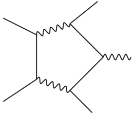
Refer to caption
Figure 1: Massive QED pentagon diagram

Let us consider the one-loop five-point function shown in figure 1. The external momenta fulfill p32=0superscriptsubscript𝑝320p_{3}^{2}=0, pi2=m2superscriptsubscript𝑝𝑖2superscript𝑚2p_{i}^{2}=m^{2} for the other particles, and the sij=(pi+pj)2subscript𝑠𝑖𝑗superscriptsubscript𝑝𝑖subscript𝑝𝑗2s_{ij}=(p_{i}+p_{j})^{2} are kinematical invariants of the process. If we naively use the FUPolynomial function of the MB package, we will get:

U𝑈\displaystyle U =\displaystyle= x1+x2+x3+x4+x5,subscript𝑥1subscript𝑥2subscript𝑥3subscript𝑥4subscript𝑥5\displaystyle x_{1}+x_{2}+x_{3}+x_{4}+x_{5}, (35)
F𝐹\displaystyle F =\displaystyle= m2x12+2m2x1x3s15x1x3+m2x32+2m2x1x4s23x1x4+m2x2x4superscript𝑚2superscriptsubscript𝑥122superscript𝑚2subscript𝑥1subscript𝑥3subscript𝑠15subscript𝑥1subscript𝑥3superscript𝑚2superscriptsubscript𝑥322superscript𝑚2subscript𝑥1subscript𝑥4subscript𝑠23subscript𝑥1subscript𝑥4superscript𝑚2subscript𝑥2subscript𝑥4\displaystyle m^{2}x_{1}^{2}+2m^{2}x_{1}x_{3}-s_{15}x_{1}x_{3}+m^{2}x_{3}^{2}+2m^{2}x_{1}x_{4}-s_{23}x_{1}x_{4}+m^{2}x_{2}x_{4} (36)
\displaystyle- s45x2x4+2m2x3x4+m2x42s12x2x5+m2x3x5s34x3x5.subscript𝑠45subscript𝑥2subscript𝑥42superscript𝑚2subscript𝑥3subscript𝑥4superscript𝑚2superscriptsubscript𝑥42subscript𝑠12subscript𝑥2subscript𝑥5superscript𝑚2subscript𝑥3subscript𝑥5subscript𝑠34subscript𝑥3subscript𝑥5\displaystyle s_{45}x_{2}x_{4}+2m^{2}x_{3}x_{4}+m^{2}x_{4}^{2}-s_{12}x_{2}x_{5}+m^{2}x_{3}x_{5}-s_{34}x_{3}x_{5}.

A simple counting of terms in the F𝐹F-polynomial would prove that this leads to a twelve-dimensional MB-integral. Of course the terms in F𝐹F can be grouped from the beginning and we will see in a minute that a five-fold MB-integral may be obtained; see also the sample file example1.nb222The sample Mathematica files are part of the package AMBRE. They are available at [9, 10]..

First, propagators and kinematical invariants are defined:

Fullintegral[monospace-Fullintegral[\displaystyle\verb#Fullintegral[#
{1},monospace-{1},\displaystyle\verb# {1},#
{PR[k1 + p1, 1, n1]*PR[k1 + p1 + p5, 0, n2]*monospace-{PR[k1 + p1, 1, n1]*PR[k1 + p1 + p5, 0, n2]*\displaystyle\verb# {PR[k1 + p1, 1, n1]*PR[k1 + p1 + p5, 0, n2]*#
PR[k1 + p1 + p4 + p5, 1, n3]*PR[k1 + p1 + p3 + p4 + p5, 1, n4]*monospace-PR[k1 + p1 + p4 + p5, 1, n3]*PR[k1 + p1 + p3 + p4 + p5, 1, n4]*\displaystyle\verb# PR[k1 + p1 + p4 + p5, 1, n3]*PR[k1 + p1 + p3 + p4 + p5, 1, n4]*#
PR[k1 + p1 + p2 + p3 + p4 + p5, 0, n5]},{k1}];monospace-PR[k1 + p1 + p2 + p3 + p4 + p5, 0, n5]},{k1}];\displaystyle\verb# PR[k1 + p1 + p2 + p3 + p4 + p5, 0, n5]},{k1}];# (37)

The kinematics is defined in a cyclic way:

pi2=mi2,si,i+1=(pi+pi+1)2,i=1,,5.formulae-sequencesuperscriptsubscript𝑝𝑖2superscriptsubscript𝑚𝑖2formulae-sequencesubscript𝑠𝑖𝑖1superscriptsubscript𝑝𝑖subscript𝑝𝑖12𝑖15p_{i}^{2}=m_{i}^{2},\qquad s_{i,i+1}=(p_{i}+p_{i+1})^{2},\qquad i=1,...,5. (38)

Then, using the IntPart and SubLoop functions the steps (ii)-(v) of the algorithm (21) are worked out and we end up with a nine-fold MB-representation. This representation is due to the following F𝐹F-polynomial, constructed in the automatic way by AMBRE:

Fsuperscript𝐹\displaystyle F^{{}^{\prime}} =\displaystyle= m2(x1+x3+x4)2s15x1x3s23x1x4+m2x2x4s45x2x4s12x2x5superscript𝑚2superscriptsubscript𝑥1subscript𝑥3subscript𝑥42subscript𝑠15subscript𝑥1subscript𝑥3subscript𝑠23subscript𝑥1subscript𝑥4superscript𝑚2subscript𝑥2subscript𝑥4subscript𝑠45subscript𝑥2subscript𝑥4subscript𝑠12subscript𝑥2subscript𝑥5\displaystyle m^{2}(x_{1}+x_{3}+x_{4})^{2}-s_{15}x_{1}x_{3}-s_{23}x_{1}x_{4}+m^{2}x_{2}x_{4}-s_{45}x_{2}x_{4}-s_{12}x_{2}x_{5} (39)
+m2x3x5s34x3x5.superscript𝑚2subscript𝑥3subscript𝑥5subscript𝑠34subscript𝑥3subscript𝑥5\displaystyle+~{}m^{2}x_{3}x_{5}-s_{34}x_{3}x_{5}.

Some mass terms have been collected here, but the F𝐹F-polynomial can be further simplified by redefining s34s¯34+m2subscript𝑠34subscript¯𝑠34superscript𝑚2s_{34}\to\bar{s}_{34}+m^{2} and s45s¯45+m2subscript𝑠45subscript¯𝑠45superscript𝑚2s_{45}\to\bar{s}_{45}+m^{2}, so that each term xixjsubscript𝑥𝑖subscript𝑥𝑗x_{i}x_{j} appears only once. The Fsuperscript𝐹F^{{}^{\prime}} polynomial becomes finally:

F′′superscript𝐹′′\displaystyle F^{{}^{\prime\prime}} =\displaystyle= m2(x1+x3+x4)2s15x1x3s23x1x4s¯45x2x4s12x2x5s¯34x3x5,superscript𝑚2superscriptsubscript𝑥1subscript𝑥3subscript𝑥42subscript𝑠15subscript𝑥1subscript𝑥3subscript𝑠23subscript𝑥1subscript𝑥4subscript¯𝑠45subscript𝑥2subscript𝑥4subscript𝑠12subscript𝑥2subscript𝑥5subscript¯𝑠34subscript𝑥3subscript𝑥5\displaystyle m^{2}(x_{1}+x_{3}+x_{4})^{2}-s_{15}x_{1}x_{3}-s_{23}x_{1}x_{4}-\bar{s}_{45}x_{2}x_{4}-s_{12}x_{2}x_{5}-\bar{s}_{34}x_{3}x_{5}, (40)

which gives a seven-fold MB-representation. In certain cases, some of the MB-integrations do not depend on the kinematics and Barnes lemmas may be applied. Here, due to the term (x1+x3+x4)2superscriptsubscript𝑥1subscript𝑥3subscript𝑥42(x_{1}+x_{3}+x_{4})^{2} one may twice use Barnes’ first lemma (32) and thus the MB-representation can be further reduced to a five-fold integral. A five-particle scattering process depends on five variables (plus a mass in Bhabha scattering), so a further simplification is impossible.

In sample file example2.nb, we use another definition of kinematical variables, namely

pi2=m2,p1p2=12(t2m2),p1p3=12(ttv1),p1p4=m2+12(v1st),p1p5=12(s2m2),p2p3=12v1,p2p4=12(sv1v22m2),p2p5=12(v2st+2m2),p3p4=12v2,p3p5=12(ttv2),p4p5=12(t2m2),superscriptsubscript𝑝𝑖2superscript𝑚2subscript𝑝1subscript𝑝212superscript𝑡2superscript𝑚2subscript𝑝1subscript𝑝312𝑡superscript𝑡subscript𝑣1subscript𝑝1subscript𝑝4superscript𝑚212subscript𝑣1𝑠𝑡subscript𝑝1subscript𝑝512𝑠2superscript𝑚2subscript𝑝2subscript𝑝312subscript𝑣1subscript𝑝2subscript𝑝412𝑠subscript𝑣1subscript𝑣22superscript𝑚2subscript𝑝2subscript𝑝512subscript𝑣2𝑠superscript𝑡2superscript𝑚2missing-subexpressionsubscript𝑝3subscript𝑝412subscript𝑣2subscript𝑝3subscript𝑝512superscript𝑡𝑡subscript𝑣2subscript𝑝4subscript𝑝512𝑡2superscript𝑚2\begin{array}[]{lll}p_{i}^{2}=m^{2},&p_{1}p_{2}=\frac{1}{2}(t^{\prime}-2m^{2}),&p_{1}p_{3}=\frac{1}{2}(t-t^{\prime}-v_{1}),\\ p_{1}p_{4}=m^{2}+\frac{1}{2}(v_{1}-s-t),&p_{1}p_{5}=\frac{1}{2}(s-2m^{2}),&p_{2}p_{3}=\frac{1}{2}v_{1},\\ p_{2}p_{4}=\frac{1}{2}(s-v_{1}-v_{2}-2m^{2}),&p_{2}p_{5}=\frac{1}{2}(v_{2}-s-t^{\prime}+2m^{2}),&\\ p_{3}p_{4}=\frac{1}{2}v_{2},&p_{3}p_{5}=\frac{1}{2}(t^{\prime}-t-v_{2}),&p_{4}p_{5}=\frac{1}{2}(t-2m^{2}),\end{array} (41)

and we get F𝐹F directly in the form:

F′′′superscript𝐹′′′\displaystyle F^{{}^{\prime\prime\prime}} =\displaystyle= (x1+x3+x4)2tx1x3tx1x4v2x2x4sx2x5v1x3x5.superscriptsubscript𝑥1subscript𝑥3subscript𝑥42𝑡subscript𝑥1subscript𝑥3superscript𝑡subscript𝑥1subscript𝑥4subscript𝑣2subscript𝑥2subscript𝑥4𝑠subscript𝑥2subscript𝑥5subscript𝑣1subscript𝑥3subscript𝑥5\displaystyle(x_{1}+x_{3}+x_{4})^{2}-tx_{1}x_{3}-t^{\prime}x_{1}x_{4}-v_{2}x_{2}x_{4}-sx_{2}x_{5}-v_{1}x_{3}x_{5}. (42)

No wonder, that using function SubLoop we obtain directly the smallest, seven-dimensional integral, which then again reduces to the five-fold integral. The resulting MB-representation for the scalar Feynman integral is:

G[1]𝐺delimited-[]1\displaystyle G[1] =\displaystyle= eεγE(2πi)5i=15i+ui+i+ui𝑑ri(s)3εr1(t)r2(t)r3(v1s)r4(v2s)r5superscript𝑒𝜀subscript𝛾𝐸superscript2𝜋𝑖5superscriptsubscriptproduct𝑖15superscriptsubscript𝑖subscript𝑢𝑖𝑖subscript𝑢𝑖differential-dsubscript𝑟𝑖superscript𝑠3𝜀subscript𝑟1superscript𝑡subscript𝑟2superscriptsuperscript𝑡subscript𝑟3superscriptsubscript𝑣1𝑠subscript𝑟4superscriptsubscript𝑣2𝑠subscript𝑟5\displaystyle\frac{-e^{\varepsilon\gamma_{E}}}{(2\pi i)^{5}}\prod_{i=1}^{5}\int_{-i\infty+u_{i}}^{+i\infty+u_{i}}dr_{i}(-s)^{-3-\varepsilon-r_{1}}(-t)^{r_{2}}(-t^{\prime})^{r_{3}}\left(\frac{v_{1}}{s}\right)^{r_{4}}\left(\frac{v_{2}}{s}\right)^{r_{5}} (43)
Γ[r2]Γ[r3]Γ[1+r2+r3]Γ[r1+r2+r3]Γ[2εr1r4]Γ[r4]Γdelimited-[]subscript𝑟2Γdelimited-[]subscript𝑟3Γdelimited-[]1subscript𝑟2subscript𝑟3Γdelimited-[]subscript𝑟1subscript𝑟2subscript𝑟3Γdelimited-[]2𝜀subscript𝑟1subscript𝑟4Γdelimited-[]subscript𝑟4\displaystyle\Gamma[-r_{2}]\Gamma[-r_{3}]\Gamma[1+r_{2}+r_{3}]\Gamma[-r_{1}+r_{2}+r_{3}]\Gamma[-2-\varepsilon-r_{1}-r_{4}]\Gamma[-r_{4}]
Γ[1+r2+r4]Γ[2εr1r5]Γ[r5]Γ[1+r3+r5]Γdelimited-[]1subscript𝑟2subscript𝑟4Γdelimited-[]2𝜀subscript𝑟1subscript𝑟5Γdelimited-[]subscript𝑟5Γdelimited-[]1subscript𝑟3subscript𝑟5\displaystyle\Gamma[1+r_{2}+r_{4}]\Gamma[-2-\varepsilon-r_{1}-r_{5}]\Gamma[-r_{5}]\Gamma[1+r_{3}+r_{5}]
Γ[3+ε+r1+r4+r5]Γ[3+2r1+r4+r5]Γ[12ε]Γ[3+2(r2+r3)+r4+r5].Γdelimited-[]3𝜀subscript𝑟1subscript𝑟4subscript𝑟5Γdelimited-[]32subscript𝑟1subscript𝑟4subscript𝑟5Γdelimited-[]12𝜀Γdelimited-[]32subscript𝑟2subscript𝑟3subscript𝑟4subscript𝑟5\displaystyle\frac{\Gamma[3+\varepsilon+r_{1}+r_{4}+r_{5}]\Gamma[3+2r_{1}+r_{4}+r_{5}]}{\Gamma[-1-2\varepsilon]\Gamma[3+2(r_{2}+r_{3})+r_{4}+r_{5}]}.

The real parts of the integration strips are 2<u1<12subscript𝑢11-2<u_{1}<-1 and 1/2<ui<0,i=25formulae-sequence12subscript𝑢𝑖0𝑖25-1/2<u_{i}<0,i=2\ldots 5.

A subsequent application of MB shows that up to constant terms in ϵitalic-ϵ\epsilon, needed for an evaluation of two-loop massive Bhabha scattering [11], there are maximally three-dimensional finite contributions to be evaluated further.

4.2 Numerators

AMBRE may handle arbitrary one-loop tensor integrals. The one-loop Feynman parameter integral for a tensor of degree m𝑚m is the generalization of equation (18):

G1(Tm)subscript𝐺1subscript𝑇𝑚\displaystyle G_{1}(T_{m}) \displaystyle\equiv G1(kμ1kμm)subscript𝐺1superscript𝑘subscript𝜇1superscript𝑘subscript𝜇𝑚\displaystyle G_{1}(k^{\mu_{1}}\cdots k^{\mu_{m}})
=\displaystyle= (1)Nνi=1NΓ(νi)i=1Ndxixiνi1δ(1j=1Nxj)r=0mΓ(nd+r2)(2)r2Fnd+r2{𝒜rPmr}[μ1,,μm].superscript1subscript𝑁𝜈superscriptsubscriptproduct𝑖1𝑁Γsubscript𝜈𝑖superscriptsubscriptproduct𝑖1𝑁𝑑subscript𝑥𝑖superscriptsubscript𝑥𝑖subscript𝜈𝑖1𝛿1superscriptsubscript𝑗1𝑁subscript𝑥𝑗superscriptsubscript𝑟0𝑚Γ𝑛𝑑𝑟2superscript2𝑟2superscript𝐹𝑛𝑑𝑟2superscriptsubscript𝒜𝑟superscript𝑃𝑚𝑟subscript𝜇1subscript𝜇𝑚\displaystyle\frac{(-1)^{N_{\nu}}}{\prod_{i=1}^{N}\Gamma(\nu_{i})}\int\prod_{i=1}^{N}dx_{i}x_{i}^{\nu_{i}-1}\delta(1-\sum_{j=1}^{N}x_{j})\sum_{r=0}^{m}\frac{\Gamma\left(n-\frac{d+r}{2}\right)}{(-2)^{\frac{r}{2}}F^{n-\frac{d+r}{2}}}\left\{{\cal A}_{r}P^{m-r}\right\}^{[\mu_{1},\ldots,\mu_{m}]}.

Here FF(x)𝐹𝐹𝑥F\equiv F(x) and PP1(kμ)=ixiPi=i,exiβiepeμ𝑃subscript𝑃1superscript𝑘𝜇subscript𝑖subscript𝑥𝑖subscript𝑃𝑖subscript𝑖𝑒subscript𝑥𝑖subscript𝛽𝑖𝑒superscriptsubscript𝑝𝑒𝜇P\equiv P_{1}(k^{\mu})=\sum_{i}x_{i}P_{i}=\sum_{i,e}x_{i}\beta_{ie}p_{e}^{\mu} were introduced in equations (9) and (17). The r𝑟r starts from zero (with 𝒜0=1subscript𝒜01{\cal A}_{0}=1), and it is 𝒜r=0subscript𝒜𝑟0{\cal A}_{r}=0 for r𝑟r odd, and 𝒜r=g[μi1μi2gμir1μir]{\cal A}_{r}=g^{\left[\mu_{i_{1}}\mu_{i_{2}}\right.}\cdots g^{\left.\mu_{i_{r-1}}\mu_{i_{r}}\right]} for r𝑟r even. The convention [μi1]delimited-[]subscript𝜇subscript𝑖1[\mu_{i_{1}}\ldots] means the totally symmetric combination of the arguments.
In AMBRE tensorial numerators are assumed to be contracted with the external momenta pesubscript𝑝𝑒p_{e}, so that the following quantity is evaluated:

PmG1(Tm)subscript𝑃𝑚subscript𝐺1subscript𝑇𝑚\displaystyle P_{m}~{}G_{1}(T_{m}) \displaystyle\equiv (pe1μ1pemμm)G1(kμ1kμm).superscriptsubscript𝑝subscript𝑒1subscript𝜇1superscriptsubscript𝑝subscript𝑒𝑚subscript𝜇𝑚subscript𝐺1superscript𝑘subscript𝜇1superscript𝑘subscript𝜇𝑚\displaystyle\left(p_{e_{1}}^{\mu_{1}}\cdots p_{e_{m}}^{\mu_{m}}\right)~{}G_{1}(k^{\mu_{1}}\cdots k^{\mu_{m}}). (45)
Refer to caption
Figure 2: Massive QED one-loop box diagram

As an example, we have prepared the massive QED one-loop box of figure 2 in sample file example3.nb with the numerator (k1p1)(k1p2)(k1p3)subscript𝑘1subscript𝑝1subscript𝑘1subscript𝑝2subscript𝑘1subscript𝑝3(k_{1}p_{1})(k_{1}p_{2})(k_{1}p_{3}). The corresponding definition used in AMBRE is:

Fullintegral[monospace-Fullintegral[\displaystyle\verb#Fullintegral[#
{k1*p1,k1*p2,k1*p3},monospace-{k1*p1,k1*p2,k1*p3},\displaystyle\verb# {k1*p1,k1*p2,k1*p3},#
{PR[k1,m,n1]PR[k1+p1,0,n2]PR[k1+p1+p2,m,n3]PR[k1+p3,0,n4]},{k1}];monospace-{PR[k1,m,n1]PR[k1+p1,0,n2]PR[k1+p1+p2,m,n3]PR[k1+p3,0,n4]},{k1}];\displaystyle\verb# {PR[k1,m,n1]PR[k1+p1,0,n2]PR[k1+p1+p2,m,n3]PR[k1+p3,0,n4]},{k1}];#

Obviously, when working with tensor integrals we expect the result to be a sum of several MB-integrals (the higher the rank is, the more integrals will be obtained). We have cross checked numerically results for two-, three- and four-point functions by comparing our results (from using AMBRE and MB) with decompositions of integrals into master integrals using the Integration-By-Parts method implemented in the package IdSolver (M. Czakon, unpublished). Cross checks were done for numerators with up to eight scalar products in the numerators of the Feynman integrals.

Finally we refer to section 5.2 for the interesting special case of irreducible numerators arising in intermediate subloops. In certain cases, the result for a tensor integral may remain as compact as it is for scalar integrals.

4.3 More masses

N𝑁N-point functions with arbitrary internal masses and off-shell external legs give complicated multi-dimensional MB-integrals. Let us consider here and in example4.nb a general one-loop scalar vertex, Fig. 3. In this case we get a five-dimensional MB-integral:

Vgeneralsubscript𝑉general\displaystyle V_{\rm general} =\displaystyle= (1)n123Γ[n1]Γ[n2]Γ[n3]Γ[42εn123]superscript1subscript𝑛123Γdelimited-[]subscript𝑛1Γdelimited-[]subscript𝑛2Γdelimited-[]subscript𝑛3Γdelimited-[]42𝜀subscript𝑛123\displaystyle\frac{(-1)^{n_{123}}}{\Gamma[n_{1}]\Gamma[n_{2}]\Gamma[n_{3}]\Gamma[4-2\varepsilon-n_{123}]} (47)
1(2πi)5i+i𝑑z1i+i𝑑z2i+i𝑑z3i+i𝑑z4i+i𝑑z5i=15Γ[zi]Γ[2ϵn1z1+z5]1superscript2𝜋𝑖5superscriptsubscript𝑖𝑖differential-dsubscript𝑧1superscriptsubscript𝑖𝑖differential-dsubscript𝑧2superscriptsubscript𝑖𝑖differential-dsubscript𝑧3superscriptsubscript𝑖𝑖differential-dsubscript𝑧4superscriptsubscript𝑖𝑖differential-dsubscript𝑧5superscriptsubscriptproduct𝑖15Γdelimited-[]subscript𝑧𝑖Γdelimited-[]2italic-ϵsubscript𝑛1subscript𝑧1subscript𝑧5\displaystyle\frac{1}{(2\pi i)^{5}}\int_{-i\infty}^{+i\infty}dz_{1}\int_{-i\infty}^{+i\infty}dz_{2}\int_{-i\infty}^{+i\infty}dz_{3}\int_{-i\infty}^{+i\infty}dz_{4}\int_{-i\infty}^{+i\infty}dz_{5}\prod_{i=1}^{5}\frac{\Gamma[-z_{i}]}{\Gamma[2-\epsilon-n_{1}-z_{1}+z_{5}]}
(m12)z1(m22)z3(m32)2ϵn123z12345(m12+m22M12)z2(m12+m32M22)z4superscriptsuperscriptsubscript𝑚12subscript𝑧1superscriptsuperscriptsubscript𝑚22subscript𝑧3superscriptsuperscriptsubscript𝑚322italic-ϵsubscript𝑛123subscript𝑧12345superscriptsuperscriptsubscript𝑚12superscriptsubscript𝑚22superscriptsubscript𝑀12subscript𝑧2superscriptsuperscriptsubscript𝑚12superscriptsubscript𝑚32superscriptsubscript𝑀22subscript𝑧4\displaystyle{(m_{1}^{2})}^{z_{1}}{(m_{2}^{2})}^{z_{3}}{(m_{3}^{2})}^{2-\epsilon-n_{123}-z_{12345}}{(m_{1}^{2}+m_{2}^{2}-M_{1}^{2})}^{z_{2}}{(m_{1}^{2}+m_{3}^{2}-M_{2}^{2})}^{z_{4}}
(m22+m32M12M22s)z5Γ[n1+z1124]Γ[42εn1123z1124]superscriptsuperscriptsubscript𝑚22superscriptsubscript𝑚32superscriptsubscript𝑀12superscriptsubscript𝑀22𝑠subscript𝑧5Γdelimited-[]subscript𝑛1subscript𝑧1124Γdelimited-[]42𝜀subscript𝑛1123subscript𝑧1124\displaystyle{(m_{2}^{2}+m_{3}^{2}-M_{1}^{2}-M_{2}^{2}-s)}^{z_{5}}\Gamma[n_{1}+z_{1124}]\Gamma[4-2\varepsilon-n_{1123}-z_{1124}]
Γ[n2+z235]Γ[2+ε+n123+z12345],Γdelimited-[]subscript𝑛2subscript𝑧235Γdelimited-[]2𝜀subscript𝑛123subscript𝑧12345\displaystyle\Gamma[n_{2}+z_{235}]\Gamma[-2+\varepsilon+n_{123}+z_{12345}],

where we abbreviated z1124=2z1+z2+z4subscript𝑧11242subscript𝑧1subscript𝑧2subscript𝑧4z_{1124}=2z_{1}+z_{2}+z_{4} and n123=n1+n2+n3subscript𝑛123subscript𝑛1subscript𝑛2subscript𝑛3n_{123}=n_{1}+n_{2}+n_{3}, etc.

Refer to caption
Figure 3: General one-loop vertex

For the massive QED case, M1=M2=m2=m3=m,m1=0formulae-sequencesubscript𝑀1subscript𝑀2subscript𝑚2subscript𝑚3𝑚subscript𝑚10M_{1}=M_{2}=m_{2}=m_{3}=m,m_{1}=0, we get a compact one-dimensional MB-representation:

VQEDsubscript𝑉QED\displaystyle V_{\rm QED} =\displaystyle= (1)n123Γ[42ϵn1123]Γ[n2]Γ[n3]Γ[42ϵn123]12πii+i𝑑z(m2)z(s)2ϵn123zsuperscript1subscript𝑛123Γdelimited-[]42italic-ϵsubscript𝑛1123Γdelimited-[]subscript𝑛2Γdelimited-[]subscript𝑛3Γdelimited-[]42italic-ϵsubscript𝑛12312𝜋𝑖superscriptsubscript𝑖𝑖differential-d𝑧superscriptsuperscript𝑚2𝑧superscript𝑠2italic-ϵsubscript𝑛123𝑧\displaystyle\frac{(-1)^{n_{123}}\Gamma[4-2\epsilon-n_{1123}]}{\Gamma[n_{2}]\Gamma[n_{3}]\Gamma[4-2\epsilon-n_{123}]}\frac{1}{2\pi i}\int_{-i\infty}^{+i\infty}dz{(m^{2})}^{z}{(-s)}^{2-\epsilon-n_{123}-z} (48)
Γ[z]Γ[2ϵn12z]Γ[2ϵn13z]Γ[2+ϵ+n123+z]Γ[42εn11232z].Γdelimited-[]𝑧Γdelimited-[]2italic-ϵsubscript𝑛12𝑧Γdelimited-[]2italic-ϵsubscript𝑛13𝑧Γdelimited-[]2italic-ϵsubscript𝑛123𝑧Γdelimited-[]42𝜀subscript𝑛11232𝑧\displaystyle\frac{\Gamma[-z]\Gamma[2-\epsilon-n_{12}-z]\Gamma[2-\epsilon-n_{13}-z]\Gamma[-2+\epsilon+n_{123}+z]}{\Gamma[4-2\varepsilon-n_{1123}-2z]}.

4.4 More legs

For topologies with a higher number of legs, there is an increasing number of kinematical invariants and so the dimension of MB-representations increases. The number of dimensions may become smaller after analytical continuation in ε𝜀\varepsilon and for lowest orders in ε𝜀\varepsilon. For a scalar or vector Bhabha massive five-point function, Fig. 1, up to constant terms in ϵitalic-ϵ\epsilon, it includes at most three-dimensional integrals, which hopefully can be solved even analytically [11]. In general, the MB-representation for that case is five-dimensional, see section 1.

In example5.nb we derive MB-representations for a massless and a massive one-loop hexagon scalar diagram, see figure 4. In general, it is an eight-fold integral, but the constant term in ϵitalic-ϵ\epsilon includes again only up to three-dimensional MB-integrals.

If all internal lines have equal non-vanishing mass, one has to deal with a nine-dimensional MB-integral. Again, the numerical results have been checked for both cases in the Euclidean region against sector decomposition. The package contains the auxiliary file
KinematicsGen.m which generates the kinematics for six-point functions with arbitrary off-shell external legs.
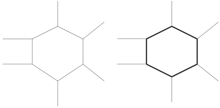
Refer to caption
Figure 4: Six-point scalar functions; left: massless case, right: massive case

5 Multi-loop integrals: loop-by-loop integrations

The Feynman integral (2) includes a delta-function which makes U=1𝑈1U=1 for one-loop diagrams there so that the MB-relation (1) acts only on F𝐹F. This simplification can be made also useful in multi-loop integrals by performing loop-by-loop integrations. We collected few examples which will exhibit several specific features.

5.1 Example: two-loop planar box in massive QED

Let us take the massive two-loop planar box topology333In fact there are three double-box diagrams in massive QED. One of them is non-planar, and we discuss here the so-called first planar diagram [3]. with seven internal lines as introduced in example6.nb. The momentum flow is defined in the following way, with all momenta being incoming:

Fullintegral[monospace-Fullintegral[\displaystyle\verb#Fullintegral[#
{1},monospace-{1},\displaystyle\verb# {1},#
{PR[k1, m, n1]PR[k1 + p1, 0, n2]PR[k1 + p1 + p2, m, n3]monospace-{PR[k1, m, n1]PR[k1 + p1, 0, n2]PR[k1 + p1 + p2, m, n3]\displaystyle\verb# {PR[k1, m, n1]PR[k1 + p1, 0, n2]PR[k1 + p1 + p2, m, n3]#
PR[k1 - k2, 0, n4]PR[k2, m, n5]PR[k2 + p1 + p2, m, n6]monospace-PR[k1 - k2, 0, n4]PR[k2, m, n5]PR[k2 + p1 + p2, m, n6]\displaystyle\verb# PR[k1 - k2, 0, n4]PR[k2, m, n5]PR[k2 + p1 + p2, m, n6]#
PR[k2 - p3, 0, n7]}, {k2, k1}].monospace-PR[k2 - p3, 0, n7]}, {k2, k1}]\displaystyle\verb# PR[k2 - p3, 0, n7]}, {k2, k1}]#. (49)

First, the momentum integration over k2subscript𝑘2k_{2} is taken. The k2subscript𝑘2k_{2} flow in the first subloop is defined by the function IntPart[1], which contains all propagators with momentum k2subscript𝑘2k_{2}:

integral = PR[k1 - k2, 0, n4]*PR[k2, m, n5]*monospace-integral = PR[k1 - k2, 0, n4]*PR[k2, m, n5]*\displaystyle\verb#integral = PR[k1 - k2, 0, n4]*PR[k2, m, n5]*#
PR[k2 + p1 + p2, m,n6]*PR[k2 - p3, 0, n7].monospace-PR[k2 + p1 + p2, m,n6]*PR[k2 - p3, 0, n7]\displaystyle\verb# PR[k2 + p1 + p2, m,n6]*PR[k2 - p3, 0, n7]#. (50)

We just mention that generally it is preferred to choose the order of iteration such that first the loops with lowest number of lines are executed. Then their F𝐹F-polynomials have a minimal number of terms. The first loop’s F𝐹F-polynomial is the SubLoop[integral] function:

Refer to caption
Figure 5: Massive two-loop planar QED box
F[k2]fupc=𝐹delimited-[]subscript𝑘2monospace-fupc=\displaystyle F[k_{2}]\equiv\verb#fupc=#
m^2*FX[X[2] + X[3]]^2 - PR[k1, m]*X[1]*X[2]-monospace-m^2*FX[X[2] + X[3]]^2 - PR[k1, m]*X[1]*X[2]-\displaystyle\verb# m^2*FX[X[2] + X[3]]^2 - PR[k1, m]*X[1]*X[2]-#
PR[k1 + p1 + p2, m]*X[1]*X[3] - s*X[2]*X[3] -monospace-PR[k1 + p1 + p2, m]*X[1]*X[3] - s*X[2]*X[3] -\displaystyle\verb# PR[k1 + p1 + p2, m]*X[1]*X[3] - s*X[2]*X[3] -#
PR[k1 - p3, 0]*X[1]*X[4] + 4*m^2*X[3]*X[4] -monospace-PR[k1 - p3, 0]*X[1]*X[4] + 4*m^2*X[3]*X[4] -\displaystyle\verb# PR[k1 - p3, 0]*X[1]*X[4] + 4*m^2*X[3]*X[4] -#
s*X[3]*X[4] - t*X[3]*X[4] - u*X[3]*X[4]monospace-s*X[3]*X[4] - t*X[3]*X[4] - u*X[3]*X[4]\displaystyle\verb# s*X[3]*X[4] - t*X[3]*X[4] - u*X[3]*X[4]# (51)

It is reproduced here as derived without interactions by the user. The F𝐹F-polnomial contains a mass term with the FX function which later will allow to apply Barnes’ first lemma successfully, and also a redundancy in X[3]*X[4]. The following nine-fold MB-representation after integrating over k2subscript𝑘2k_{2} is obtained:

SubLoop1[((-1))^(n4 + n5 + n6 + n7 + z2 + z3 + z5) 4^z6monospace-SubLoop1[((-1))^(n4 + n5 + n6 + n7 + z2 + z3 + z5) 4^z6\displaystyle\verb#SubLoop1[((-1))^(n4 + n5 + n6 + n7 + z2 + z3 + z5) 4^z6#
(m^2^(z1 + z6) (-s)^(z4 + z7) (-t)^z8monospace-(m^2^(z1 + z6) (-s)^(z4 + z7) (-t)^z8\displaystyle\verb#(m^2^(z1 + z6) (-s)^(z4 + z7) (-t)^z8#
(-u)^(2-ep - n4-n5-n6-n7 - z1 - z2 - z3 - z4 - z5 - z6 - z7 - z8)monospace-(-u)^(2-ep - n4-n5-n6-n7 - z1 - z2 - z3 - z4 - z5 - z6 - z7 - z8)\displaystyle\verb#(-u)^(2-ep - n4-n5-n6-n7 - z1 - z2 - z3 - z4 - z5 - z6 - z7 - z8)#
Gamma[-z1] Gamma[(-z2)] Gamma[(-z3)] Gamma[monospace-Gamma[-z1] Gamma[(-z2)] Gamma[(-z3)] Gamma[\displaystyle\verb#Gamma[-z1] Gamma[(-z2)] Gamma[(-z3)] Gamma[#
2 - ep - n4 - n5 - n6 - z1 - z2 - z3 - z4] Gamma[(-z4)]monospace-2 - ep - n4 - n5 - n6 - z1 - z2 - z3 - z4] Gamma[(-z4)]\displaystyle\verb#2 - ep - n4 - n5 - n6 - z1 - z2 - z3 - z4] Gamma[(-z4)]#
Gamma[(-z5)] Gamma[n4 + z2 + z3 + z5] Gamma[(-z6)] Gamma[(-z7)]monospace-Gamma[(-z5)] Gamma[n4 + z2 + z3 + z5] Gamma[(-z6)] Gamma[(-z7)]\displaystyle\verb#Gamma[(-z5)] Gamma[n4 + z2 + z3 + z5] Gamma[(-z6)] Gamma[(-z7)]#
Gamma[-z8] Gamma[-2+ep + n4 + n5 + n6 + n7 + z1 + z2 + z3 + z4 + z5 +monospace-Gamma[-z8] Gamma[-2+ep + n4 + n5 + n6 + n7 + z1 + z2 + z3 + z4 + z5 +\displaystyle\verb#Gamma[-z8] Gamma[-2+ep + n4 + n5 + n6 + n7 + z1 + z2 + z3 + z4 + z5 +#
z6 + z7 + z8] Gamma[ 2 - ep - n4 - n5 - n7 + z1 - z2 - z5 - z9]monospace-z6 + z7 + z8] Gamma[ 2 - ep - n4 - n5 - n7 + z1 - z2 - z5 - z9]\displaystyle\verb#z6 + z7 + z8] Gamma[ 2 - ep - n4 - n5 - n7 + z1 - z2 - z5 - z9]#
Gamma[(-z9)] Gamma[(-2) z1 + z9] Gamma[n5 + z2 + z4 + z9])/monospace-Gamma[(-z9)] Gamma[(-2) z1 + z9] Gamma[n5 + z2 + z4 + z9])/\displaystyle\verb#Gamma[(-z9)] Gamma[(-2) z1 + z9] Gamma[n5 + z2 + z4 + z9])/#
(Gamma[n4] Gamma[n5] Gamma[n6] Gamma[4 - 2 ep - n4 - n5 - n6 - n7]monospace-(Gamma[n4] Gamma[n5] Gamma[n6] Gamma[4 - 2 ep - n4 - n5 - n6 - n7]\displaystyle\verb#(Gamma[n4] Gamma[n5] Gamma[n6] Gamma[4 - 2 ep - n4 - n5 - n6 - n7]#
Gamma[n7] Gamma[(-2) z1])),monospace-Gamma[n7] Gamma[(-2) z1])),\displaystyle\verb#Gamma[n7] Gamma[(-2) z1])),#
PR[k1, m, z2]PR[k1 + p1 + p2, m, z3]PR[k1 - p3, 0, z5]])monospace-PR[k1, m, z2]PR[k1 + p1 + p2, m, z3]PR[k1 - p3, 0, z5]])\displaystyle\verb#PR[k1, m, z2]PR[k1 + p1 + p2, m, z3]PR[k1 - p3, 0, z5]])# (52)

It is clear that the factors in front of the X[3]X[4] coefficient sum up to zero, due to s+t+u=4m2𝑠𝑡𝑢4superscript𝑚2s+t+u=4m^{2}. To remove them from the beginning, the Fauto[0] option must be executed, followed by a modification of F𝐹F:

fupc = fupc /. u -> 4*m^2-s-t.monospace- fupc = fupc /. u -> 4*m^2-s-t\verb# fupc = fupc /. u -> 4*m^2-s-t#. (53)

In this way, executing the SubLoop[integral] function again, the MB-representation becomes five-dimensional, and also the term 4z6superscript4subscript𝑧64^{z_{6}} is absent now.

The same situation appears in the second iteration, when integrating over k1subscript𝑘1k_{1}. We can switch to the Fauto[0] mode and again modify F𝐹F. After again applying Barnes’ first lemma, we end up with a six-dimensional integral.

Of course, by writing from the very beginning the kinematical invariants without the invariant u𝑢u, one can work out the whole case fully automatic with mode Fauto[1].

5.2 Special numerators

The example6.nb is interesting in yet another respect. After the first integration, the propagators for the second one contain four propagators, some of them with shifted indices compared to the input:

PR[k1, m, n1-z2]PR[k1 + p1, 0, n2]PR[k1 + p1 + p2, m, n3-z3]monospace-PR[k1, m, n1-z2]PR[k1 + p1, 0, n2]PR[k1 + p1 + p2, m, n3-z3]\displaystyle\verb# PR[k1, m, n1-z2]PR[k1 + p1, 0, n2]PR[k1 + p1 + p2, m, n3-z3]#
PR[k1 - p3, 0, z5].monospace-PR[k1 - p3, 0, z5]\displaystyle\verb#PR[k1 - p3, 0, z5]#. (54)

This corresponds to the one-loop box of example example3.nb discussed in section 4.2, but with shifted indices. It includes the one new propagator with momentum q5=k1p3subscript𝑞5subscript𝑘1subscript𝑝3q_{5}=k_{1}-p_{3}. If we would have been evaluating an integral with numerator (q52)n8superscriptsuperscriptsubscript𝑞52subscript𝑛8(q_{5}^{2})^{-n_{8}} and repeat the calculation, we would get after the k2subscript𝑘2k_{2} integral an F𝐹F-polynomial with one of the terms including the propagator PR[k1 + p1 + p2 + p4, 0, 1]; see SubLoop[integral] in example7.nb; see also [5]. It will sum up with PR[k1 + p1 + p2 + p4, 0, -n8] resulting in the following integral

integral= PR[k1, m, n1 - z2] PR[k1 + p1, 0, n2]monospace-integral= PR[k1, m, n1 - z2] PR[k1 + p1, 0, n2]\displaystyle\verb#integral= PR[k1, m, n1 - z2] PR[k1 + p1, 0, n2]#
PR[k1 + p1 + p2, m, n3 - z3]monospace-PR[k1 + p1 + p2, m, n3 - z3]\displaystyle\verb# PR[k1 + p1 + p2, m, n3 - z3]#
PR[k1 + p1 + p2 + p4, 0, -2 + ep + n4 +monospace-PR[k1 + p1 + p2 + p4, 0, -2 + ep + n4 +\displaystyle\verb# PR[k1 + p1 + p2 + p4, 0, -2 + ep + n4 +#
n5 + n6 + n7 - n8 + z1 + z2 + z3 + z4],monospace-n5 + n6 + n7 - n8 + z1 + z2 + z3 + z4]\displaystyle\verb# n5 + n6 + n7 - n8 + z1 + z2 + z3 + z4]#, (55)

which has the following well-known F𝐹F-form of the one-loop box:

m^2 FX[X[1] + X[3]]^2 - s X[1] X[3] - t X[2] X[4].monospace-m^2 FX[X[1] + X[3]]^2 - s X[1] X[3] - t X[2] X[4]\verb#m^2 FX[X[1] + X[3]]^2 - s X[1] X[3] - t X[2] X[4]#.

What is essential here, no additional momentum structure appears.

Analyzing the irreducible numerators of the topology for the given momentum choice, one finds that there are two scalar products which may not be represented by linear combinations of the propagators (and thus are called irreducible): k1p3subscript𝑘1subscript𝑝3k_{1}p_{3} together with k2p1subscript𝑘2subscript𝑝1k_{2}p_{1} or k1p3subscript𝑘1subscript𝑝3k_{1}p_{3} together with k2p2subscript𝑘2subscript𝑝2k_{2}p_{2}. So, q52superscriptsubscript𝑞52q_{5}^{2} represents one of two existing irreducible numerators and it may be quite useful to have a simple MB-representation for that case. We see that there are integrals with (selected) numerators which may be represented by a single MB-representation as if a scalar integral would have been studied. This was used several times in examples given in [5, 6] and in references cited therein, and it was also used e.g. in [12] for a study of massive two-loop box master integrals, and for more sophisticated four-loop cases in [13].

Finally, a six-dimensional MB-integral emerges like in the scalar case. To check this integral numerically with the MB package, two analytical continuations, one in ϵitalic-ϵ\epsilon and one in one of the powers of propagators must be done. We have checked the numerical result also against the results we got from a sector decomposition calculation and from a small-mass expanded version [14, 12].

5.3 Further examples: A three-loop planar box, a four-loop self-energy, and a two-loop pentagon

A three-loop planar integral, shown in figure 6, is treated in example8.nb. The result is a 10-fold MB-representation. With the MB package it was shown that the numerical result agrees with [6].

The dimensions of some MB-representations for several massless and massive ladder topologies are summarized in Table 1. We apply an iterative procedure. For planar topologies the loop-by-loop iteration gives always proper topologies which obey momentum conservation. Only some powers of propagators change into non-integer (complex) numbers.

Massless Massive
1-loop 2-loop 3-loop 4-loop 1-loop 2-loop 3-loop 4-loop
1 4 7 10 3 8 13 18
1 4 7 10 2 6 10 14
Table 1: Dimensions of ladder topologies before and after applying Barnes’ first Lemma.

A similar procedure can be applied to more complicated topologies which obey the same rule: integrating over an internal momentum leads to a topology with propagators and momentum flow obeying momentum conservation in the remaining parts, i.e. we get regular subtopologies.

Refer to caption
Figure 6: The loop-by-loop iterative procedure

In this procedure, the choice of momenta flowing and the order of iterations are very important. Look e.g. at the two-loop ladder example, also shown in figure 6. If we would allow for the momentum flow k1subscript𝑘1k_{1} through all the outer lines, and take first the integration over k1subscript𝑘1k_{1} and then that over k2subscript𝑘2k_{2}, the final representation would not come out optimal (and Barnes’ lemmas do not help). Starting instead with the k2subscript𝑘2k_{2} integration, we will again end up, as with the momentum flows shown in the figure, with a six-dimensional representation.

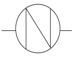
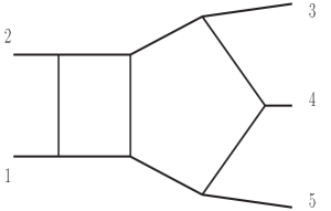
In files example9.nb and example10.nb, massless MB-representations are constructed for a four-loop two-point topology and for a two-loop five-point massless topology, see figure 7. The six-dimensional four-loop self-energy has been checked numerically against sector decomposition. In example10.nb, there are three different derivations of MB-representations for the same kinematics, defined by equation (38). In each case we got another dimension of MB-integrals. The minimal dimension of the integral is seven when we integrate first over internal momenta of the box and then over that of the pentagon. We checked that this agrees numerically with [15] where also a seven-dimensional MB-integral has been obtained. If we integrate first over the internal momentum running in the pentagon and next over that in the box, then a nine-dimensional MB-integral is obtained; again numerically they agree. In the third derivation, the momentum flow in the propagators is chosen in a different way. Then a 13-dimensional MB-integral results.
Refer to caption
Refer to caption
Figure 7: Massless topologies; left: four-loop two-point diagram, right: two-loop five-point diagram

6 Tadpoles

The loop-by-loop approach can also be applied to planar tadpoles. Attention must be paid to keep the right order of integrations. Making iterations with the Fauto[1] option (i.e. automatic), we may end up with three different forms of propagators in the last iteration: one massive propagator, massive and massless propagators, or one massless propagator. For the first situation the well known formula is used in AMBRE:

ddk(k2q2)ν=iπd/2(1)νΓ[ν+ϵ2]Γ[ν]1(q2)ν+ϵ2.superscript𝑑𝑑𝑘superscriptsuperscript𝑘2superscript𝑞2𝜈𝑖superscript𝜋𝑑2superscript1𝜈Γdelimited-[]𝜈italic-ϵ2Γdelimited-[]𝜈1superscriptsuperscript𝑞2𝜈italic-ϵ2\int\frac{d^{d}k}{(k^{2}-q^{2})^{\nu}}=i\pi^{d/2}(-1)^{\nu}\frac{\Gamma[\nu+\epsilon-2]}{\Gamma[\nu]}\frac{1}{(q^{2})^{\nu+\epsilon-2}}. (56)

We found that for some massive tadpoles a term (m)αsuperscript𝑚𝛼(-m)^{\alpha} can appear which would lead to an oscillatory error while doing numerical calculations with MB. In such a situation one has to go back to the previous subloop and modify the F𝐹F-polynomial with Fauto[0] so that two propagators with equal momenta appear: a massive and a massless one. The same procedure must be applied when a single massless propagator appears in the last integral.
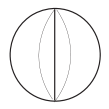
We give as an example example11.nb, for the diagram also shown left in figure 8. Using AMBRE, we have constructed a one-dimensional Mellin-Barnes representation:

T(n1,,n5)𝑇subscript𝑛1subscript𝑛5\displaystyle T(n_{1},...,n_{5}) =\displaystyle= (1)2+n12345(m2)84ϵn123451i=15Γ[ni]Γ[2ϵn4]Γ[2ϵn5]Γ[2ϵ]i+i𝑑z1superscript12subscript𝑛12345superscriptsuperscript𝑚284italic-ϵsubscript𝑛123451superscriptsubscriptproduct𝑖15Γdelimited-[]subscript𝑛𝑖Γdelimited-[]2italic-ϵsubscript𝑛4Γdelimited-[]2italic-ϵsubscript𝑛5Γdelimited-[]2italic-ϵsuperscriptsubscript𝑖𝑖differential-dsubscript𝑧1\displaystyle(-1)^{2+n_{12345}}(m^{2})^{8-4\epsilon-n_{12345}}\frac{1}{\prod_{i=1}^{5}\Gamma[n_{i}]}\frac{\Gamma[2-\epsilon-n_{4}]\Gamma[2-\epsilon-n_{5}]}{\Gamma[2-\epsilon]}\int_{-i\infty}^{+i\infty}dz_{1} (57)
×\displaystyle\times Γ[z1]Γ[2ϵn1z1]Γ[2ϵn2z1]Γ[42ϵn12z1]Γdelimited-[]subscript𝑧1Γdelimited-[]2italic-ϵsubscript𝑛1subscript𝑧1Γdelimited-[]2italic-ϵsubscript𝑛2subscript𝑧1Γdelimited-[]42italic-ϵsubscript𝑛12subscript𝑧1\displaystyle\Gamma[-z_{1}]\Gamma[2-\epsilon-n_{1}-z_{1}]\Gamma[2-\epsilon-n_{2}-z_{1}]\Gamma[4-2\epsilon-n_{12}-z_{1}]
×\displaystyle\times Γ[6+3ϵ+n1245+z1]Γ[8+4ϵ+n12345+z1]Γ[42ϵn122z1]Γdelimited-[]63italic-ϵsubscript𝑛1245subscript𝑧1Γdelimited-[]84italic-ϵsubscript𝑛12345subscript𝑧1Γdelimited-[]42italic-ϵsubscript𝑛122subscript𝑧1\displaystyle\frac{\Gamma[-6+3\epsilon+n_{1245}+z_{1}]\Gamma[-8+4\epsilon+n_{12345}+z_{1}]}{\Gamma[4-2\epsilon-n_{12}-2z_{1}]}

At this point the proper order of integrations is very important. A different choice can lead to two- or even higher-dimensional representations.
Refer to caption
Refer to caption
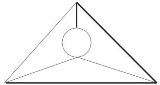
Figure 8: Four-loop tadpoles with three massive lines; left: with a one-dimensional MB-representation, right: with a six-dimensional MB-representation

Using MB we got for the basic integral numerically:

T(1,1,1,1,1)𝑇11111\displaystyle T(1,1,1,1,1) =\displaystyle= 0.25ϵ4+1ϵ3+2.8433003667574471ϵ2+5.7815436104210331ϵ0.25superscriptitalic-ϵ41superscriptitalic-ϵ32.8433003667574471superscriptitalic-ϵ25.7815436104210331italic-ϵ\displaystyle\frac{0.25}{\epsilon^{4}}+\frac{1}{\epsilon^{3}}+2.843300366757447\frac{1}{\epsilon^{2}}+5.781543610421033\frac{1}{\epsilon} (58)
+\displaystyle+ 22.955621881705923+80.89550616785341ϵ+1085.2836587072804ϵ222.95562188170592380.89550616785341italic-ϵ1085.2836587072804superscriptitalic-ϵ2\displaystyle 22.955621881705923+80.89550616785341\epsilon+1085.2836587072804\epsilon^{2}
+\displaystyle+ 4545.303884134432ϵ3+35998.99383263255ϵ4,4545.303884134432superscriptitalic-ϵ335998.99383263255superscriptitalic-ϵ4\displaystyle 4545.303884134432\epsilon^{3}+35998.99383263255\epsilon^{4},

This is in agreement with [16].

However, it appears that MB-representations for four-loop tadpoles can be more complicated. In example12.nb, treating the diagram in figure 8 (right), we get a six-dimensional MB-integral. Taking into account other approaches [16, 17], one may see that the MB-approach to multi-loop calculations has natural limits, especially in the massive cases.

7 On-shell diagrams

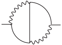
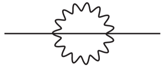
Mellin-Barnes representations can be also useful for solving on-shell topologies. For on-shell self-energies, one may use the package ON-SHELL2 [18, 19] written in FORM v.2.3 [20]. In example13.nb we show how to evaluate the self-energy SE5l3m2 shown in figure 9, which is in the notations of [18] the diagram F01101. The MB-representation is a two-dimensional integral:

F01101F01101\displaystyle{\rm F01101} =\displaystyle= 1(2πi)21Γ[12ϵ]i+i𝑑z1i+i𝑑z2Γ[z1]Γ[z2]Γ[ϵz1]Γ[1+2ϵ+z1]Γ[13ϵz1]1superscript2𝜋𝑖21Γdelimited-[]12italic-ϵsuperscriptsubscript𝑖𝑖differential-dsubscript𝑧1superscriptsubscript𝑖𝑖differential-dsubscript𝑧2Γdelimited-[]subscript𝑧1Γdelimited-[]subscript𝑧2Γdelimited-[]italic-ϵsubscript𝑧1Γdelimited-[]12italic-ϵsubscript𝑧1Γdelimited-[]13italic-ϵsubscript𝑧1\displaystyle-\frac{1}{(2\pi i)^{2}}\frac{1}{\Gamma[1-2\epsilon]}\int_{-i\infty}^{+i\infty}dz_{1}\int_{-i\infty}^{+i\infty}dz_{2}\frac{\Gamma[-z_{1}]\Gamma[-z_{2}]\Gamma[-\epsilon-z_{1}]\Gamma[1+2\epsilon+z_{1}]}{\Gamma[1-3\epsilon-z_{1}]} (59)
×Γ[ϵz1z2]Γ[3ϵz1+z2]Γ[1ϵ+z1+z2]Γ[1+ϵ+z1+z2]Γ[1ϵz1+z2]Γ[2+ϵ+z1+z2].absentΓdelimited-[]italic-ϵsubscript𝑧1subscript𝑧2Γdelimited-[]3italic-ϵsubscript𝑧1subscript𝑧2Γdelimited-[]1italic-ϵsubscript𝑧1subscript𝑧2Γdelimited-[]1italic-ϵsubscript𝑧1subscript𝑧2Γdelimited-[]1italic-ϵsubscript𝑧1subscript𝑧2Γdelimited-[]2italic-ϵsubscript𝑧1subscript𝑧2\displaystyle\times\frac{\Gamma[-\epsilon-z_{1}-z_{2}]\Gamma[-3\epsilon-z_{1}+z_{2}]\Gamma[1-\epsilon+z_{1}+z_{2}]\Gamma[1+\epsilon+z_{1}+z_{2}]}{\Gamma[1-\epsilon-z_{1}+z_{2}]\Gamma[2+\epsilon+z_{1}+z_{2}]}.

In the example, the agreement with the result of On-Shell2 result is demonstrated.

A simpler case is SE3l1m with one massive and two massless propagators, see figure 9. The result is simple:

SE3l1mOS=(m2)(12ϵ)Γ[34ϵ]Γ[1ϵ]2Γ[ϵ]Γ[1+2ϵ]Γ[33ϵ]Γ[22ϵ].SE3l1mOSsuperscriptsuperscript𝑚212italic-ϵΓdelimited-[]34italic-ϵΓsuperscriptdelimited-[]1italic-ϵ2Γdelimited-[]italic-ϵΓdelimited-[]12italic-ϵΓdelimited-[]33italic-ϵΓdelimited-[]22italic-ϵ{\rm SE3l1mOS}=-(m^{2})^{(1-2\epsilon)}\frac{\Gamma[3-4\epsilon]\Gamma[1-\epsilon]^{2}\Gamma[\epsilon]\Gamma[-1+2\epsilon]}{\Gamma[3-3\epsilon]\Gamma[2-2\epsilon]}. (60)

It can be expanded easily to any order in ϵitalic-ϵ\epsilon. Here, in example14.nb, Barnes’ second lemma has been used, which happens not too often. Again, the agreement with the On-Shell2 result is presented.
Refer to caption
Refer to caption
Figure 9: On-shell self-energies; left: SE5l3m2, right: SE3l1m

8 Non-planar topologies

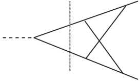
The loop-by-loop iterative procedure described in this paper seems to be not the most efficient approach in the case of non-planar topologies. It is known from [21] that the massless non-planar vertex is described by a two-dimensional Feynman parameter integral. If we consider the loop-by-loop procedure for this case, we can divide the two-loop topology in figure 10 into two parts (follow the vertical line). The hourglass topology on the right-hand side, with two off-shell legs, gives a three-dimensional MB-representation [6], and adding the second part on the left-hand side we end up with a four-dimensional integral. No matter how we arrange the momenta flows in the diagram, it cannot become better. To get the minimal, two-dimensional integral, another approach must be realized. It is an open question to us if the representation of non-planar diagrams can be automatized in a way like that for planar cases444The non-planar examples in the study [7] do not go beyond our observations stated here..
Refer to caption
Figure 10: Non-planar massless vertex

9 Summary

We have described the Mathematica package AMBRE for the construction of MB-representations for planar Feynman integrals and gave in a tutorial part a variety of sample applications. Typically, the iterative loop-by-loop approach gives a possibility to construct MB-integrals of minimal dimension. Usually Barnes’ first and second lemmas help to get the minimal dimension of MB-integrals, independent both of the flow of momenta in diagrams and of the order of iterations. However, for more complicated kinematics, starting with five legs, the order of iterations and the choice of momenta flows matters. As is shown there in the case of tadpoles, MB-representations for massive topologies are not always the best way of evaluation. For some topologies quite simple representations are found, however, also multi-dimensional MB-integrals may arise from which it is hard to get stable, accurate numerical results, not mentioning exact analytical results.

Constructing useful MB-representations for a given Feynman integral is a kind of an art. As an example, let us mention the QED master integral B5l2m2 (a diagram with five lines, two of them being massive; notations are due to [22, 12]). This integral may be obtained by contracting directly two lines in the massive Bhabha two-loop planar integral B7l4m1 [3] (the so-called first planar master of massive QED). In [12] it was shown that, after expansion in ϵitalic-ϵ\epsilon, the expression for B5l2m2 consists of eleven integrals, one being four-dimensional. This was compared to constructing B5l2m2 from the scratch, loop-by-loop. Here, again after expansion in ϵitalic-ϵ\epsilon, we are left with four integrals, all of them being three-dimensional or simpler. This can be checked easily by the reader using the MB package and both the representation B7l4m1 given in [3] (the contraction of two lines must be done there) and the representation B5l2m2 given in [12]. There is no simple relation between both representations, due to our lack of knowledge on more complicated relations between integrals of different dimensionality. One should also mention that an independent check of the MB-representations always is strongly recommended. By construction, neither AMBRE nor MB perform rigorous proofs of their applicability.

Certainly, the number of integration variables is of importance for the final evaluation of MB-integrals, both in a fully analytical form or using approximations in some kinematical limits. In many cases some package like XSUMMER [23, 24] can be used after deriving sums over residua. This again might become non-effective if the number of the nested sums – connected with the dimension of the MB-integrals – is too large or if the result is not in the class of functions covered by (e.g.) XSUMMER. Similar statements hold for the case of a fully numerical evaluation of MB-integrals.

To summarize, for many applications of present phenomenological or more theoretical interest the package AMBRE solves an important part of the complete calculational problem: the derivation of expressions for a large class of Feynman integrals, which may then be used for further study.

Acknowledgments

We would like to thank Sven Moch and Bas Tausk for useful discussions. The development of this package profited very much from a long cooperation with Michal Czakon on NNLO corrections to Bhabha scattering in QED. The present work is supported in part by the European Community’s Marie-Curie Research Training Networks MRTN-CT-2006-035505 ‘HEPTOOLS’ and MRTN-CT-2006-035482 ‘FLAVIAnet’, and by Sonderforschungsbereich/Transregio 9–03 of Deutsche Forschungsgemeinschaft ‘Computergestützte Theoretische Teilchenphysik’.

Appendix A AMBRE functions list

The basic functions of AMBRE are:

  • Fullintegral[{numerator},{propagators},{internal momenta}] – is the basic function for input Feynman integrals

  • invariants – is a list of invariants, e.g. invariants = {p1*p1 \to s}

  • IntPart[iteration] – prepares a subintegral for a given internal momentum by collecting the related numerator, propagators, integration momentum

  • Subloop[integral] – determines for the selected subintegral the U𝑈U and F𝐹F polynomials and an MB-representation

  • ARint[result,i_] – displays the MB-representation number i for Feynman integrals with numerators

  • Fauto[0] – allows user specified modifications of the F𝐹F polynomial fupc

  • BarnesLemma[repr,1,Shifts->True] – function tries to apply Barnes’ first lemma to a given MB-representation; when Shifts->True is set, AMBRE will try a simplifying shift of variables
    BarnesLemma[repr,2,Shifts->True] – function tries to apply Barnes’ second lemma

References

  • [1] V. Smirnov, Phys. Lett. B460 (1999) 397–404, hep-ph/9905323.
  • [2] B. Tausk, Phys. Lett. B469 (1999) 225–234, hep-ph/9909506.
  • [3] V. Smirnov, Phys. Lett. B524 (2002) 129–136, hep-ph/0111160.
  • [4] M. Czakon, J. Gluza, K. Kajda, and T. Riemann, Nucl. Phys. Proc. Suppl. 157 (2006) 16–20, hep-ph/0602102.
  • [5] V. Smirnov, “Evaluating Feynman Integrals” (Springer Verlag, Berlin, 2004).
  • [6] V. Smirnov, “Feynman integral calculus” (Springer Verlag, Berlin, 2006).
  • [7] C. Anastasiou and A. Daleo, JHEP 10 (2006) 031, hep-ph/0511176.
  • [8] M. Czakon, Comput. Phys. Commun. 175 (2006) 559–571, hep-ph/0511200.
  • [9] Katowice, webpage http://prac.us.edu.pl/similar-to\simgluza/ambre.
  • [10] DESY, webpage http://www-zeuthen.desy.de/theory/research/CAS.html.
  • [11] J. Fleischer et al., On pentagon diagrams, to appear.
  • [12] M. Czakon, J. Gluza, and T. Riemann, Nucl. Phys. B751 (2006) 1–17, hep-ph/0604101.
  • [13] Z. Bern, M. Czakon, L. Dixon, D. Kosower, and V. Smirnov, hep-th/0610248.
  • [14] M. Czakon, J. Gluza, and T. Riemann, Nucl. Phys. (Proc. Suppl.) B135 (2004) 83, hep-ph/0406203.
  • [15] Z. Bern, M. Czakon, D. Kosower, R. Roiban, and V. Smirnov, Phys. Rev. Lett. 97 (2006) 181601, hep-th/0604074.
  • [16] R. Boughezal and M. Czakon, Nucl. Phys. B755 (2006) 221–238, hep-ph/0606232.
  • [17] M. Faisst, P. Maierhoefer, and C. Sturm, Nucl. Phys. B766 (2007) 246–268, hep-ph/0611244.
  • [18] J. Fleischer and M. Kalmykov, Comput. Phys. Commun. 128 (2000) 531–549, hep-ph/9907431.
  • [19] M. Kalmykov, webpage http://theor.jinr.ru/similar-to\simkalmykov/onshell2/onshell2.html.
  • [20] J. Vermaseren, “Symbolic manipulation with FORM, Version 2” (Computer Algebra Nederland, Amsterdam, 1991).
  • [21] R. Gonsalves, Phys. Rev. D28 (1983) 1542.
  • [22] M. Czakon, J. Gluza, and T. Riemann, Phys. Rev. D71 (2005) 073009, hep-ph/0412164.
  • [23] S. Moch, P. Uwer, and S. Weinzierl, J. Math. Phys. 43 (2002) 3363–3386, hep-ph/0110083.
  • [24] S. Moch and P. Uwer, Comput. Phys. Commun. 174 (2006) 759–770, math-ph/0508008.