Measuring the dark side (with weak lensing)
Abstract
We introduce a convenient parametrization of dark energy models that is general enough to include several modified gravity models and generalized forms of dark energy. In particular we take into account the linear perturbation growth factor, the anisotropic stress and the modified Poisson equation. We discuss the sensitivity of large scale weak lensing surveys like the proposed DUNE satellite to these parameters. We find that a large-scale weak-lensing tomographic survey is able to easily distinguish the Dvali-Gabadadze-Porrati model from CDM and to determine the perturbation growth index to an absolute error of .
I Introduction
The observed late-time accelerated expansion (e.g. snls ) of the Universe has opened a Pandora’s box in cosmology. Although a great number of models have emerged from the box, none of them has provided a satisfactory explanation of the observations (tsuji and references therein).
In a landscape of hardly compelling theories, probably the most efficient way to proceed is to exploit present and future data in search of signatures of unexpected phenomena that may signal new physical effects. In this way it is possible that we will be able to distinguish, say, a cosmological constant from dynamical dark energy (DE) or the latter from some form of modified gravity.
To this end, an important task is to provide observational groups with simple measurable parameters that may be linked to interesting physics. In this paper we will investigate the extent to which additional parameters can be used to detect signatures of new cosmology in future surveys, with particular emphasis on weak lensing (WL). These additional parameters are connected to the growth of linear perturbations, to the anisotropic stress (defined as the difference bewteen the Newtonian potentials in longitudinal gauge) and to deviations from the Poisson equation for matter. All these parameters find a simple motivation in current models of modified gravity, from extradimensional ones KuSa to scalar-tensor theories; it is clear however that their introduction is not limited to these cases and can in fact account also for other phenomena, for instance clustering in the DE component. We also discuss which of the parameters arise naturally in which context. We then evaluate the sensitivity of WL experiments for two cases: a phenomenological one, in which the parameterization is chosen mainly on the grounds of simplicity and in analogy to some specific models; and a more physically motivated case, namely the Dvali-Gabadadze-Porrati (DGP) dgp extra-dimensional model.
We focus on WL for two reasons: first, contrary to eg supernovae or baryon-oscillation tests, WL makes use of both background and linear perturbation dynamics, allowing to break degeneracies that arise at the background level (this is particularly important for testing modified gravity); second, several groups are planning or proposing large WL experiments in the next decade (e.g. DUNE ; JDEM ; SNAP ) that will reach the sensitivity to test cosmology at unprecedented depth and it is therefore important to optimize the science return of these proposals. We will therefore produce Fisher matrix confidence regions for the relevant parameters for surveys like those proposed by the DUNE DUNE or JDEM/SNAP JDEM ; SNAP collaborations.
The effect of the anisotropic stress has been discussed several times in DE literature. Refs. acqua and ScUzRi discuss it in the context of scalar-tensor theories and evaluated the effect on the shear spectrum; acd discusses its role for a coupled Gauss-Bonnet theory; KuSa showed that it is essential to mimic the DGP growth-rate with a fluid dark energy model; finally, during the final stages of this project another paper discussing the anisotropic stress in dark energy models appeared CaCoMa . Similarly, the parametrization of the growth factor in DE models has been often investigated in the past lahav ; wang .
II Defining the dark Side
In this section we discuss our parametrisation of the dark sector. We separate it into two parts, firstly the parametrisation of the background quantities relevant for a perfectly homogeneous and isotropic universe, and secondly the additional parameters which describe small deviations from this idealised state, at the level of first order perturbation theory.
We assume throughout that the spatial curvature vanishes, mostly for simplicity. We note however that especially in the context of general dark energy models curvature is not yet well constrained ClCoBa .
II.1 Parametrisation of the expansion history
In order to characterise the evolution of the Universe at the background level, we need to provide a parametrisation of the expansion history, . To this end we write it as
| (1) |
We define by the requirement that during matter domination, i.e. at redshifts of a few hundred, the Universe expands according to
| (2) |
We will call this part the (dark) matter, and the remaining part the dark energy. However, these are only effective quantities Kunz . It could be that we are dealing with a tracking dark energy that scales like matter at high redshifts doran ; DTV . In this case, the scaling part of its energy density would be counted as matter. It is also possible that the observed acceleration of the expansion is due to a modification of gravity. In this case there is no dark energy at all and the part takes into account the gravity terms. In all cases, the fundamental quantity is .
The function describes the evolution of the energy density in the (effective) dark energy. The most widely used parametrization makes use of a Taylor series in chevpol ,
| (3) |
where is the scale factor. For the above form of there is an analytic expression of :
| (4) |
However this is not necessarily a good fit to physical models or to the data BaCoKu ; in the DGP case we will make use of the full expression for .
II.2 Parametrisation of the first order quantities
We will limit ourselves to scalar perturbations. In Newtonian gauge we can then write the line element defining the metric as
| (5) |
so that it is characterised by two perturbative quantities, the scalar potentials and .
The perturbations in the dark fluids are characterised for example by their comoving density perturbations and their velocity perturbations . Their evolution is sourced by the potentials and and depends also on the pressure perturbations and the anisotropic stresses of the fluids. For the (dark) matter we set (as in addition this is a gauge-invariant statement) and . In App. A we define our notation and review the perturbation formalism in more detail.
In General Relativity the potential is given by the algebraic relation
| (6) |
which is a generalisation of the Poisson equation of Newtonian gravity (the factor is the spatial Laplacian). We see that in general all fluids with non-zero perturbations will contribute to it. Since we have characterised the split into dark matter and dark energy at the background level, we cannot demand in addition that . At the fluid level, the evolution of is influenced by a combination of the pressure perturbation and the anisotropic stress of the dark energy. However, the pressure perturbation of the dark energy is only very indirectly related to observables through the Einstein equations. For this reason we rewrite Eq. (6) as
| (7) |
where is the gravitational constant measured today in the solar system. Here is a phenomenological quantity that, in general relativity (GR), is due to the contributions of the non-matter fluids (and in this case depends on their and ). But it is more general, as it can describe a change of the gravitational constant due to a modification of gravity (see DGP example below). It could even be apparent: If there is non-clustering early quintessence contributing to the expansion rate after last scattering then we added its contribution to the total energy density during that period wrongly to the dark matter, through the definition of . In this case we will observe less clustering than expected, and we need to be able to model this aspect. This is the role of .
For the dark energy we need to admit an arbitrary anisotropic stress , and we use it to parametrise as
| (8) |
At present there is no sign for a non-vanishing anisotropic stress beyond that generated by the free-streaming of photons and neutrinos. However, it is expected to be non-zero in the case of topological defects KuDu or very generically for modified gravity models KuSa . In most cases, in order to recover the behaviour of the standard model, however in some models like scalar-tensor theories this may not be the case.
If or , then we need to take into account the modified growth of linear perturbations. Defining the logarithmic derivative
| (9) |
it has been shown several times lahav ; wang ; amque ; Linder ; HuLi that for several DE models (including dynamical dark energy and DGP) a good approximation can be obtained assuming
| (10) |
where is a constant that depends on the specific model.
Although for an analysis of actual data it may be preferable to use the parameters , we concentrate in this paper on the use of weak lensing to distinguish between different models. As we will see in the following section, the quantities that enter the weak lensing calculation are the growth index as well as the parameter combination
| (11) |
Weak lensing will therefore most directly constrain these parameters, so that we will use the set for the constraints. Of course we should really think of both as functions of and . An additional benefit of using is that as anticipated it is relatively easy to parametrise since in most models it is reasonable to just take to be a constant (see section III.2). For the situation is however not so clear-cut. First, a simple constant would be completely degenerate with the overall amplitude of the linear matter power spectrum, so would be effectively unobservable per se with WL experiments. Then, even simple models like scalar-tensor theories predict a complicate time-dependence of so that it is not obvious which parametrization is more useful (while for DGP it turns out that just as in GR, see below). So lacking a better motivation we start with a very simple possibility, namely that starts at early times as in GR (i.e. ) and then deviates progressively more as time goes by:
| (12) |
This choice is more general than it seems. If we assume that is linear and equal to unity at some arbitrary , then we have . But since an overall factor can be absorbed into the spectrum normalization, one has in fact where . Therefore, from the error on in (12) one can derive easily the error on the slope at any point .
As a second possibility we also investigate a piece-wise constant function with three different values in three redshift bins. Here again, due to the degeneracy with , we fix .
In this way we have parametrised the three geometric quantities, , and , with the following parameters: , (or ) and , plus those that enter the effective dark energy equation of state. These represent all scalar degrees of freedom to first order in cosmological perturbation theory. The parameterisations themselves are clearly not general, as we have replaced three functions by six or seven numbers, and as we have not provided for a dependence on at all, but they work well for CDM, Quintessence models, DGP and to a more limited extent for scalar-tensor models. We emphasize that this set is optimised for weak lensing forecasts. For the analysis of multiple experiments, one should use a more general parametrisation of and . If the dark energy can be represented as a fluid, then would be another natural choice for the extra degrees of freedom, with and . While phenomenological quantities like , , and are very useful for measuring the behaviour of the dark energy, we see them as a first step to uncovering the physical degrees of freedom. Once determined, they can guide us towards classes of theories – for example would rule out many models where GR is modified.
III Observables
III.1 Constraining the expansion history
In order to constrain the expansion history we can measure either directly or else one of the distance measures. The main tools are
-
•
Luminosity distance: Probed by type-Ia supernova explosions (SN-Ia), this provides currently the main constraints on at low redshifts, .
-
•
Angular diameter distance: Measured through the tangential component of the Baryon Acoustic Oscillations (BAO) either via their imprint in the galaxy distribution sdss_bao or the cosmic microwave background radiation (CMB) wmap3 . One great advantage of this method is the low level of systematic uncertainties. The CMB provides one data point at , while the galaxy BAO probe mostly the range . Using Lyman- observations this could be extended to .
-
•
Direct probes of H(z): This can either be done through the radial component of the BAO in galaxies, or through the dipole of the luminosity distance BoDuKu .
III.2 Growth of matter perturbations
In the standard CDM model of cosmology, the dark matter perturbations on sub-horizon scales grow linearly with the scale factor during matter domination. During radiation domination they grow logarithmically, and also at late times, when the dark energy starts to dominate, their growth is slowed. The growth factor is therefore expected to be constant at early times (but after matter-radiation equality) and to decrease at late times. In addition to this effect which is due to the expansion rate of the universe, there is also the possibility that fluctuations in the dark energy can change the gravitational potentials and so affect the dark matter clustering.
In CDM can be approximated very well through
| (13) |
where . There are two ways that the growth rate can be changed with respect to CDM: Firstly, a general of the dark energy will lead to a different expansion rate, and so to a different Hubble drag. Secondly, if in the Poisson equation (7) we have then this will also affect the growth rate of the dark matter, as will . We therefore expect that is a function of , and .
For standard quintessence models we have and on small scales as the scalar field does not cluster due to a sound speed . In this case is only a weak function of Linder :
| (14) |
A constant turns out to be an excellent approximation also for coupled dark energy models amque and for modified gravity models Linder . A similar change in can also be obtained in models where the effective dark energy clusters KuSa .
If we assume that is the dominant source of the dark matter clustering, then we see that its value is modified by (while the term sourcing perturbations in does not contain the contribution from the anisotropic stress). Following the discussion in LiCa we set
| (15) |
and derive the asymptotic growth index as
| (16) |
In section IV.4 on the DGP model we show how these relations can be inverted to determine and .
Although these relations are useful to gain physical insight and for a rough idea of what to expect, for an actual data analysis one would specify and and then integrate the perturbation equations.
III.3 Weak lensing
Usually it is taken for granted that matter concentrations deflect light. However, the light does not feel the presence of matter, it feels the gravitational field generated by matter. In this paper we consider a scenario where the gravitational field has been modified, so that we have to be somewhat careful when deriving the lensing equations. Following ScUzRi we exploit the fact that it is the lensing potential which describes the deviation of light rays in our scenario. In CDM we can use the Poisson equation (6) to replace the lensing potential with the dark matter perturbations (since the cosmological constant has no perturbations),
| (17) |
However, in general this is not the complete contribution to the lensing potential. For our parametrisation we find instead that
| (18) |
Correspondingly, the total lensing effect is obtained by multiplying the usual equations by a factor . We also notice that a modification of the growth rate appears twice, once in the different behaviour of , and a second time in the non-trivial factor . It is clear that we need to take both into account, using only one of the two would be inconsistent.
An additional complication arises because some of the scales relevant for weak lensing are in the (mildly) non-linear regime of clustering. It is therefore necessary to map the linear power spectrum of into a non-linear one. This is difficult even for pure dark matter, but in this case fitting formulas exist, and numerical tests with -body programs have been performed. For non-standard dark energy models or modified gravity the mapping is not known, and it probably depends on the details of the model. Although this may be used in the long run as an additional test, for now we are left with the question as to how to perform this mapping. In this paper we have decided to assume that represents the effective clustering amplitude, and we use this expression as input to compute the non-linear power spectrum.
One side effect of this prescription is that as anticipated any constant pre-factor of becomes degenerate with (which is also a constant) and cannot be measured with weak lensing. In practice this means that if we use as the fundamental parameters, then a constant contribution to cannot be measured. On the other hand if we use as fundamental parameters then even a constant affects and the degeneracy with is broken through this link.
III.4 Other probes
We have already mentioned one CMB observable, namely the peak position, which is sensitive mostly to the expansion rate of the universe and provides effectively a standard ruler. On large scales the CMB angular power spectrum is dominated by the integrated Sachs-Wolfe (ISW) effect, which is proportional to . The ISW effect therefore probes a similar quantity as weak lensing, but is sensitive to its time evolution. Additionally, it is mostly relevant at low , which means that it is strongly affected by cosmic variance. This limits its statistical power in a fundamental way.
From the perturbation equation for the matter velocity perturbation, Eq. (66) we see that is only sensitive to . Additionally, the peculiar velocities of galaxies are supposed to be a very good tracer of the dark matter velocity field pecvel . The peculiar velocities are therefore a direct probe of alone. This makes it in principle an excellent complement of weak lensing (which measures ) and of the growth rate (measuring mostly through the Poisson equation) but of course measuring reliably peculiar velocities to cosmological distances is still prohibitive.
The perturbations in the metric also affect distance measurements like e.g. the luminosity distance BoDuGa ; HuGr . The fluctuations in the luminosity distance on small angular scales are a measure of both the peculiar motion of the supernovae as well as the lensing by intervening matter perturbations. As very large supernova data sets are expected in the future, this may turn into a promising additional probe of and .
IV Dark energy models
Let us now review some of the models among those presented in the literature that are amenable to our parametrization.
IV.1 Lambda-CDM
In CDM the dark energy contribution to the energy momentum tensor is of the form . From this we see immediately that so that we have a constant . Additionally there are no perturbations in a cosmological constant, which is compatible with the perturbation equations (59) and (60) as they decouple from the gravitational potentials for . For this reason . The absence of off-diagonal terms in the energy momentum tensor also shows that so that . The growth-rate of the matter perturbations is only affected by the accelerated expansion of the universe, with .
IV.2 Quintessence
In quintessence models the dark energy is represented by a scalar field, so that can now vary as a function of time, subject to the condition if . At the level of first order perturbations, quintessence is exactly equivalent to a fluid with and no anisotropic stress (). For such a fluid one often relaxes the condition on , so that becomes allowed (see e.g. KuSa06 and papers cited therein for more details). The high sound speed suppresses clustering on sub-horizon scales so that . It is on these scales that weak lensing and galaxy surveys measure the matter power spectrum, so that , and the growth-rate is only slightly changed through the different expansion rate. From (14) we see that typically one has for the range of still allowed by the data.
On very large scales clustering can be non-negligible, which affects for example the low part of the CMB spectrum through the ISW effect WeLe . For a DGP-like equation of state, we find by integrating the perturbation equations numerically. In general we expect that remains small below the sound horizon, while it can be non-negligible on larger scales. Thus, if we find that on small scales, but for scales larger than some critical scale, then this may be a hint for the existence of a sound horizon of the dark energy. Additionally, one important class of quintessence models exhibits a period of “tracking” at high redshift, during which the energy density in the dark energy stays constant relative to the one in the dark matter doran ; DTV . If the dark energy makes up an important fraction of the total energy density during that period, as defined through Eq. (2) will be too large. In that case as the quintessence clusters less than the dark matter on small scales.
IV.3 A generic dark energy model
A generic non-standard model with either a dark energy very different from quintessence or in which gravity is non-Einsteinian will presumably introduce modifications in the Poisson equation, the equation for dark matter growth and/or the anisotropic stress. Since these quantities are not independent, a generic modified gravity model should allow for at least an additional parameter for and one for . As we anticipated we assume constant and then either or a piece-wise constant in three redshift bins. Let us denote these two “generic dark energy” models as GDE1 and GDE2.
Since these parametrisations contain CDM in their parameter space, which is the phenomenologically most successful model today, they are useful to characterise the sensitivity of experiments to non-standard dark energy models.
IV.4 DGP
An alternative approach to the late-time accelerated expansion of the universe modifies the geometry side of the Einstein equations, rather than the energy content. A well-known model of this kind is the Dvali-Gabadadze-Porrati model dgp . This model is based on five-dimensional gravity, with matter and an additional four-dimensional Einstein-Hilbert action on a brane. This then modifies the evolution of the Universe, with one solution asymptotically approaching a de Sitter universe. Assuming spatial flatness, the Hubble parameter for this solution is given by MaMa
| (19) |
We can solve this quadratic equation for to find
| (20) |
Since the matter stays on the brane, its conservation equation is four-dimensional so that . Considering an effective dark energy component with which leads to the DGP expansion history, one can use the conservation equation to define an effective equation of state with MaMa
| (21) |
For we find and . For we turn to LuScSt ; KoMa which have computed the perturbations on small scales and found
| (22) | |||||
| (23) |
where the parameter is defined as:
| (24) |
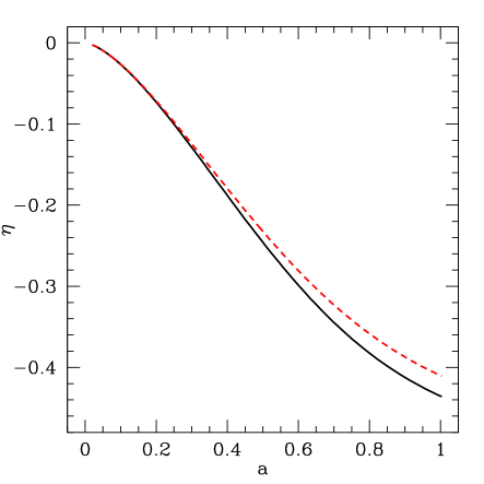
With the parametrisation Eq. (8) we find that
| (25) |
which means that its value today is for . We plot its evolution as a function of in Fig. 1. We see that it vanishes at high redshift, when the modifications of gravity are negligible.
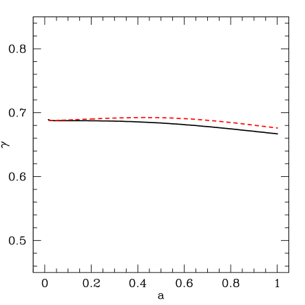
For the growth function we turn to LiCa . They find
| (26) |
Fig. 2 compares this formula with the numerical result, and we see that it works very well. On average in the range we can use .
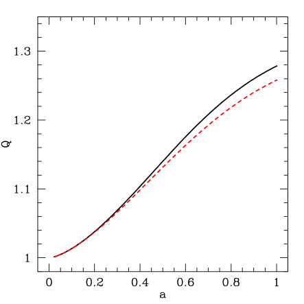
is just the non-trivial pre-factor in Eq. (22),
| (27) |
it is plotted in Figure 3. We find that for DGP so that the deviation of light rays due to a given mass is the same as in GR. The weak lensing results therefore depend only on which modifies the growth of , but not on and separately. In this argument we also used that the gravitational constant measured by a Cavendish type experiment is just the bare constant as the force-law modifications of DGP are screened for LuScSt . This is in contrast to the situation for scalar-tensor theories.
It is maybe instructive to illustrate with a short “Gedanken” experiment how we could recover and from data if our universe was described by a DGP-like model. We assume that has been measured by e.g. supernovae and/or BAO. Suppose now that looking at the growth-history of the matter power spectrum (available potentially as a by-product from a BAO survey or from a dedicated galaxy survey) we notice that is outside the range allowed for quintessence-like models. We therefore have to assume that the dark energy is non-standard. We now need to invert the computation of to get the link with , through the definition of ,
| (28) |
Using the relations in section III.2 we find
| (29) |
Lensing on the other hand gives
| (30) |
For DGP the lensing signal is precisely the one expected naively for , so that
| (31) |
We find that , allowing us to recover and separately. They are shown as the dashed curves in Figs. 1 and 3. Once we know , and we can compute and .
We find that the accuracy of the fitting formula for is quite good, and certainly sufficient for current experiments, and for distinguishing DGP from Quintessence at the perturbation level. We will see later that next-generation weak lensing experiment can reach a precision where the differences are important. At that point one may need to numerically integrate the perturbation equations to compute .
IV.5 DGP
We find it instructive to introduce a simple variant of DGP that we denote as DGP, namely a DGP model which includes a cosmological constant. In this way we can interpolate between DGP proper () and CDM (, ie ). Notice that we are still taking the self-accelerating branch of DGP, different from e.g. LuSt . In flat space, the Hubble parameter is then given by
| (32) |
with the self-accelerating solution now being
| (33) |
In flat space we additionally have that . We also notice that we can define an overall effective dark energy fluid through
| (34) |
from which we can derive an effective equation of state. Concerning the perturbations, it was shown in LuSt that the DGP force laws (22) and (23) are not changed through the addition of a brane cosmological constant if we write as
| (35) |
which depends on the value of . For our key quantities we find
| (36) | |||||
| (37) | |||||
| (38) | |||||
| (39) | |||||
| (40) |
These reduce to the ones of DGP and CDM in the respective limits. The growth factor can be approximated by
| (41) |
where for ease of notation we suppressed the explicit dependence of the s on .
IV.6 Scalar-tensor theories
For completeness we also give a brief overview of the relevant quantities in scalar-tensor theories (see eg. acqua ; ScUzRi ). For a model characterized by the Lagrangian
| (42) |
(where is the coupling function, that we assume to be normalized to unity today and is the bare gravitational constant) the relation between the metric potentials is
| (43) |
where . It turns out that in the linear sub-horizon limit the functions obey three Poisson-like equations:
| (44) | |||||
| (45) | |||||
| (46) |
Then from (28) we derive
| (47) |
where is the presently measured value of the gravitational constant in a Cavendish-like experiment. If the equation (45) can be assumed to hold in the highly non-linear laboratory environment then one would define
| (48) |
Moreover, we obtain the anisotropic stress
| (49) |
Finally, we derive
| (50) |
(notice that our result differs from ScUzRi ). It is clear then that depending on our simple phenomenological parametrization may be acceptable or fail completely. Moreover we find that the usual growth fit (13) is not a very good approximation since during the matter era the growth is faster than in a CDM model. The analysis of specific examples of scalar-tensor models is left to future work.
| Model | growth index | new param. | fid. values | |
|---|---|---|---|---|
| GDE1 | ||||
| GDE2 | ||||
| DGP | ||||
| DGP | or |
V Forecasts for weak lensing large-scale surveys
We finally are in position to derive the sensitivity of typical next-generation tomographic weak lensing surveys to the non-standard parameters introduced above, expanding over recent papers like Refs. jain and taylor . In particular, we study a survey patterned according to the specifications in Ref. amref , which dealt with the standard model. In Appendix B we give the full convergence power spectrum as a function of and and the relevant Fisher matrix equations.
Let us then consider a survey characterized by the sky fraction , the mean redshift and the number sources per arcmin2, . When not otherwise specified we assume and as our benchmark survey: these values are well within the range considered for the DUNE satellite proposal. The derived errors scale clearly as so it is easy to rescale our results to different sky fractions. We assume that the photo- error obeys a normal distribution with variance . We choose to bin the distribution out to into five equal-galaxy-number bins (or three for the model with a piece-wise constant ). For the linear matter power spectrum we adopt the fit by Eisenstein & Hu ehu (with no massive neutrinos and also neglecting any change of the shape of the spectrum for small deviations around ). For the non-linear correction we use the halo model by Smith et al. smith . We consider the range since we find that both smaller and larger ’s do not contribute significantly.
We begin the discussion with the generic dark energy models GDE1 and GDE2. The parameter set (with the fiducial values inside square brackets) is therefore
| (51) |
while for we assume as fiducial values either (GDE1) or (GDE2).
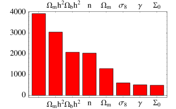
First we study how the estimate of (projection of on the pivot point defined as the epoch at which the errors decorrelate) is affected by fixing the other parameters. In Fig. 4 we show the FOM defined as first when all the parameters are fixed to their fiducial value (first bar) and then successively marginalizing over the parameter indicated in the label and over all those on the left (eg the fourth column represents the marginalization over ). This shows that the WL method would benefit most from complementary experiments that determine . On the other hand, there is not much loss in marginalizing over the two non-standard parameters .
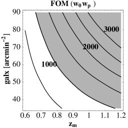
In Fig. 5 we show the confidence regions for . Errors of the order or 0.1 for and 0.3 for are reachable already with the benchmark survey. In Fig. 6 we show the FOM () varying the depth and the density of sources per arcmin2 (full marginalization). If we set as a convenient target a FOM equal to 1000 (for instance, an error of 0.01 for and 0.1 for ) then we see that our benchmark survey remains a little below the target (we obtain and ), which would require at least or a deeper survey.
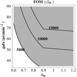
In Fig. 7 we show the FOM () again varying (full marginalization). Here we set as target a FOM of 5000, obtained for instance with an error 0.02 on and on ; it turns out that the target can be reached with the benchmark survey.
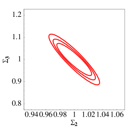
For the model GDE2 we divide the survey into three equal-galaxy-numbers -bins and choose a piece-wise constant in the three bins. Fixing , we are left with two free parameters . In Fig. 8 we show the confidence regions; we see that WL surveys could set stringent limits on the deviation of from the GR fiducial value.
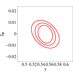
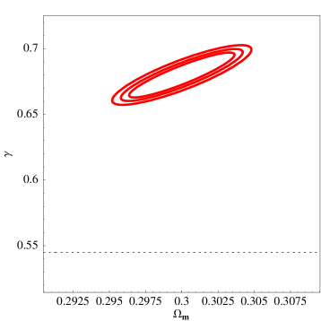
We can now focus our attention to the DGP model. As anticipated, in order to investigate the ability of WL studies to distinguish the DGP model from CDM, we consider two cases. First, we assume a standard DGP model with given by Eq. (21). In this case the model also determines the function . For one has an almost constant in the range with an average value . Instead of using the full equation for we prefer to leave as a free constant parameter in order to compare directly with a standard gravity DE model with the same and the standard value . In Fig. 9 we show the confidence regions around the DGP fiducial model; our benchmark surveys seems well capable of differentiating DGP from CDM.
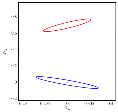
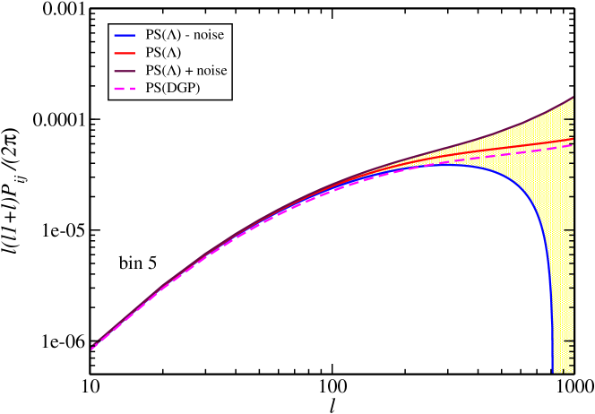
Then, we consider the DGP model, in which the “matter” content is in fact matter plus a cosmological constant, so that in the limit of one recovers DGP, while when one falls back into pure CDM. In Fig. 10 we see again that our benchmark survey will be able to distinguish between the two extreme cases with a very high confidence. In Fig. 11 we display the weak lensing spectrum for CDM in the 5th -bin with the noise due to the intrinsic ellipticity and for comparison the DGP spectrum. We see that the DGP spectrum is well outside the noise at low ’s.
VI Conclusions
In this paper we propose a general parametrisation of both dark energy and modified gravity models up to the linear perturbations. Apart from parametrising the Hubble parameter with an effective equation of state, we use the growth index and the effective modification of the lensing potential . We discuss the relation of these quantities to the anisotropic stress (parametrised through or ) and the modification of the Poisson equation (given in terms of a parameter ). We then show how these parameters appear in different experimental setups, concentrating specifically on the case of weak lensing. We also give explicit expressions for the parameters for a range of models like CDM, Quintessence, the DGP model and scalar-tensor theories. We identify a few signatures that could point to specific theories: The detection of a significant anisotropic stress would favour modified-gravity like theories, while strong upper limits on could rule out many such models. A significant deviation from on large scales only could point to a finite sound speed of the dark energy. The hope is that we can eventually use such clues to understand the physical nature of the phenomenon underlying the accelerated expansion of the Universe.
We use our parametrisation to provide forecasts for weak lensing satellite experiments (having in mind a setup similar to DUNE) on how well they will be able to constrain dark energy and modified gravity models. We find that a DUNE-like survey will be able to constrain the growth index with an error that varies from 0.015 to 0.036 depending on the model (see Table 2). This is sufficient to rule out a model like DGP at more than 7 standard deviations based on the perturbations. Table 2 also shows that the parameter can be strongly constrained. This demonstrates that weak lensing will evolve in the next decade into a very powerful probe of the dark energy phenomenon, with the potential to deliver insight into the physics behind the accelerated expansion of the universe through constraints on the dark energy perturbations and on modified gravity.
| Model | constraints |
|---|---|
| GDE1 | |
| GDE2 | |
| DGP | |
| DGP |
Acknowledgments
MK and DS acknowledge funding from the Swiss NSF. We thank Viviana Acquaviva, Carlo Baccigalupi, Ruth Durrer, Valeria Pettorino and Carlo Schimd for interesting discussions.
Appendix A Perturbation equations
In this appendix we recapitulate the basics of of first order perturbation theory, both to collect the most important equations in one place and to define our notation. We limit ourselves to scalar perturbations, so that we can use the Newtonian gauge (also known as longitudinal gauge), following MaBe . The metric perturbations are then defined by two scalar potentials and ,
| (52) |
The total energy momentum-tensor for a perfect fluid is given by:
| (53) |
where and are the density and the pressure of the fluid respectively and the is the four-velocity. We parametrise the averaged pressure via an equation of state parameter ,
| (54) |
The perturbed energy-momentum tensor in Newtonian gauge can be written as
| (55) | |||||
| (56) | |||||
| (57) |
where can be thought of as the divergence of a velocity field, and , the traceless component of the space-space part of the energy momentum tensor, represents an anisotropic stress. The scalar part of the anisotropic stress is related to through
| (58) |
We additionally introduce a different velocity variable which is better behaved at KuSa06 . In these variables the perturbation equations for the fluids are
| (59) | |||||
| (60) |
where the prime denotes the derivative with respect to the scale factor . The fluid perturbations are all linked by their coupling to the gravitational potentials,
| (61) | |||
| (62) |
where the first equation is a combination of the and Einstein equations of MaBe . It is often convenient to replace the density contrast by the comoving density perturbation,
| (63) |
and the pressure perturbation is often parametrised with the rest-frame sound speed ,
| (64) |
where is the adiabatic sound speed.
As an example, collisionless cold dark matter has zero pressure (), vanishing sound speed and no anisotropic stress . The perturbation equation for the matter fluid then become:
| (65) | |||||
| (66) |
Appendix B The lensing Fisher matrix
Here we discuss how the lensing Fisher matrix is modified in the general case. Let us briefly recall the main equations for weak lensing studies. The convergence weak lensing power spectrum can be written as hujain
| (67) |
where is the non-linear matter power spectrum at redshift obtained correcting the linear power spectrum . In flat space we have:
| (68) | |||||
| (69) | |||||
| (70) | |||||
| (71) | |||||
| (72) |
where is the radial distribution function of galaxies in the -th -bin. We assume an overall radial distribution
| (73) |
The distributions are obtained by binning the overall distribution and convolving with the photo- distribution function.
The Fisher matrix for weak lensing is given by
| (74) |
where the cosmological parameters are and partial derivatives represent , and
| (75) |
where is the rms intrinsic shear (we assume amref ) and
| (76) |
is the number of galaxies per steradians belonging to the -th bin, being the number of galaxies per square arcminute and the fraction of sources belonging to the -th bin.
As we have seen in the main text, we can parametrize a large number of modified gravity models by the linear growth factor and by the combined effect of the modified Poisson equation and the anisotropic stress (the function ). So we have that the convergence spectrum can be written as
| (77) |
where the functions and will in general depend on (and therefore on ) and . Notice moreover that the matter power spectrum depends on the linear growth function which itself is a function of the background expansion and of the functions and .
References
- (1) P. Astier et al, Astron. Astrophys. 447 31 (2006).
- (2) E.J. Copeland, M. Sami and S. Tsujikawa, Int. J. Mod. Phys. D 15 1753 (2006).
- (3) A. Réfrégier et al, astro-ph/0610062 (2006).
- (4) A. Crotts et al, astro-ph/0507043 (2005).
- (5) J. Albert et al, astro-ph/0507460 (2005).
- (6) G.R. Dvali, G. Gabadadze and M. Porrati, Phys. Lett. B 484, 112 (2000).
- (7) R. Caldwell, A. Cooray and A. Melchiorri, astro-ph/0703375
- (8) M. Kunz, astro-ph/0702615 (2007).
- (9) C. Clarkson, M. Cortes and B.A. Bassett, astro-ph/0702670 (2007).
- (10) M. Kunz and D. Sapone, Phys. Rev. Lett 98, 121301 (2007).
- (11) M. Kunz and R. Durrer, Phys. Rev. D 55 4516 (1997).
- (12) R. Maartens and E. Majerotto, Phys. Rev. D 74, 023004 (2006).
- (13) A. Lue, R. Scoccimarro and G.D. Starkmann, Phys. Rev. D 69, 124015 (2004).
- (14) A. Lue and G.D. Starkmann, Phys. Rev. D 70, 101501R (2004).
- (15) K. Koyama, R. Maartens, JCAP 0601, 016 (2006).
- (16) Lahav O. et al. MNRAS 251, 128 (1991)
- (17) L. Wang & P. J. Steinhardt, Astrophys. J. 508, 483 (1998)
- (18) E.V. Linder, Phys. Rev. D 72, 043529 (2005).
- (19) D. Huterer and E.V. Linder, Phys. Rev. D 75, 023519 (2007).
- (20) E.V. Linder and Cahn, astro-ph/0701317 (2007).
- (21) C. Schimd, J.P. Uzan and A. Riazuelo, Phys. Rev. D 71, 083512 (2005).
- (22) T. Padmanabhan, “Structure formation in the universe”, Cambridge University Press (1993).
- (23) C.P. Ma and E. Bertschinger, Astrophys. J. 455, 7 (1995).
- (24) M. Kunz and D. Sapone, Phys. Rev. D 74, 123503 (2006).
- (25) J. Weller and A.M. Lewis, Mon. Not. Roy. Astron. Soc. 346, 987 (2003).
- (26) S.A. Courteau, M.A. Strauss and J.A. Willick, Eds., ASP Conf. Ser. 201, Cosmic Flows (San Francisco: ASP) (2000).
- (27) C. Bonvin, R. Durrer and M.A. Gasparini, Phys. Rev. D 73 023523 (2006).
- (28) C. Bonvin, R. Durrer and M. Kunz, Phys. Rev. Lett. 96, 191302 (2006).
- (29) L. Hui and P.B. Greene, Phys. Rev. D 73 123526 (2006).
- (30) J.P. Uzan, astro-ph/0605313 (2006).
- (31) C. Schimd et al, astro-ph/0603158 (2006).
- (32) D. N. Spergel et al. [WMAP collaboration], astro-ph/0603449 (2006)
- (33) D. Eisenstein et al. [SDSS collaboration] Astrophys. J. 633, 560 (2005) astro-ph/0501171
- (34) V. Acquaviva , Baccigalupi C. & Perrotta F., Phys. Rev. D 70, 3515 (2004)
- (35) L. Amendola & Quercellini C., Phys. Rev. Lett. 92, 181102 (2004)
- (36) L. Amendola, Charmousis C. , Davis S., JCAP 0612, 020 (2006)
- (37) L. Amendola & D. Tocchini-Valentini, Phys. Rev. D 66, 043528 (2002)
- (38) R. Caldwell et al., Astrophys. J. 591, 75 (2003)
- (39) A. Chevallier & Polarski D., IJMPD 10, 213 (2001); Linder, E. V. 2003, Phys. Rev. D 68, 083504 (2003)
- (40) B.A. Bassett, P.S. Corasaniti and M. Kunz, Astrophys. J. 617, L1 (2004)
- (41) W. Hu & B. Jain, astro-ph/0312395
- (42) D. Eisenstein & W. Hu, Astrophys. J. 511, 5 (1999)
- (43) R. E. Smith et al., MNRAS 341, 1311 (2003)
- (44) B. Jain & A. Taylor, Phys Rev. Lett. 91 141302 (2003); M. Ishak, MNRAS 363, 469 (2005); A. Heavens, T. Kitching & A. Taylor, MNARS 373, 105 (2006); A. Taylor et al. MNRAS 374, 1377 (2007)
- (45) A. Amara & A. Réfrégier, astro-ph/0610127
- (46) A. Heavens, T. D. Kitching, L. Verde , astro-ph/0703191