Fundamental Plane of Sunyaev-Zel’dovich clusters

Abstract

Sunyaev-Zel’dovich (SZ) cluster surveys are considered among the most promising methods for probing dark energy up to large redshifts. However, their premise is hinged upon an accurate mass-observable relationship, which could be affected by the (rather poorly understood) physics of the intracluster gas. In this letter, using a semi-analytic model of the intracluster gas that accommodates various theoretical uncertainties, I develop a Fundamental Plane relationship between the observed size, thermal energy, and mass of galaxy clusters. In particular, I find that $M\propto(Y_{SZ}/R_{SZ,2})^{3/4}$, where $M$ is the mass, $Y_{SZ}$ is the total SZ flux or thermal energy, and $R_{SZ,2}$ is the SZ half-light radius of the cluster. I first show that, within this model, using the Fundamental Plane relationship reduces the (systematic+random) errors in mass estimates to $14\%$, from $22\%$ for a simple mass-flux relationship. Since measurement of the cluster sizes is an inevitable part of observing the SZ clusters, the Fundamental Plane relationship can be used to reduce the error of the cluster mass estimates by $\sim 34\%$, improving the accuracy of the resulting cosmological constraints without any extra cost. I then argue why our Fundamental Plane is distinctly different from the virial relationship that one may naively expect between the cluster parameters. Finally, I argue that while including more details of the observed SZ profile cannot significantly improve the accuracy of mass estimates, a better understanding of the impact of non-gravitational heating/cooling processes on the outskirts of the intracluster medium (apart from external calibrations) might be the best way to reduce these errors.

1. Introduction

The origin of the present-day acceleration of the Universe is arguably the most central question in modern cosmology, and is thus likely to dominate theoretical and observational efforts in cosmology for decades to come. As recently highlighted by the Dark Energy Task Force Report (Albrecht et al., 2006), one of the most promising methods for probing the history of cosmic acceleration, or its most likely culprit, Dark Energy, is the abundance of galaxy clusters at large redshifts, which is exponentially sensitive to the cosmic expansion history (Barbosa et al., 1996; Bahcall & Fan, 1998). This has motivated many upcoming cluster surveys such as APEX, ACT, SPT, and SZA, which use the thermal Sunyaev-Zel’dovich (SZ) signature (Sunyaev & Zel’dovich, 1972; Carlstrom et al., 2002) of the hot intracluster gas in the microwave sky to find clusters at high redshifts.

However, the accuracy of any cosmological constraint inferred from a cluster survey is hinged upon how well the mass of the clusters can be estimated from the individual cluster observables. For example, Francis et al. (2005) show that a $10\%$ systematic error in the mass estimates is enough to significantly affect the accuracy of predicted dark energy constraints from upcoming SZ cluster surveys. Although the total SZ flux of a cluster, which traces the total thermal energy of the Intracluster Medium (ICM), is predicted to be a robust tracer of its mass (e.g.,  Birkinshaw, 1999; Carlstrom et al., 2002; Reid & Spergel, 2006), recent X-ray and SZ observations indicate that a significant fraction of cluster baryons may have been removed from the ICM, introducing a new uncertainty into the theoretical predictions (Vikhlinin et al., 2006; Afshordi et al., 2005, 2006; LaRoque et al., 2006; Evrard et al., 2007). Although self-calibration methods, through use of phenomenological/physical ICM models (Majumdar & Mohr, 2004; Younger et al., 2006), clustering of clusters (Lima & Hu, 2004, 2005), or gravitational lensing (Sealfon et al., 2006; Hu et al., 2007) have been put forth as a way to avoid theoretical uncertainties, they do rely on ad hoc power-law fitting formulae and/or modeling assumptions that could jeopardize the accuracy of their applications.

In this letter, I advocate a way to improve the accuracy of mass estimates (or alternatively relax modeling assumptions) through including more information about the observed SZ profile. In particular, while the usual mass estimates only rely on the total SZ flux, I develop a Fundamental Plane relationship (Verde et al., 2002) among the cluster mass, the total SZ flux, and the SZ half-light radius of the cluster. The latter is an independent observable for a moderately resolved cluster, and should be readily measurable at similar precisions to the SZ flux, for the upcoming SZ cluster surveys.

2. Semi-Analytic model of the Intracluster Medium

In order to study the scaling of different ICM observables, we first develop a semi-analytic ICM model which accommodates a generous allowance for different theoretical uncertainties. The main ingredient in our semi-analytic ICM model is the assumption of hot gas sitting in hydrostatic equilibrium in a nearly spherical dark matter halo. The dark matter profile is approximated by an NFW profile (Navarro et al., 1997):

$$\rho(r)=\frac{\rho_{s}}{(r/r_{s})(1+r/r_{s})^{2}},$$ (1)

where $r_{s}$ quantifies the scale at which the slope of the density profile changes from $-1$ to $-3$. This scale is often parameterized using the concentration parameter, $c_{200}=r_{200}/r_{s}$, where $r_{200}$ is the radius within which, the mean density of cluster is $200$ times the critical density of the Universe. We assume a log-normal distribution for $c_{200}$ with the mean:

$$\langle c_{200}\rangle=3.35\left(M_{200}\over 10^{14}h^{-1}M_{\odot}\right)^{-0.11},$$ (2)

and a $22\%$ scatter (Dolag et al., 2004), which is appropriate for an $\Omega_{m}=0.3$ and $\sigma_{8}=0.8$ cosmology (e.g., see Fig. 11 in Mandelbaum et al., 2006). The NFW gravitational potential can then be derived analytically:

$$\phi(r)=-\frac{GM_{200}}{r}\frac{\ln(1+r/r_{s})}{\ln(1+c_{200})-c_{200}/(1+c_{200})}.$$ (3)

Next, we populate this potential with a polytropic gas, i.e. $P_{\rm gas}\propto\rho_{\rm gas}^{\Gamma}$, with $\Gamma\simeq 1.2$ (Suto et al., 1998; Afshordi et al., 2005; Ostriker et al., 2005). Such a polytropic distribution is expected from a turbulent rearrangement and is roughly consistent with hydrodynamical simulations (Ostriker et al., 2005) and X-ray observations (e.g.,  Voit et al., 2003, and references therein). We allow a range

$$1.1<\Gamma<1.3,$$ (4)

with a flat prior, to accommodate uncertainties in and deviations from a polytropic distribution.

In addition to thermal gas pressure, hydrostatic support can be provided by non-thermal sources of pressure. For example, Nagai et al. (2007) show that subsonic turbulent pressure can yield $5\%-20\%$ increase in pressure gradients. Moreover, Pfrommer et al. (2006) argue that cosmic rays can contribute up to $32\%$ of the total pressure in a realistic cluster simulation. To include this uncertainty, we consider a wide range of

$$5\%<\delta_{\rm nth}<50\%,$$ (5)

with a flat prior, where $\delta_{\rm nth}\equiv P_{\rm nth}/P_{\rm gas}$, is the ratio of non-thermal to thermal pressure components

Plugging all sources of pressure into the equation of hydrostatic equilibrium, and using the polytropic relation, we find the ICM temperature profile (e.g.,  Ostriker et al., 2005):

$$T(r)=-\left(\frac{1-\Gamma^{-1}}{1+\delta_{\rm nth}}\right)\left[\phi(r)-\phi(r_{200})\right]+T(r_{200}),$$ (6)

where $T(r_{200})$ is an integration constant, which is proportional to the surface pressure of the region within $r_{200}$. We quantify this constant through the quantity $b^{2}_{T}$ (Evrard et al., 2007), which is defined as:

$$b^{2}_{T}=\frac{\langle T\rangle(<r_{200})}{\mu m_{p}\langle\sigma^{2}_{\rm DM}\rangle(<r_{200})},$$ (7)

where $\langle T\rangle$ is the mean gas mass weighted temperature, $\mu m_{p}$ is the mean particle mass in the ICM plasma ($\mu\simeq 0.59$), and $\langle\sigma^{2}_{\rm DM}\rangle$ is the mean 1D dark matter velocity dispersion. The latter is exquisitely constrained in Evrard et al. (2007) through use of a host of different dark matter simulations:

$$\langle\sigma^{2}_{\rm DM}\rangle^{1/2}(<r_{200})=(1084~{}{\rm km/s})\left(M_{200}\over 10^{15}h^{-1}M_{\odot}\right)^{0.336},$$ (8)

plus $4\%$ random scatter. The ‘Santa Barbara Cluster’ comparison constrains the value of $b^{2}_{T}$ to $0.87\pm 0.04$, for a large range of different adiabatic simulations (Frenk et al., 1999). More recent high resolution simulations that include cooling and feedback effects (Nagai, 2006) yield consistent values

$$b^{2}_{T}=0.90\pm 0.11,$$ (9)

but with larger scatter. We will adopt the latter range with a Gaussian distribution.

In order to set the normalization for the gas pressure/density, we have to fix the total ICM baryonic budget, which we quantify through $f_{\rm gas}\equiv M_{\rm gas}(<r_{200})/M_{200}$. Various X-ray (Vikhlinin et al., 2006; Evrard et al., 2007) and SZ observations (Afshordi et al., 2005, 2006; LaRoque et al., 2006), as well as hydrodynamical simulations (Nagai, 2006) have indicated that $f_{\rm gas}$ may be significantly lower than the total cosmic baryonic budget, which we set to $\Omega_{b}/\Omega_{m}=0.168$ (Spergel et al., 2006). To accommodate this, we also assume a generous range of:

$$0.6<\frac{f_{\rm gas}}{\Omega_{b}/\Omega_{m}}<0.9,$$ (10)

for ICM gas mass fractions.

To estimate the total ICM SZ flux, we need to know the outer edge of our ICM model, or the radius of the accretion shock, $r_{\rm max}$. Assuming that gas comes to stop at the shock, the temperature behind the shock is roughly given by

$$T(r_{\rm max})\simeq\frac{1}{3}\mu m^{2}_{p}v^{2}_{\rm inf.}(1+\delta_{\rm nth})^{-1},$$ (11)

where $v_{\rm inf.}$ is the gas infall velocity. We then use the value of infall velocity from the spherical collapse model (Gunn & Gott, 1972):

$$v_{\rm inf.}=\sqrt{GM(r)\over r}\left\{\sqrt{2}-[2\Delta_{c}]^{-1/3}(Ht/\pi)^{-2/3}+O(\Delta_{c}^{-2/3})\right\},$$ (12)

where $\Delta_{c}$ is the mean overdensity with respect to the critical density within the shock radius. Combining Eqs. (6-7, 11-12) with mean densities from the NFW profile fixes the outer edge of our ICM model.

The final step is to include the ellipticity/triaxiality of real haloes in our model. The impact of triaxiality on the total SZ flux of a halo is of second order, and so we will neglect it in our analysis. However, triaxiality introduces a random scatter in the projected SZ profiles, which will impact the observed half light radii. To model this, we assume that, to first order, the triaxial profile has the shape:

$$P(r,\theta,\varphi)=\bar{P}(r)\left[1+\sum_{m=-2}^{2}a_{2m}Y_{2m}(\theta,\varphi)\right],$$ (13)

where $\bar{P}(r)$ is the prediction from our spherical polytropic model, and $Y_{2m}$’s are spherical harmonics. We then assume a Gaussian distribution with a reasonable range of

$$\langle a^{2}_{2m}\rangle^{1/2}=0.16,\langle a_{2m}\rangle=0,$$ (14)

to model the triaxiality of real clusters. This amplitude of triaxiality has equivalent moments to an ellipsoidal distribution with axes ratios of 1:0.7:0.5 (expected for CDM haloes, e.g.,  Dubinski & Carlberg, 1991), and a (spherically averaged) pressure profile $P(r)\propto r^{-2}$, which is roughly consistent with observations and simulations of SZ clusters (Afshordi et al., 2006).

3. Fundamental Plane of SZ clusters

Let us first quantify the SZ flux of a cluster in terms of $Y_{SZ}$, which we define as

$$Y_{SZ}\equiv{\rm Flux(mK\cdot arcmin^{2})}\left[H(z)d_{A}(z)/c\right]^{2}h^{-1}(z),$$ (15)

where ${\rm Flux(mK\cdot arcmin^{2})}$ is the total observed cluster SZ flux at low frequencies, in units of ${\rm mK\cdot arcmin^{2}}$, while $H(z)=100h(z)~{}{\rm km/s/Mpc}$ and $d_{A}(z)$ are the Hubble constant and the angular diameter distance at redshift $z$. $Y_{SZ}$ can then be easily described in terms of the properties of the ICM model:

$$Y_{SZ}=1.022\left(\frac{M_{\rm gas}h(z)}{10^{15}M_{\odot}}\right)\langle T({\rm keV})\rangle.$$ (16)

Now we can generate a random set of 3000 clusters uniformly distributed in the range

$$13<\log(M_{200}h/M_{\odot})<16,$$ (17)

with their ICM properties according to the prescription that we outlined above . This leads to our mass-SZ flux scaling relation:

$$M_{200}=(8.1\times 10^{14}M_{\odot}/h)~{}Y^{0.58}_{SZ}~{}~{}~{}~{}{\rm(\pm 22\%~{}error)}.$$ (18)

The error quoted here is the r.m.s. scatter around our best fit scaling relation, and reflects a very conservative estimate of all the theoretical uncertainties in mass-SZ flux relation. Also notice that this includes both systematic and random uncertainties, which cannot be distinguished in our approach. A further simplification is the assumed lack of covariance between different uncertainties. While possible constructive/destructive covariances could lead to larger/smaller scatter, their correct account would require a more detailed understanding of the various involved processes.

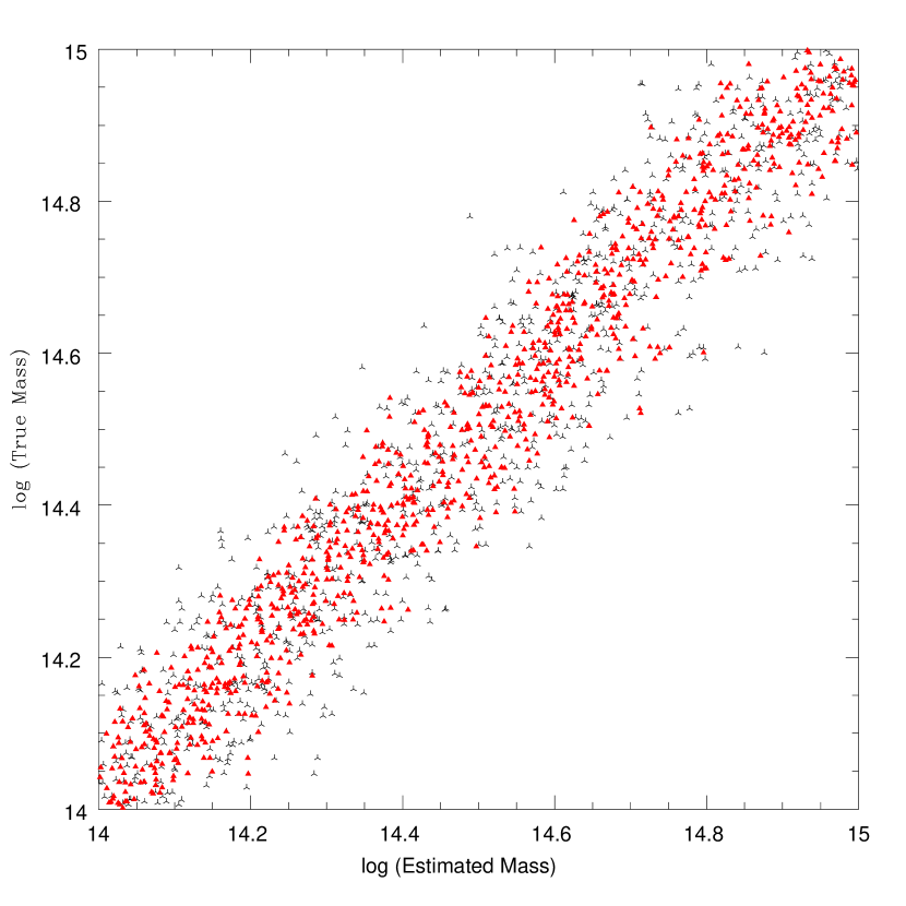
Figure 1.— Contrast between the usual SZ flux mass estimates, Eq. (18), shown by starred (black) points and Fundamental Plane mass estimates, Eq. (19), shown by solid (red) triangle. The error decreases from 22% for the former, to 14% for latter mass estimates.

To approach the main subject of this letter, i.e. the Fundamental Plane of SZ clusters, we will next include information about the ICM SZ profile into our scaling relation. We do this by calculating the half-light radius, $R_{SZ,2}$, which is defined as the radius of the disk (or cylinder) that contains half of the total SZ flux. The new best fit scaling relation for our clusters is:

$$M_{200}=(7.8\times 10^{14}M_{\odot}/h)~{}Y^{0.75}_{SZ}\left(R_{SZ,2}\over{\rm Mpc}/h\right)^{-0.76}$$

$${\rm(\pm 14\%~{}error),}$$ (19)

which shows an almost $34\%$ decrease in the error of the mass estimate. The new scaling relation is shown by solid (red) triangles in Figure (1), which should be contrasted with the starred (black) points that result from the usual mass-SZ flux relation (Eq. 18).

One may wonder if using more information about the SZ profile of the cluster can help reduce the errors in mass estimates even further. To investigate this, we can add the radius of the disk containing a quarter of the total projected SZ flux, $R_{SZ,4}$, into the list of observables. However, we find that the resulting estimator, which now depends on $Y_{SZ}$, $R_{SZ,2}$, and $R_{SZ,4}$, has a scatter of $13\%$, which is almost the same as the error in the Fundamental Plane estimator. Therefore, we conclude that adding more details about the SZ profile is unlikely to improve the accuracy of mass estimates significantly.

4. Physical Origin of the Fundamental Plane

It is interesting to notice that our Fundamental Plane relationship (Eq. 19) is different from the virial relation, $M\propto(Y_{SZ}R_{SZ,2})^{1/2}$, previously adopted e.g., in Verde et al. (2002). The reason for this apparent discrepancy is that the virial relation is only an approximation which results from the assumption of hydrostatic equilibrium and self-similar pressure profiles for different clusters. More specific information about the initial conditions of the cosmological collapse, or the surface pressure, while relaxing the self-similarity assumption, can lead to more accurate scaling relations. Since we use the assumption of hydrostatic equilibrium, most of our clusters sit close to the intersection of the virial relation and Eq. (19), but (by construction) are better fit by Eq. (19).

There is a simple way to understand the physical origin of Eq. (19) analytically. In Sec. 5.1, we show that (within our model) the scatter in the mass-flux relation is dominated by the uncertainty in the surface pressure, which sets the outer boundary of the ICM (Table 1). If we approximate the gravitational potential within the ICM region that dominates the SZ flux by an isothermal potential, and fix all the cluster/ICM parameters, other than its outer boundary, we have $M_{\rm gas}\propto R_{SZ,2}$, while $\langle T_{\rm gas}\rangle\simeq~{}{\rm const}$. Therefore, $Y_{SZ}\propto R_{SZ,2}$ for a fixed cluster potential (and thus fixed $M_{200}$):

$$F(M_{200})=Y_{SZ}/R_{SZ,2}.$$ (20)

Combining this with the standard scaling relations: $Y_{SZ}\propto M^{5/3}_{200}$ and $R_{SZ,2}\propto M_{200}^{1/3}$ yields:

$$M_{200}\propto(Y_{SZ}/R_{SZ,2})^{3/4}.$$ (21)

5. Discussions

5.1. Breakdown of Error Budgets

Table 1 Breakdown of the fractional error in mass estimates into contributions due to different sources of uncertainty.

sources of $\Delta M^{2}/M^{2}$	in Mass-Flux	in Fundamental Plane
halo concentration	0.001	0.003
polytropic index	0.000	0.000
gas fraction	0.004	0.008
non-thermal pressure	0.005	0.004
DM velocity dispersion	0.010	0.005
surface pressure	0.025	0.009
triaxiality	0.000	0.000
total	0.048	0.022

In Table 1, we have broken down the errors in mass estimates into contributions from different sources of uncertainty. To do this for each parameter, we assume that it only takes the central value of its assumed distribution, and then measure the change in the error quadratures of the new scaling relations.

We see that uncertainties in the ICM gas fraction, non-thermal and surface pressures, as well as the dark matter velocity dispersion are the main sources of error in our mass estimates. In contrast, the uncertainties in the halo concentration, the polytropic index, the ICM outer edge, or the halo triaxiality have little impact on the errors.

In particular, the error in both scaling relations seem to be dominated by our assumed uncertainty in the ICM surface pressure, which is ultimately related with the amount of non-gravitational heating/cooling associated with galaxy or black hole formation in the clusters.

Another interesting observation is that the uncertainty in gas fraction has a larger contribution to the error in the Fundamental Plane relation, than to the error in the mass-flux relation. This is due to the fact that $R_{SZ,2}$ does not contain any information about $f_{\rm gas}$ (at least in our model), while Fundamental Plane masses have a steeper dependence on $Y_{SZ}$, and thus are more sensitive to $f_{\rm gas}$ uncertainty.

Notice that possible correlations among different uncertainties, that are overlooked in our simple ICM model, may tilt the Fundamental Plane from our Eq. (1), and also change the size of the errors. However, presence of any such correlations is not immediately obvious in our current theoretical understanding of the ICM physics.

One may wonder why the error in our mass-flux relationship (Eq. 18) is so much larger than those advocated in numerical studies such as Kravtsov et al. (2006), which are only $\sim 6\%$. The reason is that these studies measure the SZ flux within 3D spheres of fixed overdensity ($=500$ times critical, for Kravtsov et al. (2006)), while our total SZ flux is integrated out the ICM accretion shock. Of course, the latter is a more relevant quantity for 2D SZ cluster observations, especially for poor angular resolutions. In fact, our $M_{500}-Y_{SZ,500}$ relation has only a scatter of $9\%$, which is reasonable as we include more theoretical uncertainties than in Kravtsov et al. (2006)’s simulations. This shows that the bulk of the scatter in our mass-flux relationship comes from the uncertainty in the outer edge of our ICM model.

Finally, we should point out that a breakdown into systematic and random errors is also not possible within our exercise, due to our poor statistical understanding of different non-gravitational processes (such as cosmic ray injection or stellar feedback) that affect the scaling relations.

5.2. Noisy Observations

As the purpose of this letter is to introduce a novel and improved mass estimator for SZ cluster surveys, we defer a detailed study of the observational issues associated with the use of this method to future investigation. Such details, while important, should be suited to the specifics of each survey, as well as the class of cosmological models that one would intend to constrain. However, in what follows, I will outline some of the steps that need to be taken for a realistic cosmological application.

We should first recognize that any realistic observation of SZ clusters is limited both by the finite detector noise, as well as the finite beam resolution. While a poor resolution does affect the precision of the SZ flux measurement, its impact is much more severe for the cluster size measurement. For example, if the detector beam is significantly larger than the virial radius of the cluster, then the Fundamental Plane relation cannot add much to the mass-flux relation, even if the cluster is detected at several-$\sigma$ level.

In the absence of perfect resolution, the most practical way to use the Fundamental Plane relation is to fit a parametrized template (e.g., a Gaussian) to the observed cluster SZ map, and replace $R_{SZ,2}$ with the characteristic scale of the template, $\sigma_{SZ}$ . Assuming both Gaussian template and beam, this measurement is done by minimizing the following $\chi^{2}$ function:

$$\chi^{2}=\int\frac{d^{2}\ell}{(2\pi)^{2}}\frac{\left[T_{obs,\vec{\ell}}-Y_{SZ}e^{-\ell^{2}(\sigma^{2}_{SZ}+\sigma^{2}_{\rm beam})/2}\right]^{2}}{C_{\ell}e^{-\ell^{2}\sigma^{2}_{\rm beam}}+N},$$ (22)

where $T_{obs,\vec{\ell}}$ is the flat-sky Fourier transform of the cluster SZ map, $C_{\ell}$ is the CMB power spectrum, $N$ characterizes the detector noise, and $\sigma_{\rm beam}$ is the size of the detector beam.

In the limit that the detector noise is the primary source of measurement uncertainty ($C_{\ell}e^{-\sigma^{2}_{\rm beam}\ell^{2}}\ll N$), the Fisher matrix resulting from Eq. (22) reduces to Gaussian integrals which can be calculated analytically. In particular, for a well-resolved cluster ($\sigma^{2}_{SZ}\mathchar 13350\relax\sigma^{2}_{\rm beam}$), the total (measurement+theory) error in Fundamental Plane masses is only $\sim 28\%(22\%)$ smaller than the SZ-flux mass estimates for a cluster that is detected at a $5\sigma(3\sigma)$ level. This is due to the fact that the theoretical mass degeneracy direction in the $Y_{SZ}-R_{SZ,2}$ (or $Y_{SZ}-\sigma_{SZ}$) plane does not coincide with the degeneracy direction of the measured parameters. Including a finite resolution will only further deteriorate the performance of the Fundamental Plane mass estimates.

6. Conclusions

To summarize, using a semi-analytic model of the intracluster medium which accommodates different theoretical uncertainties, we found a Fundamental Plane relationship that relates the mass of galaxy clusters to their SZ flux and SZ half-light radius. Use of this relationship should lead to $\sim 34\%$ smaller error in mass estimates in comparison to the usual mass-flux relation, and hence more accurate cosmological constraints. While including more details about the SZ profile is unlikely to increase the accuracy of mass estimates, a better understanding of the role of non-gravitational heating/cooling processes should significantly reduce the errors.

While the goal of this letter was to introduce the idea of using Fundamental Plane relationship to improve SZ cluster mass estimates, there is much more that remains to be done in order to exploit the full potential of this method. For example, rather than focusing on the cluster masses, we can study the cosmological constraints from the full bivariate distribution of cluster fluxes and half-light radii $n(Y_{SZ},R_{SZ,2})$. This combines the traditional mass-function constraints, with the constraints resulting from observed scaling relations, as advocated by Verde et al. (2002). Another topic that we did not address here was the impact of including merging (non-relaxed) clusters and/or false detections in our sample. One may identify (and thus exclude) these clusters as outliers in the $Y_{SZ}-R_{SZ,2}$ plane for a given redshift bin, which would not have been possible in the absence of SZ profile information. Finally, it is needless to say that the true Fundamental Plane, as well as the full impact of different theoretical uncertainties, can only be accurately (and adequately) modeled through high-resolution and realistic cosmological simulations of a fair sample of galaxy clusters.

References

- Afshordi et al. (2006) Afshordi, N., Lin, Y.-T., Nagai, D., & Sanderson, A. J. R. 2006, ArXiv Astrophysics e-prints, ADS, astro-ph/0612700
- Afshordi et al. (2005) Afshordi, N., Lin, Y.-T., & Sanderson, A. J. R. 2005, ApJ, 629, 1, ADS, astro-ph/0408560
- Albrecht et al. (2006) Albrecht, A. et al. 2006, ArXiv Astrophysics e-prints, ADS, astro-ph/0609591
- Bahcall & Fan (1998) Bahcall, N. A., & Fan, X. 1998, ApJ, 504, 1, ADS, astro-ph/9803277
- Barbosa et al. (1996) Barbosa, D., Bartlett, J. G., Blanchard, A., & Oukbir, J. 1996, A&A, 314, 13, ADS, arXiv:astro-ph/9511084
- Birkinshaw (1999) Birkinshaw, M. 1999, Phys. Rep., 310, 97, ADS, astro-ph/9808050
- Carlstrom et al. (2002) Carlstrom, J. E., Holder, G. P., & Reese, E. D. 2002, ARA&A, 40, 643, ADS, astro-ph/0208192
- Dolag et al. (2004) Dolag, K., Bartelmann, M., Perrotta, F., Baccigalupi, C., Moscardini, L., Meneghetti, M., & Tormen, G. 2004, A&A, 416, 853, ADS, astro-ph/0309771
- Dubinski & Carlberg (1991) Dubinski, J., & Carlberg, R. G. 1991, ApJ, 378, 496, ADS
- Evrard et al. (2007) Evrard, A. E. et al. 2007, ArXiv Astrophysics e-prints, ADS, astro-ph/0702241
- Francis et al. (2005) Francis, M. R., Bean, R., & Kosowsky, A. 2005, Journal of Cosmology and Astro-Particle Physics, 12, 1, ADS, astro-ph/0511161
- Frenk et al. (1999) Frenk, C. S., et al. 1999, ApJ, 525, 554, ADS, astro-ph/9906160
- Gunn & Gott (1972) Gunn, J. E., & Gott, J. R. I. 1972, ApJ, 176, 1, ADS
- Hu et al. (2007) Hu, W., DeDeo, S., & Vale, C. 2007, ArXiv Astrophysics e-prints, ADS, astro-ph/0701276
- Kravtsov et al. (2006) Kravtsov, A. V., Vikhlinin, A., & Nagai, D. 2006, ApJ, 650, 128, ADS, astro-ph/0603205
- LaRoque et al. (2006) LaRoque, S. J., Bonamente, M., Carlstrom, J. E., Joy, M. K., Nagai, D., Reese, E. D., & Dawson, K. S. 2006, ApJ, 652, 917, ADS, astro-ph/0604039
- Lima & Hu (2004) Lima, M., & Hu, W. 2004, Phys. Rev. D, 70, 043504, ADS, astro-ph/0401559
- Lima & Hu (2005) —. 2005, Phys. Rev. D, 72, 043006, ADS, astro-ph/0503363
- Majumdar & Mohr (2004) Majumdar, S., & Mohr, J. J. 2004, ApJ, 613, 41, ADS, astro-ph/0305341
- Mandelbaum et al. (2006) Mandelbaum, R., Seljak, U., Cool, R. J., Blanton, M., Hirata, C. M., & Brinkmann, J. 2006, MNRAS, 372, 758, ADS, astro-ph/0605476
- Nagai (2006) Nagai, D. 2006, ApJ, 650, 538, ADS, astro-ph/0512208
- Nagai et al. (2007) Nagai, D., Vikhlinin, A., & Kravtsov, A. V. 2007, ApJ, 655, 98, ADS, astro-ph/0609247
- Navarro et al. (1997) Navarro, J. F., Frenk, C. S., & White, S. D. M. 1997, ApJ, 490, 493, ADS
- Ostriker et al. (2005) Ostriker, J. P., Bode, P., & Babul, A. 2005, ApJ, 634, 964, ADS, astro-ph/0504334
- Pfrommer et al. (2006) Pfrommer, C., Ensslin, T. A., Springel, V., Jubelgas, M., & Dolag, K. 2006, ArXiv Astrophysics e-prints, ADS, astro-ph/0611037
- Reid & Spergel (2006) Reid, B. A., & Spergel, D. N. 2006, ApJ, 651, 643, ADS
- Sealfon et al. (2006) Sealfon, C., Verde, L., & Jimenez, R. 2006, ApJ, 649, 118, ADS, astro-ph/0601254
- Spergel et al. (2006) Spergel, D. N., et al. 2006, ArXiv Astrophysics e-prints, ADS, astro-ph/0603449
- Sunyaev & Zel’dovich (1972) Sunyaev, R. A., & Zel’dovich, Y. B. 1972, Comments on Astrophysics and Space Physics, 4, 173, ADS
- Suto et al. (1998) Suto, Y., Sasaki, S., & Makino, N. 1998, ApJ, 509, 544, ADS, astro-ph/9807112
- Verde et al. (2002) Verde, L., Haiman, Z., & Spergel, D. N. 2002, ApJ, 581, 5, ADS, astro-ph/0106315
- Vikhlinin et al. (2006) Vikhlinin, A., Kravtsov, A., Forman, W., Jones, C., Markevitch, M., Murray, S. S., & Van Speybroeck, L. 2006, ApJ, 640, 691, ADS, astro-ph/0507092
- Voit et al. (2003) Voit, G. M., Balogh, M. L., Bower, R. G., Lacey, C. G., & Bryan, G. L. 2003, ApJ, 593, 272, ADS, astro-ph/0304447
- Younger et al. (2006) Younger, J. D., Haiman, Z., Bryan, G. L., & Wang, S. 2006, ApJ, 653, 27, ADS, astro-ph/0605204