Resolving the pulsations of subdwarf B stars: HS 0039+4302, HS 0444+0458, and an examination of the group properties of resolved pulsators

Abstract

We continue our program of single-site observations of pulsating subdwarf B (sdB) stars and present the results of extensive time series photometry of HS 0039+4302 and HS 0444+0458. Both were observed at MDM Observatory during the fall of 2005. We extend the number of known frequencies for HS 0039+4302 from 4 to 14 and discover one additional frequency for HS 0444+0458, bringing the total to three. We perform standard tests to search for multiplet structure, measure amplitude variations, and examine the frequency density to constrain the mode degree $\ell$.

Including the two stars in this paper, 23 pulsating sdB stars have received follow-up observations designed to decipher their pulsation spectra. It is worth an examination of what has been detected. We compare and contrast the frequency content in terms of richness and range and the amplitudes with regards to variability and diversity. We use this information to examine observational correlations with the proposed $\kappa$ pulsation mechanism as well as alternative theories.

1 Introduction

Subdwarf B (sdB) stars are horizontal-branch stars with masses $\approx 0.5M_{\odot}$, thin ($<10^{-2}M_{\odot}$) hydrogen shells, and temperatures from $22\,000$ to $40\,000$ K (Heber, 1984; Saffer et al., 1994). Pulsating sdB stars come in two varieties: short period (90 to 600 seconds), and long period (45 minutes to 2 hours). This work concentrates on the short-period pulsators, which are named EC 14026-2647 stars after the prototype (Kilkenny et al., 1997); they are also known as V361 Hya stars or sdBV stars. They typically have pulsation amplitudes near 1%, and detailed studies reveal a few to dozens of frequencies. The longer period pulsators are known as PG 1716 pulsators after that prototype and typically have amplitudes less then 0.1% (Green et al., 2003). They are also cooler then the EC 14026-type pulsators, though there is some overlap, and they are most likely $g-$mode pulsators (Fontaine et al., 2006).

Asteroseismology of pulsating sdB stars can potentially probe the interior structure and provide estimates of total mass, shell mass, luminosity, helium fusion cross sections, and coefficients for radiative levitation and gravitational diffusion. To apply the tools of asteroseismology, however, it is necessary to resolve the pulsation frequencies. This usually requires extensive photometric campaigns, preferably at several sites spaced in longitude to reduce day/night aliasing. Generally, discovery surveys have simply identified variables and detected only the highest-amplitude pulsations, while multisite campaigns have observed few sdBV stars.

We have been engaged in a long-term program to resolve poorly-studied sdB pulsators, principally from single-site data. This method has proven useful for several sdBV stars (Reed et al., 2004, 2006a, 2007; Zhou et al., 2006). Here, we report the results of our observations of HS 0039+4302 (hereafter HS 0039) and HS 0444+0458 (hereafter HS 0444). HS 0039 ($B=15.6$) and HS 0444 ($B=16.5$) were discovered to be members of the EC 14026 class by Østensen et al. (2001, hereafter Ø01). Their observations of HS 0039 consisted of three runs of 1, 2, and 3 hours, and they obtained three $\approx 1.5$ hour runs for HS 0444. Even with these short runs, they were able to detect four frequencies in HS 0039 and two in HS 0444. Ø01 also obtained spectra of both stars, from which they determined $T_{\rm eff}=33~{}100$ K and $34~{}500$ K, and $\log g=6.0$ and $6.1$ (with $g$ in cgs units of $cm\cdot s^{-2}$) for HS 0039 and HS 0444, respectively, and that neither star is a spectroscopic binary. In §2 we describe our new observations of these stars, in §3 we analyze the pulsation frequencies, and in §4 we discuss our findings and apply asteroseismic tests.

With the addition of these two stars, 23 sdBV stars have received follow-up observations, including 18 stars for which our program has directly contributed data. In §5, we will discuss the observational properties of all 23 stars, concentrating on pulsation stability, amplitudes, and a comparison with known driving mechanisms.

2 Observations

Data were obtained at MDM Observatory’s 1.3 m telescope using an Apogee Alta U47+ CCD camera. MDM Observatory is located on the southwest ridge of Kitt Peak, Arizona and is operated by a consortium of five universities, including the Ohio State University. Images were transferred via USB2.0 for high-speed readout; our binned ($2\times 2$) images had an average dead-time of one second. The observations used a red cut-off filter (BG38), so the effective bandpass covers the $B$ and $V$ filters and is essentially that of a blue-sensitive photomultiplier tube. Such a setup allows us to maximize light throughput while maintaining compatibility with observations obtained with photomultipliers. Tables 1 and 2 provide the details of our observations including date, start time, run length, and integration time. The observations total nearly 100 hours of data for HS 0039 and more than 60 hours for HS 0444.

Standard image reduction procedures, including bias subtraction, dark current and flat field correction, were followed using IRAF packages. Intensities were extracted using aperture photometry. Extinction and cloud corrections were obtained from the normalized intensities of several field stars. Because sdB stars are substantially hotter than typical field stars, differential light curves are not flat due to atmospheric reddening. A low-order polynomial was fit to remove nightly trends from the data. Finally, the lightcurves were normalized by their average flux and centered around zero so the reported differential intensities are $\Delta I=\left(I/\langle I\rangle\right)-1$. Amplitudes are given as milli-modulation amplitudes (mma), with 10 mma corresponding to 1.0% or 9.2 millimagnitudes. Sample lightcurves are shown in Fig. 1.

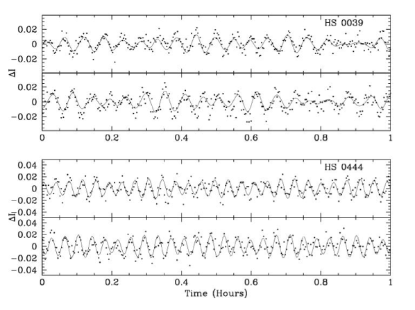
Figure 1: Representative lightcurves of HS 0039 (top pair) and HS 0444 (bottom pair). Each panel is one hour in length. The line shows our fit to the data. Note that the vertical scale differs for the two plots.

Table 1: Observations of HS 0039

Run	UT Start	UT Date	Length	Integration
	(h:m:s)	2005	(hr)	(s)
mdm111505	01:46:00	15 Nov.	7.9	15
mdm111605	01:17:00	16 Nov.	8.4	12
mdm111705	01:18:00	17 Nov.	8.4	12
mdm111805	01:16:00	18 Nov.	8.5	12
mdm111905	01:15:00	19 Nov.	8.5	12
mdm112005	01:23:00	20 Nov.	8.3	12
mdm112105	01:23:00	21 Nov.	8.2	10
mdm112205	01:11:00	22 Nov.	8.6	10
mdm112505	02:35:00	25 Nov.	6.5	12
mdm112605	01:06:00	26 Nov.	4.0	12
mdm112705	01:11:00	27 Nov.	0.6	12
mdm112805	01:11:00	28 Nov.	6.2	10
mdm112905	01:06:00	29 Nov.	6.4	10
mdm113005	01:90:00	30 Nov.	3.4	10
mdm120905	01:24:00	09 Dec.	4.7	8
mdm121405	01:14:00	14 Dec.	1.1	8

Table 2: Observations of HS 0444

Run	UT Start	UT Date	Length	Integration
	(h:m:s)	2005	(hr)	(s)
hs04mdm111505	09:54:00	15 Nov.	3.0	15
hs04mdm111605	09:52:00	16 Nov.	3.1	12
hs04mdm111705	09:53:00	17 Nov.	3.0	12
hs04mdm111805	09:52:00	18 Nov.	2.9	12
hs04mdm111905	09:53:00	19 Nov.	2.8	12
hs04mdm112005	09:57:00	20 Nov.	2.7	12
hs04mdm112105	09:48:00	21 Nov.	2.8	12
hs04mdm112205	10:52:00	22 Nov.	1.6	12
hs04mdm112605	05:26:00	26 Nov.	6.8	12
hs04mdm112705	08:59:00	27 Nov.	3.1	12
hs04mdm112805	07:23:10	28 Nov.	4.8	10
hs04mdm112905	07:32:00	29 Nov.	4.5	10
hs04mdm113005	04:26:00	30 Nov.	4.7	10
hs04mdm120905	06:26:40	09 Dec.	2.6	15
hs04mdm121005	01:30:30	10 Dec.	9.5	10
hs04mdm121405	05:45:10	14 Dec.	5.3	12

3 Pulsation Analysis

HS 0039: A quick analysis during observations alerted us that the amplitudes of HS 0039 were not stable. This is easily seen in the final nightly reductions, twelve of which are shown in Fig. 2. In this figure, we show the pulsation spectra (Fourier transforms; FTs) from adjacent nights, except for the short night on 27 November. Only the frequency near 4270 $\mu$Hz appears stable in amplitude, while those near 5175, 5482, and 7348 $\mu$Hz show substantial variation. We therefore examined the amplitudes and phases for indications of closely spaced multiplets, which would produce roughly sinusoidal amplitude variations and phase changes near the median amplitude (see Daszyńska-Daszkiewicz et al., 2005). Figure 3 shows our non-linear least-squares fits for the four dominant frequencies.

Figure 2: Pulsation spectra of temporally adjacent data runs for HS 0039 plotted at the same scale.

The frequency near 4270 $\mu$Hz is the most stable, both in amplitude and phase. The remaining three frequencies show significant amplitude variation, but only a little variation in phase. The phase for the peak near 5175 $\mu$Hz shows an unusual bimodality at the beginning of the campaign, with a steady, intermediate value at the end. We therefore separated the data into two subsets composed of data from the first seven runs (15 – 21 Nov.) and the last six runs (25 – 30 Nov.). Figure 4 shows the region near 5175 $\mu$Hz for all the November data and the two subsets. The FT of the first seven runs allowed us to interpret the phase information: the frequency at 5175 $\mu$Hz is composed of a close doublet separated by $\sim 17\mu$Hz. The separation between frequencies is just shorter than 1 day ($11.6$ $\mu$Hz) and so nightly runs will not resolve these into two separate frequencies. Evidently the timing was just right near the beginning of the campaign that the phase switched between the two frequencies of the doublet on alternate nights. This was not the case later in the run, although the very last phase might show that the pattern was reestablishing itself.

Figure 3: Amplitudes and phases of the four largest amplitude frequencies of HS 0039. Frequencies are provided (in $\mu$Hz) in each panel.

Figure 4: Close-up of the region near 5175 $\mu$Hz showing prewhitening of the frequency doublet in HS 0039. From top to bottom the panels are the window functions, the original FTs, and the FTs prewhitened by one, and two frequencies. The left panels are the complete data, the middle panels are the first seven data runs combined, and the right panels are the last six data runs combined.

The frequency near 5482 $\mu$Hz shows a similar variation in amplitude to that near 5175 $\mu$Hz, but not the bimodal phase. We grouped the data into the same subsets as in Fig. 4, but did not see any clear sign of a close doublet. If the amplitude variations were intrinsic to that peak, the discovery of frequencies by prewhitening would be more complicated. We produced an accurate window function as in Reed et al. (2006a); the window function is the FT of a noise-free sinusoidal single frequency sampled at the same times as the data. The window function matched the multi-peaked structure of the temporal spectra around 5482 $\mu$Hz, leading us to conclude that the amplitude and phase variations are intrinsic to that frequency and it is not a closely-spaced multiplet. We also examined the region near 7348 $\mu$Hz in the complete data and in the subsets. There is no indication of closely spaced multiplets, nor in the the phases (Fig. 3). We conclude that this frequency also has intrinsic amplitude variations, but is a temporally resolved frequency.

We do not see any such indications in the remaining frequencies, though most have amplitudes that are too small to be detected in individual runs. Armed with five resolved frequencies, we continued simultaneously least-squares fitting and removing peaks (prewhitening) in the combined data set. This process is shown in Fig. 5, where the top panel is the original FT and the next three panels show residuals after prewhitening by 5, 10, and 14 frequencies (from top to bottom). The solid (blue in the on-line version) line in the figure indicates the $4\sigma$ noise limit, below which we do not fit any peaks. After fitting 14 frequencies, we concluded that any remaining power in the residuals was caused by amplitude and/or phase variations and so does not represent remaining unfit frequencies. The solution to our fit, listing frequencies, periods, and average amplitudes is provided in Table 3.

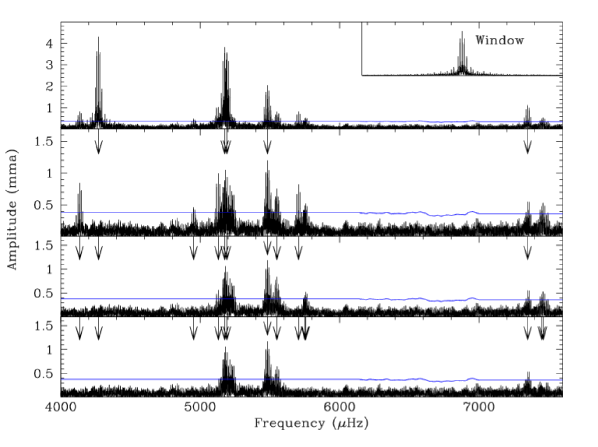
Figure 5: Temporal spectrum for the complete HS 0039 data set showing the prewhitening sequence. The top panel shows the original FT while the remaining panels show the data prewhitened by 5, 10, and 14 frequencies, respectively. The prewhitened frequencies are indicated by arrows and the solid (blue in the on-line version) lines indicate the $4\sigma$ detection level while the inset is the window function.

Table 3: Frequencies, periods, and average amplitudes for HS 0039. Formal least-squares errors are in parentheses.

ID	Frequency	Period	Amplitude
	($\mu$Hz)	(s)	(mma)
$f1$	4135.559 (0.042)	241.8052 (0.0024)	0.85 (0.09)
$f2$	4271.481 (0.008)	234.1108 (0.0004)	4.35 (0.09)
$f3$	4952.858 (0.078)	201.9035 (0.0031)	0.46 (0.09)
$f4$	5130.474 (0.036)	194.9137 (0.0013)	1.00 (0.09)
$f5$	5175.466 (0.009)	193.2193 (0.0003)	3.99 (0.09)
$f6$	5192.660 (0.010)	192.5794 (0.0003)	3.73 (0.09)
$f7$	5482.319 (0.016)	182.4045 (0.0005)	2.16 (0.09)
$f8$	5550.170 (0.047)	180.1746 (0.0015)	0.77 (0.09)
$f9$	5705.677 (0.044)	175.2640 (0.0013)	0.82 (0.09)
$f10$	5751.316 (0.081)	173.8732 (0.0024)	0.45 (0.09)
$f11$	5756.651 (0.068)	173.7120 (0.0020)	0.53 (0.09)
$f12$	7348.444 (0.031)	136.0832 (0.0006)	1.15 (0.09)
$f13$	7449.256 (0.064)	134.2415 (0.0011)	0.65 (0.09)
$f14$	7459.765 (0.063)	134.0524 (0.0011)	0.67 (0.09)

HS 0444: Early in our campaign, we concentrated on HS 0039, leaving HS 0444 as a secondary target. Even from the relatively short runs (Table 2), we could tell that HS 0444 was a simple pulsator with just a few frequencies. In December, when HS 0444 was better placed in the sky, we obtained longer individual runs to ensure that we did not miss any low amplitude peaks. The temporal spectrum of HS 0444 is shown in Fig. 6. The top panel shows the original FT, the bottom panel the residuals after prewhitening by three frequencies, and the inset is the window function. The frequencies, periods and amplitudes from our least-squares solution are provided in Table 4. In Fig. 7, we show the amplitudes and phases of the two frequencies which were detectable each night. The amplitudes and phases are relatively stable and do not show any indications of additional unresolved frequencies.

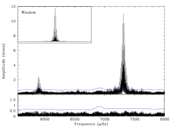
Figure 6: Temporal spectra for HS 0444. The top panel shows the original FT, the bottom the residuals after prewhitening by three frequencies, and the inset is the window function. The solid (blue) line is the $4\sigma$ detection limit.

Table 4: Periods, frequencies, and amplitudes for HS 0444. Formal least-squares errors are in parentheses.

ID	Frequency	Period	Amplitude
	($\mu$Hz)	(s)	(mma)
$f1$	5902.511 (0.012)	169.41940 (0.00035)	2.5 (0.2)
$f2$	6553.484 (0.037)	152.59056 (0.00086)	0.8 (0.2)
$f3$	7311.728 (0.003)	136.76657 (0.00005)	11.1 (0.2)

Figure 7: Amplitudes and phases for frequencies $f1$ and $f3$ of HS 0444.

4 Discussion

4.1 Comparison with the discovery data

The goal of our observational program is to resolve the pulsation frequencies for asteroseismic analysis. For the sake of comparison with the discovery data, we calculate the temporal resolution as $1/\Delta t$ with $\Delta t$ being the extent of the observations in time (see Kilkenny et al., 1999). For the discovery data, we can determine the temporal resolution from information provided in Ø01, and estimate the detection limit as twice the top of the noise level in their FTs outside of the pulsations and window functions.

For HS 0039, our observations have a temporal resolution of 0.8 $\mu$Hz (excluding the December runs), which is $\approx 6.5\times$ better than the discovery data. The detection limit is 0.4 mma, which is about $5\times$ better than in Ø01. It is difficult to determine whether the frequencies in HS 0039 have changed since the discovery observations. Ø01’s reported frequencies (5.14, 5.48, and 4.27 mHz) roughly correspond to our $f4$ or $f5$, $f7$, and $f2$, respectively, but Ø01’s last frequency of 5.21 mHz, detected in only a single observing run, is not found in our data. As this frequency is wedged between higher-amplitude frequencies, and Ø01’s window function is complex, it is difficult to judge the significance of its detection, though it does look reasonable in their figures. However, the main difficulty is the abundance of frequencies, many of which have low amplitudes. The discovery data only detected four frequencies, whereas we detect 14. We estimate Ø01’s noise limit as $\approx 2$ mma; if our limit were as high, we also would have detected four frequencies. It is therefore not possible to ascertain the long-term stability of the pulsations from just these two sets of data.

Additional data on HS 0039 were obtained using the ULTRACAM multicolor instrument on the 4.2 m William Herschel Telescope in 2002 by Jeffery et al. (2004; hereafter J04). Two long ($\approx 8$ hr) runs with very high signal-to-noise were obtained on consecutive nights. We recover J04’s eight frequency detections, six of which are independent. Two are aliases of $f7$ and one is an alias of $f13$. J04 used multicolour photometry to estimate that $f8$ is an $\ell=4$ mode. Though geometric cancellation should reduce amplitudes for higher degree modes, the $(\ell,m)=(4,1)$ mode can be reduced by as little as 30%, depending on orientation (Reed et al., 2005). Since $f8$ is 18% the amplitude of $f2$ (the highest amplitude frequency), there is no problem in ascribing it as an $\ell=4$ mode. Additionally, as this region of the FT is relatively uncrowded, the data obtained by J04 should have been sufficient to make this determination. Although they do not claim this identification with certainty, it seems reasonable and would certainly be worth additional multicolour photometry or time-series spectroscopy for confirmation.

For HS 0444, our observations have a temporal resolution of 0.4 $\mu$Hz, which is $\approx 14\times$ better than the discovery data. The detection limit is 0.6 mma, which is about $3\times$ better than in Ø01. Additionally, we have recovered the two frequencies detected in the discovery data, to within the errors, and uncover a single new frequency, at an amplitude below their detection limit.

4.2 Constraints on the pulsation modes

In addition to improving the known pulsation spectra of these stars, we wish to place observational constraints on the pulsation modes. The modes are mathematically described by spherical harmonics with three quantum numbers, $n$ (or $k$), $\ell$, and $m$. Rotation can break the $m$ degeneracy by separating each degree $\ell$ into a multiplet of $2\ell+1$ components, so multiplet structure is a very useful tool for observationally constraining pulsation degree (see Winget et al., 1991; Reed et al., 2004; O’Toole et al., 2004).

For slow rotators, like most sdB stars are thought to be (Heber, Reid, Werner, 1999, 2000), rotationally-split multiplets should be nearly equally spaced in frequency. Such structure is, however, seldom observed in sdBV stars and in neither case are multiplets detected in our observations. Even though HS 0039 has 14 frequencies, the frequency spacings are not regular. Instead, the spacings are distributed from 5 to 3325 $\mu$Hz, with no obvious groupings. For HS 0444, there are only three detected frequencies, but the spacings are not similar, so there is no multiplet structure in this star.

Another tool that can be used is the density of frequencies within a given range. In resolved sdBV stars, we sometimes observe many more pulsation modes than $\ell=0$, 1, and 2 can provide, independent of the number of inferred $m\neq 0$ frequencies. Higher $\ell$ modes may be needed, but if so they must have a larger amplitude than is measured because of the large degree of geometric cancellation (Charpinet et al., 2005; Reed et al., 2005). A general guideline would be one $n$ order per $\ell$ degree per 1000 $\mu$Hz (Charpinet et al. (2002) find an average spacing near 1440 $\mu$Hz), so the temporal spectrum can accommodate three frequencies per 1000 $\mu$Hz without the necessity of invoking high-$\ell$ values if no multiplet structure is observed. Filling all possible $m$ values, the limit becomes nine frequencies per 1000 $\mu$Hz..

Obviously there is no need to invoke high-$\ell$ modes for HS 0044. Between 4900 and 5800 $\mu$Hz, HS 0039 has 9 of its 14 frequencies. Therefore, HS 0039 has too large a frequency density to exclude $\ell\geq 3$ modes, particularly with the absence of any obvious multiplets. This supports the identification of an $\ell=4$ mode by J04.

5 Group Properties

5.1 Data sources

Since the discovery of the EC 14026 class of pulsating sdB stars in 1997 (Kilkenny et al., 1997), there have been three areas of emphasis for observations: 1) to discover more pulsators; 2) to resolve the pulsations using long time-base campaigns, sometimes at multiple sites; and 3) to obtain high signal-to-noise observations over short time intervals. In recent years, multicolour photometry and time-series spectroscopy have been obtained as additional tools for mode identification.

For this paper, we will concentrate on the second point above, and examine pulsators for which a considerable effort has been expended to resolve the pulsation frequencies. We do this because it has been our area of emphasis, we feel that it is an important component in applying asteroseismology to sdB stars, and most importantly, we have data for all the stars except those from Kilkenny et al. (2002, 2006a, 2006b). Though this will not be a complete sample of sdBV follow-up observations, we can perform uniform tests upon them (except as noted above) for intercomparison.

Table 5 provides a list of studies that have thoroughly investigated the pulsations of sdBV stars. Some stars, such as Feige 48, PG 0014, PG 1219, and PG 1605, have received extensive observations over the course of many years, while most have only been observed during a single campaign. Column 1 of that table lists the full name of each pulsator. Columns 2 and 3 display the dates of observations and the number of hours observed. The final two columns display the observing sites and references for each star. The references in Table 5 are the basis for our analysis below, but are not necessarily a complete record of the detailed observations of each star.

Table 5: List of follow-up observations of pulsating sdB stars. A dagger^† indicates observations that we were involved in and NA indicates information that was not available. Observing sites: 1) Suhora 0.6 m; 2) Baker 0.4 m; 3) CTIO 1.5 m; 4) SAAO 1.9 m; 5) Fick 0.6 m; 6) MDM 1.3 m; 7) McDonald 2.1 m; 8) McDonald 0.9 m; 9) MDM 2.4 m; 10) Whole Earth Telescope Campaign, 11) Multisite campaign by Reed et al., 12) Other campaign. Column 5 references are: a) Baran et al. 2005; b) Reed et al. 2006b; c) Kilkenny et al. 2006a; d) Kilkenny et al. 2006b; e) Reed et al. 2004; f) this work; g) Reed et al. 2006a; h) Silvotti et al. 2002a; i) Reed et al. 2006c; j) Zhou et al. 2006; k) O’Donoghue et al. 1998a; l) Vuc̆ković et al. 2006; m) Reed et al. 2007; n) Kilkenny et al. 2002; o) Harms, Reed, O’Toole 2006; p) Silvotti et al. 2006; q) Kilkenny et al. 2003; r) Kilkenny et al. 1999; U) unpublished.

Target	Inclusive Dates	Hours Observed	Sites	References
Balloon090100001	17 Aug. - 19 Sep. 2004	125	1	a
†	8 Aug. - 30 Sep. 2005	NA	2, 12	U
EC 05217-3914†	6 - 15 Nov. 1999	59	3, 4	b
EC 14026-2647	July 2003	NA	4	c
EC 20338-1925	23 Jul. - 26 Sep., 1998	45.9	4	d
	June 2004 (2 nights)	12	4	c
Feige 48†	1998 – 2006	$>500$	2, 5, 6, 7, 8, 10, 11	e
HS 0039+4302†	15 Nov. - 14 Dec. 2005	91	6	f
HS 0444+0458†	15 Nov. - 14 Dec. 2005	63	6	f
HS 1824+5745†	25 May - 11 Jul. 2005	127	6, 9	g
HS 2149+0847	July 2003 (4 nights)	NA	4	d
	June 2004 (10 nights)	NA	4	d
HS 2151+0857†	18 Jun. - 11 Jul. 2005	42	6, 9	g
HS 2201+2610†	17 Sep. - 4 Oct. 2000	95.0	5, 12	h
KPD 1930+2752†	11 - 16 Jul. 2002	38	7, 11	i
†	15 Aug. - 9 Sep. 2003	246.5	10	U
KPD 2109+4401†	12 Sep. - 14 Oct. 2004	182.6	2, 6, 11	j
PB 8783	8 - 22 Oct. 1996	183	12	k
PG 0014+182†	8 - 20 Oct. 2004	142	6, 10	l
PG 0048+091†	26 Sep. - 11 Oct., 2005	167	9, 11	m
PG 0154+182†	6 - 14 Oct. 2004	28.4	6	g
PG 1047+003	17 Feb. - 2 Mar. 1998	98	12	n
PG 1219+534†	2003 – 2006	$>200$	2, 6, 7	o
PG 1325+101†	3 Mar. - 3 Apr. 2003	264	2, 12	p
PG 1336-018†	3 - 20 April, 1999	172	10	q
†	14 Apr. - 1 May 2001	288	10	U
PG 1605+072†	1997 – 2002	$>400$	4, 5, 10, 11	r
PG 1618+563†	17 Mar. - 1 May 2005	200.5	2, 7, 9, 11	m

5.2 The pulsation content

In Table 6, we assemble data on the various sdBV stars. Column 1 lists an abbreviated name, which we will use hereafter. Columns 2 – 4 give the total number of detected frequencies, and the numbers with high and low amplitudes (these and other quantities in the table are discussed more thoroughly below). In columns 5 and 6, we show the temporal resolution $1/{\Delta t}$ and the noise limit in mma as inferred from the analysis in each paper (§4.1). Column 7 displays our judgment about whether the frequencies were completely resolved. Of the 23 stars in Table 7, 18 are likely resolved. The other five either have too little data (EC 20338 and PB 8783), or have (some) pulsation amplitudes that are variable on time-scales too short for frequency resolution (BA09, KPD 1930, and PG 0048). The effective temperatures and gravities are listed in Columns 8 and 9; quantities in parentheses are estimates (described in §5.3). The next two columns display the total power in the resolved frequencies and the largest detected amplitude. The last column provides references for the spectroscopically determined values of $\log g$ and $T_{\rm eff}$.

Figure 8 displays $\log g$ against $T_{\rm eff}$ for the 20 stars in Table 6 with previously determined values. These are shown as filled circles. In addition, PG 1716-type pulsators are shown as filled (blue) triangles, and non-pulsators are shown as open circles. The solid (black) line is the zero-age helium main sequence with masses marked, the dashed line is the zero-age extended horizontal branch, and evolutionary tracks (from Reed et al., 2004) are shown as solid (blue) lines. The coolest track has a hydrogen envelope thick enough for shell fusion, while the hotter two do not.

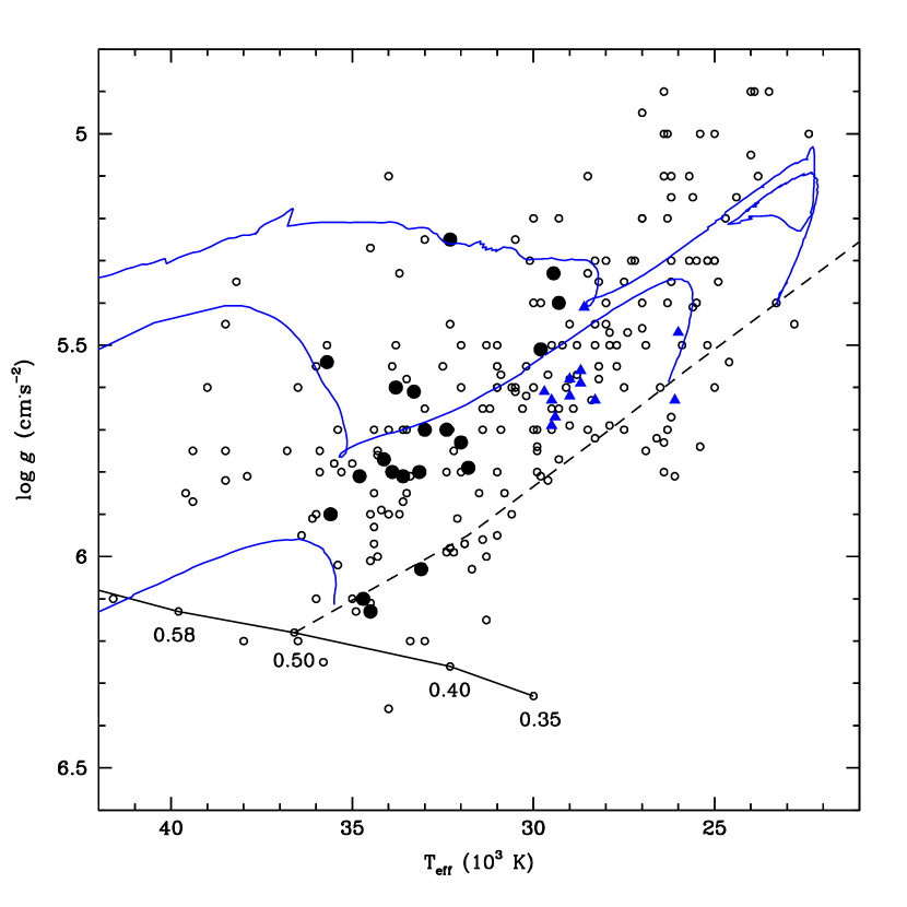
Figure 8: A $\log g-T_{\rm eff}$ diagram showing the location of sdB stars. Filled circles are EC 14026-type pulsators, filled (blue) triangles are PG 1716-type pulsators, and open circles are non-pulsating sdB stars. The dashed line is the zero-age extended horizontal branch, the black line is the zero-age helium main sequence with open circles indicating the total mass. The evolutionary tracks (solid blue lines) were produced using ISUEVOS (Reed et al., 2004).

Figures 9 and 10 show schematic representations of the temporal spectra of all 23 stars, ordered by $\log g$, with the three stars without spectroscopically constrained values at the end. The dotted arrows (blue in the electronic version) indicate frequencies which are only observed occasionally. PG 0014 has dashed arrows (green in the electronic version), indicating frequencies that were only observed using ULTRACAM. To make low-amplitude frequencies visible in the plots, the vertical axes may begin below zero and are scaled so that the highest amplitude peak touches the top line, except for PG 1605, BA09, PG 1325, and EC 20338. All of the latter have one high-amplitude peak that would make the others too small on the plot. Those frequencies are indicated with arrows which pass beyond the top of the plot, though still not to scale. Note that all panels are plotted at different scales. BA09 shows a mixture of short- (EC 14026-type), and long-period (PG 1716-type) oscillations; only the former are shown.

Table 6: Pulsation properties of EC 14026-type pulsators for which follow-up data has been obtained. References for the spectroscopic measurements are as follows: 1) Oreiro et al. 2004; 2) Koen et al. 1999a; 3) O’Donoghue et al. 1997; 4) Koen et al. 1998b; 5) Østensen et al. 2001a; 6) Østensen et al. 2000b; 7) Billéres et al. 2000; 8) Koen 1998; 9) Brassard et al. 2001; 10) O’Donoghue et al. 1998b; 11) Koen et al. 1999b; 12) Silvotti et al. 2002b; 13) Kilkenney et al. 1998; 14) Koen et al. 1998a; 15) Silvotti et al. 2000; U) Unpublished. Parameters in parentheses are inferred using color and pulsation frequencies. NA indicates information that is not available. BA09 also has longer period (PG 1716-type) pulsations and combination frequencies which are not included in this table.

Star	Total	High	Low	$1/\Delta T$	Limit	Resolved?	$T_{\rm eff}$	$\log g$	Power	Amax	Refs
	(#)	(#)	(#)	($\mu$Hz)	(mma)		(K)	($cm\cdot s^{-2}$)	(mma2)	(mma)
BA09	19	3	16	0.4	0.5	No	29446	5.33	4103.92	57.7	1
EC 05217	8	6	2	0.9	1.3	No	32000	5.73	29.36	3.9	2
EC 14026	3	1	2	NA	NA	Yes	34700	6.10	164	12	3
EC 20338	5	3	2	1.2	0.8	No	(35500)	(5.8)	774.43	26.6	U
Feige 48	8	3	5	0.8	0.1	Yes	29500	5.50	69.73	6.4	4
HS 0039	14	6	8	0.8	0.4	Yes	32400	5.70	60.15	4.4	5
HS 0444	3	2	1	0.4	0.6	Yes	33800	5.60	130.1	4.4	5
HS 1824	1	1	0	0.25	0.48	Yes	33100	6.03	11.56	3.4	5
HS 2149	6	6	6	NA	NA	Yes	35600	5.90	28.67	7.0	6
HS 2151	5	5	0	0.5	0.53	Yes	34500	6.13	30.02	3.8	5
HS 2201	5	2	3	0.01	0.5	Yes	29300	5.40	119.94	10.8	6
KPD 1930	39	31	8	0.5	0.8	No	33300	5.61	74.54	3.6	7
KPD 2109	8	6	2	0.4	0.29	Yes	31800	5.79	97.0	6.4	8
PB 8783	10	6	4	0.8	0.1	No	35700	5.54	16.13	2.1	3
PG 0014	13	8	5	0.9	0.48	Yes	34130	5.77	20.37	3.9	9
PG 0048	30	29	1	0.28	0.8	Yes	(34000)	(5.75)	42.16	2.3	U
PG 0154	6	4	2	1.4	0.76	Yes	(35000)	(5.8)	129.34	9.5	U
PG 1047	18	6	12	0.8	0.2	Yes	33150	5.80	87.0	6.7	10
PG 1219	6	4	2	0.8	0.6	Yes	33600	5.81	108.18	6.6	11
PG 1325	14	6	8	0.5	0.8	Yes	34800	5.81	744.27	27.1	12
PG 1336	27	13	14	1.0	0.25	Yes	33000	5.70	83.75	4.7	13
PG 1605	55	5	50	0.8	0.5	Yes	32300	5.25	1802.1	27.4	14
PG 1618	6	6	0	0.3	0.59	Yes	33900	5.80	18.53	2.2	15

Figure 9: Schematic representation of the temporal spectra of sdBV stars with follow-up data ordered by $\log g$ (from lowest to highest). Blue arrows indicate frequencies that are not regularly detected and green arrows for PG 0014 indicate frequencies only detecting using ULTRACAM. Shown here are the stars with lower gravities.

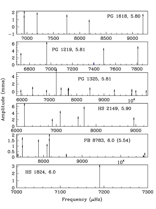
Figure 10: Same as Fig. 9, but for stars with higher gravities. The last three panels are for the stars without a previously determined value of $\log g$.

These two figures show the enormous variety of amplitudes and frequencies detected in sdBV stars. There are only four high-amplitude (here $A>20$ mma) pulsators known and they have a great range (for sdB stars) of gravities and temperatures. There are pulsators with 20+ frequencies that have similar temperatures and gravities to stars with 5 frequencies (e.g., BA09 & HS 2201). If one looks at only the range of gravities from $\log g=5.6$ to 5.7 (about $1\sigma$ in error), there are two stars with more than 20 frequencies yet one star with only three frequencies (but higher amplitudes!).

5.3 Observational tests and trends

In an attempt to bring order to the class as a whole and to find trends in the observational properties, we have organized the data in several ways which have benefited studies of other variable stars. In this subsection we will show the results along with some motivation, but leave in-depth interpretations to the next subsection.

Frequency groupings: Our first arrangement was to put the frequencies shown in Figs. 9 and 10 onto a common frequency scale and make a correction for gravity. Because $p-$mode periods are inversely proportional to the square root of the density, we expect that stars with lower $\log g$ have longer periods (shorter frequencies). This is largely observed in the left panel of Fig. 11. In the right panel, we have rescaled pulsation frequencies by $1/g^{0.75}$ (assuming constant mass) which is an adjustment for both size and density using just $\log g$. For the three sdBV stars without measured gravities, we estimated the gravity from the position of the shortest frequency compared to pulsators with known gravities. These assumed gravities are provided in parentheses in Fig. 11 and Table 6. Such a study of pulsating white dwarfs revealed groups of frequencies which could then be related to individual modes (Clemens, 1994). However, as evidenced by the summation of the right panel, no such groupings occur. The horizontal line just above the summation frequencies (right panel of Fig. 11) shows the effect of an error of $\log g=0.05$ in the rescaling. It is therefore possible that any groups are being smeared out by measurement errors in $\log g$. We attempted to correct for this by fixing the lowest modified frequency to a given value, but no corrections or fixed reference values of $\log g$ show reasonably-separated grouping that could be of use.

Relative pulsation amplitudes: The line lengths in Figs. 9 through 11 indicate another feature that is observed about half the time; one or two amplitudes are significantly higher than the rest. To parameterize this phenomenon, we have denoted frequencies whose amplitudes are within a factor of five of the highest amplitude as “high” amplitudes; the remainder are “low” amplitudes. The numbers that fall into each category, along with the highest amplitude observed ($A_{\rm max}$) for each star, are provided in Table 6. The factor of five was chosen so that all amplitudes greater than 10 mma for PG 1605 and BA09 would fall into the high category. Additionally, we use the published (typically average) amplitudes, even though some vary by large amounts (discussed below).

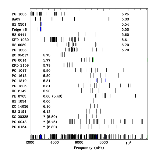
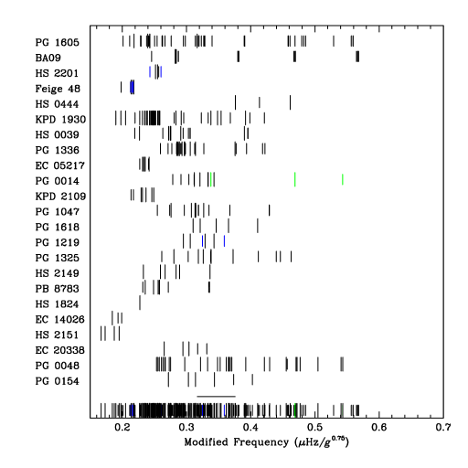
Figure 11: Schematic representations of pulsation frequencies organized by $\log g$. The lines used to indicate frequencies have two lengths, with the shorter lengths indicating frequencies with amplitudes a factor of 5 smaller than the highest amplitude. The right panel has a frequency correction for $\log g$ and both panels include a summation of all frequencies at the bottom.

Figure 12: Comparison of number of “high” amplitude frequencies (H) to the total number of frequencies (T). Double sized points indicate two stars with the same quantities. The right panel compares this ratio with the surface gravity.

The left panel of Fig. 12 shows the ratio of high (H) to total (T) number of frequencies against the total number of frequencies; the values of which are also provided in Table 6. One might suspect that if a star has one high amplitude, all amplitudes are relatively higher and thus easier to detect. This appears not to be the case, since the points make a scatter diagram. In the right panel of Fig. 12, we show the H/T ratio against $\log g$. It might be expected that gravity plays a factor, in that it is easier to pulsate radially at lower gravities. The values of H/T are indeed positively correlated with gravity, but the correlation coefficient is only 0.59.

A more quantitative approach is shown in Fig. 13, where we analyse the distribution of amplitudes and power in each star. For each star, the frequencies were sorted by increasing amplitude and the cumulative distribution of amplitudes (or power) was computed at intervals of 10% of the total. This process is shown in Fig. 14 for the star HS 0039. The 14 frequencies from Table 3 are shown as squares with their amplitudes given by the right-hand Y-axis. The circles indicate the cumulative fractional amplitude for each frequency, connected by the solid line, with their scale given by the left-hand Y-axis. The points for HS 0039 in the left panel of Fig. 13 correspond to the locations in Fig. 14 where the dotted lines intersect the solid line. The top solid line in Fig. 13 connects the points for the 90^th percentile, the next line for the 80^th percentile, and so on. The left panel of Fig. 13 displays these points, or amplitude distribution, for the 20 stars with more than five frequencies. Their designations are provided along the bottom in order of increasing gravity. Low values indicate that the top one or two amplitudes contain a large fraction of the total amplitude (Fig. 14 would show a sharply peaked line). The right panel displays the distribution of power which we define as the sum of the squares of the amplitudes; the power and the maximum amplitude $A_{\rm max}$ are provided in Table 6. On average, the lowest-amplitude half of the frequencies contribute about 25% of the total amplitude and 9.6% of the total power.

If the amplitudes or power were evenly distributed (equal-height amplitudes) then $f_{i}/f_{T}$ would equal $A_{i}/A_{T}$ (or $\sqrt{P_{i}/P_{T}}$). The corresponding distribution in Fig. 14 would be a straight diagonal line. There is a trend in Fig. 13 in that the contours are closest at low gravities and most diffuse at high gravities. However, these trends are dominated by four stars (two at each end) and are not representative of the majority of the class. In the middle of each panel, there is a large dispersion in values, with neighbouring stars transmitting most of their power through one frequency, or distributing it more equally.

In each panel, the dashed line indicates the fractional amplitude or power emitted by the frequency with the highest amplitude. For PG 1325, the one highest amplitude has 99% of the total, while for PG 0048 it is only $\sim 12$%. The dashed line in Fig. 14 indicates that for HS 0039, the highest amplitude frequency has 20% of the combined amplitudes. While it is difficult to assign significance to this plot as the number of pulsators is still relatively low, it is suggestive that in lower gravity stars the pulsation energy is channeled into relatively few (or one) frequencies even though many frequencies are available.

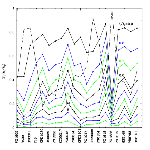
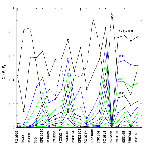
Figure 13: Distribution of amplitudes (left panel) and power (right panel) for pulsators with at least five frequencies. The stellar designations are provided at the bottom and are organized by increasing gravity similar. Each colored line indicates a decreasing fraction of pulsation frequencies (from top to bottom), with the first four lines labeled. The dashed line indicates the fractional amplitude or power of the highest amplitude frequency in each star.

Figure 14: Distribution of amplitudes for HS 0039. The frequencies are organized from lowest to highest amplitude with the amplitudes indicated by filled squares (on the scale of the right-hand axis). The cumulative fractional amplitudes are indicated by filled circles and connected by a solid line. The vertical dotted lines are locate at 10% intervals to indicate the points in Fig. 13 and the horizontal dashed line (on the scale of the left-hand axis) indicates the fractional amplitude of the highest amplitude frequency.

Multiplet structure: As the prototype for multiplet structure in pulsating white dwarfs, PG 1159 showed that observational determination of the modes can lead to tight constraints on the models (Winget et al., 1991). With detailed studies of 23 pulsating sdBV stars, it would be hoped that a similar star of this class would have been detected. However, this has not been the case: multiplet structure has been conspicuously absent, even from rich pulsators. The only confirmed case of multiplets caused by rotational splitting is Feige 48 (Reed et al., 2004; O’Toole et al., 2004), while another likely candidate is BA09 (Baran et al., 2005). There are also marginal cases for rotationally induced multiplet structure in HS 2201, PB 8783, PG 0014, PG 1047, and PG 1605 none of which have been confirmed by additional observations. KPD 1930 and PG 1336 are both known to be in short period binaries and frequency splittings are commensurate with the binary period. An initial interpretation did not attribute these to rotational splitting, but rather to tidal effects induced by the companion (Reed et al., 2006c, d).

A possible reason for the lack of observed multiplet structure was proposed by Kawaler & Hostler (2005). Their picture invokes sharp differential rotation in rapidly spinning cores to modify the frequency spacings. Exceptions would be for those stars in close binaries where rotations are tidally locked.

Another multiplet pattern that has emerged lately is the “Kawaler-scheme” (Kawaler et al. 2006) a purely mathematical formalism based on an asymptotic-like relationship for the frequencies: $f(i,j)=f_{o}+i\times\delta+j\times\Delta$ where $i$ has integer values, $j$ is limited to values of $-1,\,0,$ and $1$, $\delta$ is usually a small spacing and $\Delta$ is usually a large spacing. Their Table 3 indicates the significance of their predicted frequencies to those observed in several stars. However, it is also known that the Kawaler-scheme does not fit several pulsators (including HS 0039) and so we merely make note of the scheme but await a full report in a forthcoming paper.

Frequency density: As discussed in §4.2, another tool at our disposal is the mode density. Although the mode density does not help to assign modes to individual frequencies, we can set limits on the number of degrees ($\ell$) per order ($n$) required to create the observed frequency density from currently available models of Charpinet et al. (2001, hereafter CFB01) and of Reed et al. (2004).

Figure 15 shows the mode density, plotted against $\log g$, with the dotted line indicating 3 frequencies per 1000 $\mu$Hz (all $\ell\leq 2,m=0$ modes) and the dashed line indicating 9 frequencies per 1000 $\mu$Hz (all possible $2\ell+1$ $m$ modes). Starred points indicate those pulsators for which we have inferred the $\log g$ values. Less than 20% of sdBV stars have mode densities below 3 per 1000 $\mu$Hz, while more than 25% have mode densities too high to be reconciled with $\ell\leq 2$ modes even if all possible $m$ values are used. It therefore seems reasonable to conclude that $\ell\geq 3$ modes must be excited.

Figure 15: Mode density of pulsators organized by gravity. The dotted line indicates the limit of 3 frequencies per 1000 $\mu$Hz (all $m=0$ frequencies) and the dashed line indicates the limit of 9 frequencies per 1000 $\mu$Hz (all possible $2\ell+1$ $m$ values) assuming $\ell\leq 2$.

Amplitude variability: A criterion outlined in Christensen-Dalsgaard et al (2001; hereafter JCD01) and previously applied to several sdBV stars (Pereira & Lopes 2005; Zhou et al. 2006; Reed et al. 2006a, 2007) is to compare the average amplitude $\langle A\rangle$ to the standard deviation of the amplitudes, $\sigma(A)$. For stochastically excited pulsations, this ratio should have a value near 0.5. For all resolvable frequencies in our target stars, we have calculated both parameters and their ratios which are given in columns 3 to 5 of Table 7 and plotted in Fig. 16. Columns 6 and 7 of Table 7 list the maximum and minimum observed amplitudes and column 8 gives the maximum time-scale over which the observations are sensitive to amplitude variations. In the Figure, triangles (squares) indicate frequencies known to have stable (not-stable) phases, circles indicate frequencies with ambiguous or no phase information and stars indicate the PG 0048 frequencies, which are known to have stochastic-like properties (Reed et al. 2007). Stochastic oscillations do not have stable pulsation phases and so frequencies with stable phases should be driven rather than stochastically excited. Amplitudes for HS 2201 came from Silvotti et al. (2002a) and no errors were published, so no errorbars appear in the Figure.

Just like their average amplitudes and frequency density, the only conclusion we can draw from Fig. 16 and Table 7 is sdBV stars show a large variety of amplitude variations. Of course it is known that many classes of pulsators show large amplitude differences and that correlations between excitation rates and amplitudes are weak at best, but these results indicate that there is no clear separation in amplitude variability for phase-stable and unstable frequencies. As such, it follows that the JCD01 criterion is likely not applicable for these stars. One last note is that our calculations do not include frequencies that have been observed only one time (as in PG 1219 and Feige 48) or stars for which we do not have the data. Both EC 14026 and EC 20338 are reported to have sufficient amplitude variability that frequencies completely disappear between observing seasons (Kilkenny et al. 2006b).

Table 7: Mean amplitude, standard deviation, and their ratio for readily resolvable frequencies. Columns 6 through 8 provide the maximum and minimum measured amplitudes and the longest time covered by the observations. Except for HS 2201, all amplitudes and standard deviations have been calculated specifically for this paper from data we have. HS 2201 amplitudes are directly from Silvotti et al. 2002a and no error estimates were provided. Note that all frequencies are in $\mu$Hz and all amplitudes are in mma.

Star	Frequency	$\langle A\rangle$	$\sigma(A)$	$\sigma(A)/\langle A\rangle$	$A_{max}$	$A_{min}$	Timescale
BA09	2807	45.76	1.36	$0.03\pm 0.004$	52.89	44.30	53 days
	2823	10.30	2.15	$0.21\pm 0.03$	20.68	8.20	53 days
	2824	14.19	0.68	$0.05\pm 0.02$	15.2	11.50	53 days
	2827	3.60	0.24	$0.07\pm 0.03$	4.86	2.4	53 days
	3776	1.58	0.57	$0.36\pm 0.06$	4.35	1.4	53 days
	3791	1.26	0.50	$0.39\pm 0.07$	2.39	0.14	53 days
EC 05217	4595	3.04	0.79	$0.26\pm 0.10$	4.59	2.74	9 days
	4629	4.32	0.73	$0.17\pm 0.06$	5.16	3.05	9 days
Feige 48	2851	3.83	2.85	$0.74\pm 0.20$	9.46	1.31	8 years
	2877	5.80	2.14	$0.37\pm 0.08$	10.4	1.89	8 years
	2906	4.10	1.44	$0.35\pm 0.08$	5.28	0.58	8 years
HS 0039	4271	4.45	0.17	$0.04\pm 0.03$	5.03	3.82	30 days
	5482	2.35	1.30	$0.56\pm 0.17$	4.44	0.12	30 days
	7348	1.09	0.77	$0.70\pm 0.24$	3.17	0.37	30 days
HS 0444	5903	2.59	0.44	$0.17\pm 0.01$	3.16	1.76	30 days
	7312	11.04	0.61	$0.06\pm 0.02$	12.39	10.11	30 days
HS 1824	7190	3.01	0.92	$0.30\pm 0.06$	5.26	0.87	47 days
HS 2151	6616	3.89	0.47	$0.12\pm 0.05$	5.14	3.36	23 days
	6859	1.73	0.42	$0.24\pm 0.10$	2.45	1.31	23 days
	7424	1.19	0.22	$0.18\pm 0.12$	1.66	0.95	23 days
HS 2201	2738	0.39$\dagger$	0.08	0.20	0.48	0.34	1 year
	2824	4.85$\dagger$	0.54	0.13	5.65	4.23	1 year
	2861	10.31$\dagger$	0.54	0.05	10.88	9.77	1 year
	2881	1.16$\dagger$	0.16	0.13	1.34	1.00	1 year
	2922	0.6$\dagger$	0.04	0.07	0.64	0.56	1 year
KPD 2109	5045	2.64	1.05	$0.40\pm 0.11$	4.80	0.59	32 days
	5093	6.45	0.75	$0.12\pm 0.10$	8.09	5.21	32 days
	5212	1.65	0.54	$0.32\pm 0.09$	3.14	0.31	32 days
	5481	6.21	0.45	$0.07\pm 0.10$	7.41	4.96	32 days
PB 8783	7870	1.68	0.27	$0.16\pm 0.09$	2.4	1.4	14 days
	8092	1.19	0.24	$0.20\pm 0.11$	1.6	0.5	14 days
PG 0048	5245	1.74	0.58	$0.33\pm 0.09$	2.44	0.93	15 days
	7237	1.45	0.40	$0.25\pm 0.10$	2.13	0.27	15 days
PG 0154	6090	9.57	0.21	$0.02\pm 0.03$	10.28	8.97	8 days
	6785	3.75	1.16	$0.31\pm 0.11$	5.31	1.50	8 days
	7032	3.57	0.83	$0.23\pm 0.09$	5.05	1.33	8 days
	7688	2.61	0.28	$0.11\pm 0.20$	3.28	0.84	8 days
	8362	1.12	0.22	$0.19\pm 0.16$	1.86	0.13	8 days
	9015	1.03	0.21	$0.21\pm 0.16$	2.53	0.51	8 days
PG 1219	6722	3.35	0.49	$0.15\pm 0.03$	4.72	2.15	4 years
	6961	7.00	0.46	$0.07\pm 0.01$	8.06	5.73	4 years
	7490	5.19	1.74	$0.33\pm 0.07$	8.48	2.94	4 years
	7808	6.35	1.65	$0.26\pm 0.05$	9.85	4.44	4 years
PG 1325	7253	23.21	2.12	$0.09\pm 0.03$	26.04	18.58	14 days

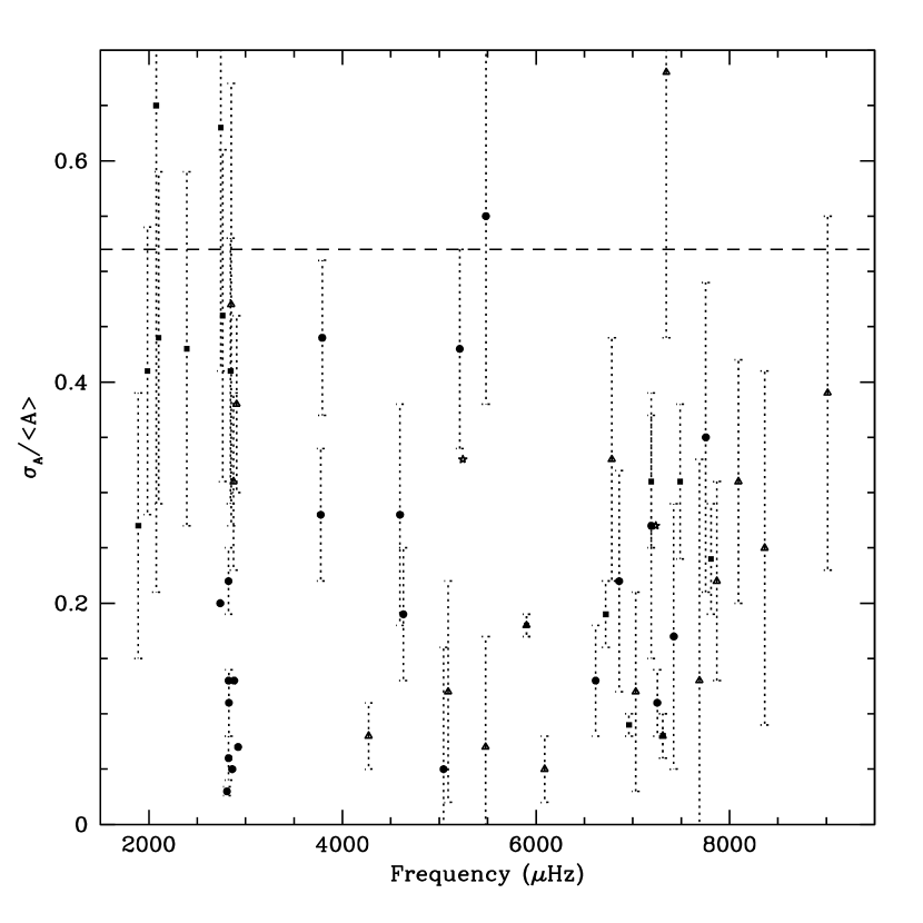
Figure 16: $\sigma(A)/\langle A\rangle$ of individual frequencies. Triangles (squares) indicate phase-stable (-not-stable) frequencies, circles indicate frequencies with no phase information or indeterminate phase stability and stars indicate the PG 0048 frequencies which appear stochastic in nature. The dashed line is the JCD01 stochastic value.

Table 8: Table 7 continued

Star	Frequency	$\langle A\rangle$	$\sigma(A)$	$\sigma(A)/\langle A\rangle$	$A_{max}$	$A_{min}$	Timescale
PG 1605	1891	9.6683	3.38	$0.35\pm 0.12$	16.30	7.80	7 years
	1986	12.06	4.62	$0.38\pm 13$	14.77	2.0	7 years
	2076	24.51	23.74	$0.97\pm 0.44$	56.92	8.4	7 years
	2102	29.24	12.32	$0.42\pm 0.15$	48.9	13.4	7 years
	2392	3.52	1.54	$0.44\pm 0.16$	6.65	2.2	7 years
	2743	14.61	8.48	$0.58\pm 0.22$	29.0	5.02	7 years
	2763	6.80	2.88	$0.42\pm 0.15$	10.89	2.5	7 years
	2845	4.87	1.71	$0.35\pm 0.12$	7.1	2.0	7 years
PG 1618B	7191	2.13	0.44	$0.21\pm 0.12$	3.6	1.14	45 days
	7755	1.75	0.50	$0.28\pm 0.14$	3.50	0.76	45 days

Comparison with theoretical instability contours: We can make a direct comparison between the instability zone of the second-generation pulsation models of Charpinet et al. (2001) and observed pulsation properties. Figures 17 and 18 are used for these discussions. In all the plots, filled circles are the sdBV stars of this study (stars indicate EC 20338, PG 0048, and PG 0154), open circles are sdB stars (and inferred to be non-pulsators) from the Hamburg-Schmidt survey (Edelmann et al., 2003), Moehler et al (1990), and Saffer et al. (1994), and filled (blue) triangles are PG 1716-type pulsators (Green et al. 2003). The contours are reproduced from CFB01 with the outside contour representing one unstable $\ell=0$ frequency with each interior contour representing an additional unstable $\ell=0$ frequency up to $N=7$.

In the left panel of Fig. 17, we determine how discriminating the instability zone is by examining the ratio of pulsators to non-pulsators within each contour. However, we need to have an exception for the red (cool) edge of the instability zone. There is an indication that sdB stars may switch from EC 14026- to PG 1716-type pulsators in this region. As such, this region (separated with a dotted line) should be excluded; particularly since it is stated that “all cool sdB stars of low gravity may be PG 1716 pulsators” (Fontaine et al. 2006). Working from the inside ($N=7$) contour outward, the fraction of pulsating to non-pulsating sdB stars is: $N\geq 7$, 50%; $N\geq 6$, 25%; $N\geq 5$, 25%; $N\geq 4$, 22%; $N\geq 3$, 21%; $N\geq 2$, 20%; $N\geq 1$, 20% and the fraction of all sdB stars within the contours is $N\geq 7$, 12%; $N\geq 6$, 52%; $N\geq 5$, 80%, $N\geq 4$, 90%; $N\geq 3$, 92%; $N\geq 2$, 95%; $N\geq 1$, 95%; $N<1$, 100%. There does appear to be a relationship between the interior instability ($N=7$) contour and fraction of pulsators. Yet outside of the first contour, the ratio only changes by 5% and all of the EC 14026-type pulsators are within the first three contours. Yet so are 80% of all sdB stars. So while the contours match where the pulsators are, they also match where most sdB stars with $T_{\rm eff}\geq$30 000 K are.

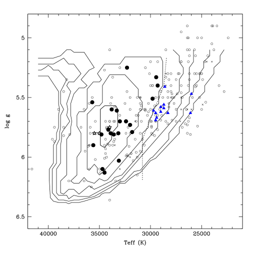
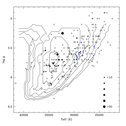
Figure 17: Comparison of observed sdB stars to pulsational instability contours (adapted from CFB01). Open circles are non-pulsating sdB stars, filled circles are EC 14026-type pulsators, and (blue) triangles are PG 1716-type pulsators. Left panel includes a dashed line indicating the inferred separation between EC 14026 and PG 1716-type pulsators and in the right panel the dot size corresponds to the number of total pulsation frequencies detected.

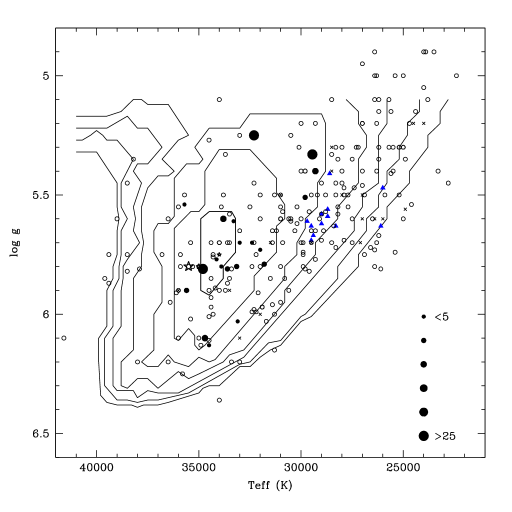
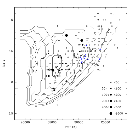
Figure 18: Same as in Fig. 17 except that dot sizes for pulsators represent $A_{max}$ (left panel) and total pulsation power (right panel).

The remaining panels of Figs. 17 and 18 show the same points, but the size of the dots correlate with the following observed properties; the number of pulsation frequencies (right panel of Fig. 17), the maximum amplitude ($A_{max}$), and total pulsation power. $A_{max}$ and total pulsation power are related as power is dominated by a few high-amplitude frequencies. Stars such as PG 0048 with many, but low amplitude frequencies cannot match the power of a single $A\geq 20$ mma frequency. We would expect a correlation of the instability contours with the number of frequencies detected, as each interior contour increases the number of theoretically unstable frequencies, but such is not the case. From §5.2, we know that it is not a detection issue as rich pulsators occur with both low and high amplitudes. In fact there seems to be no correlation whatsoever with the largest points (largest number of frequencies, highest amplitude and most pulsation power) occupying multiple regions of the $\log g-T_{\rm eff}$ diagrams and similar results for the smallest points. As such the group properties do not add observational support to the driving theory.

6 Conclusions

From extensive follow-up data acquired at MDM observatory, we are confident that we have resolved the pulsation spectra of two additional pulsating sdB stars. For HS 0039, we detect 10 additional frequencies bringing the total to 14 and for HS 0444, we confirm the two frequencies of the discovery data and detect an additional low amplitude frequency. We have also noted that while the amplitudes and phases of HS 0444 appear very steady over the duration of our observations, those in HS 0039 did not, but rather have varied considerably. This is illustrative of the variety observed in sdBV stars where some stars can have very simple and/or stable pulsation spectra while others can be quite rich, with tens of frequencies that may change amplitudes on short time scales.

Since the discovery of sdBV stars in 1996, more than 23 of the 34 known EC 14026-type pulsators have received follow-up observations. We have examined these 23 stars for which extended timebase (and often multisite) observations have been acquired. We have searched for trends in frequency groupings, the number of high (H) amplitude to total (T) frequencies, and frequency density as a function of gravity and note that the only trend seems to be a weak relationship between the H/T ratio and gravity: The lowest gravity pulsators have the smallest H/T ratio (a few very high amplitude frequencies) while the highest gravity pulsators have H/T$\approx 1$ (relatively even amplitudes distributed amongst the observed frequencies).

We examined amplitude stability, which has been used to infer stochastically excited oscillations in other variable classes and previously applied to sdB pulsators. And while many pulsation frequencies fit the JCD01 value, the distribution between those and amplitude-stable and presumably driven is relatively smooth with no clear separations. However, phase-stable frequencies, some with quite large variability, preclude them from being stochastically excited and so the simplest conclusion is that the JCD01 criteria is not appropriate for sdBV stars.

We compared pulsators to theoretical instability contours to search for relationships that correlate with current driving theory. While there is a weak concentration of pulsators precisely where expected, these same contours include more than 80% of all sdB stars in our sample with $T_{\rm eff}\geq 30\,000$ K (an inferred cut-off for PG 1716-type pulsators) and there is no correlation between the contours and the number of pulsation frequencies, nor their maximum amplitude or total pulsation power. It would be nice if we could note that any correlation is canceled by stars with lower gravities requiring less energy to drive higher amplitudes which results in more frequencies being detected, but this is also not the case as the amplitudes of neighboring stars anywhere in the $\log g-T_{\rm eff}$ plane can have amplitudes that differ by more than an order of magnitude.

In the end, what we have uncovered in our examination of sdBV stars is the large variety they encompass. Subdwarf B pulsators seem to exist at all temperatures and gravities (though we only examined the EC 14026-type pulsators at $T_{\rm eff}\geq 30\,000$ K) that sdB stars do and at roughly the same concentrations. Regardless of temperature or gravity (and thus evolutionary age and/or total mass and/or envelope mass and/or metallicity) pulsators can have relatively high ($\geq 20$ mma) or low ($\leq 2$ mma), stable or unstable amplitudes and the frequency density can be quite high or very low. We hope that our investigation of these 23 well-studied sdBV stars will be useful and bring new insight to their theoretical perspectives. Additionally, we also hope that this study will be useful for observers pursuing multicolour photometry and time-series spectroscopy. We anticipate that such works will be required for an overall understanding of sdB pulsations, yet these more detailed observations require that the pulsation characteristics of the star be known beforehand. So even though 23 of 34 known sdBV stars have received follow-up observations, there is still a long way to go both observationally and theoretically.

ACKNOWLEDGMENTS: We would like to thank the MDM and McDonald observatory TACs for generous time allocations, without which this work would not have been possible. We would also like to thank Dave Mills for his help with the Linux camera drivers, Darragh O’Donoghue, Chris Koen, Dave Kilkenny and Andrzej Baran for kindly sharing their data. We also thank the many observers who have provided support for our campaigns, particularly those at Lulin and Suhora observatories who have helped on many campaigns. Support for DMT came in part from funds provided by the Ohio State University Department of Astronomy. This material is based in part upon work supported by the National Science Foundation under Grant Number AST007480. Any opinions, findings, and conclusions or recommendations expressed in this material are those of the author(s) and do not necessarily reflect the views of the National Science Foundation.

References

- Baran et al. (2005) Baran A., Pigulski A., Koziel D., Ogloza W., Silvotti R., Zola S., 2005, MNRAS, 360, 737
- Billr̀es et al. (2000) Billères M., Fontaine G., Brassard P., Charpinet S., Liebert J., Saffer R.A., 2000, ApJ, 530, 441
- Brassard et al. (2001) Brassard P., Fontaine G., Billères M., Charpinet S., Liebert J., Saffer R. A., 2001, ApJ, 563, 1013
- Charpinet et al. (2001) Charpinet S., Fontaine G., Brassard P., 2001, PASP, 113, 775
- Charpinet et al. (2002) Charpinet S., Fontaine G., Brassard P., Dorman, B., 2002, ApJS, 140, 469
- Charpinet et al. (2005) Charpinet S., Fontaine G., Brassard P., Green E.M., Chayer P., 2005, A&A, 437, 575
- Christensen et al. (2001) Christensen-Dalsgaard J., Kjeldsen H., Mattei J.A., 2001, ApJ, 562, L141
- Clemens (1994) Clemens J.C., 1994, PASP, 106, 1322
- Daszyńska-Daszkiewicz et al. (2005) Daszyńska-Daszkiewicz J., Dziembowski W. A., Pamyatnykh A. A., Breger M., Zima W., Houdek, G., 2005, A&A, 438, 653
- Edelmann et al. (2003) Edelmann H., Heber U., Hagen H.-J., Lemke M., Dreizler S., Napiwotzki R., Engels D., 2003, A&A, 400, 939
- Fontaine et al. (2006) Fontaine G., Green E. M., Chayer P., Brassard P., Charpinet S., Randall, S.K., 2006, BaltA, 15, 211
- Green et al. (2003) Green E. M., et al., 2003, ApJ, 583, L31
- Harms et al. (2006) Harms S.L., Reed M.D., O’Toole S.J., 2006, BaltA, 15, 251
- Heber (1984) Heber U., 1984, A&A, 130, 119
- Heber, Reid, Werner (1999) Heber U., Reid I.N., Werner K., 1999, A&A, 348, 25
- Heber, Reid, Werner (2000) Heber U., Reid I.N., Werner K., 2000, A&A, 363, 198
- Jeffery et al. (2004) Jeffery C.S., Dhillon V.S., Marsh T.R., Ramachandran B., 2004, MNRAS, 352, 699
- Kawaler & Hostler (2005) Kawaler S.D., Hostler S.R., 2005, ApJ, 621, 432
- Kawaler et al. (2006) Kawaler S.D., Vuc̆ković M., The WET Collaboration, 2006, BaltA, 15, 283
- Kilkenny et al. (1997) Kilkenny D., Koen C., O’Donoghue D., Stobie R.S., 1997, MNRAS, 285, 640
- Kilkenny et al. (1998) Kilkenny D., O’Donoghue D., Koen C., Lynas-Gray A. E., van Wyk F., 1998, MNRAS, 296, 329
- Kilkenny et al. (1999) Kilkenny D., et al., 1999, MNRAS, 303, 525
- Kilkenny et al. (2002) Kilkenny D., et al., 2002, MNRAS, 331, 399
- Kilkenny et al. (2003) Kilkenny D., et al. (The Whole Earth Telescope collaboration) 2003, MNRAS, 345, 834
- Kilkenny et al. (2006a) Kilkenny D., Kotze J.P., Jurua E., Brownstone M., Babiker H.A. 2006a, BaltA, 15, 255
- Kilkenny et al. (2006b) Kilkenny D., Stobie R.S., O’Donoghue D., Koen C., Hambly N., MacGillivray H., Lynas-Gray, A.E., 2006b, MNRAS, 367, 1603
- Koen (1998) Koen C., 1998, MNRAS, 300, 567
- Koen et al. (1998a) Koen C., O’Donoghue D., Kilkenny D., Lynas-Gray A. E., Marang F., van Wyk F., 1998a, MNRAS, 297, 317
- Koen et al. (1998b) Koen C., O’Donoghue D., Pollacco D. L., Nitta A., 1998b, MNRAS, 300, 1105
- Koen et al. (1999a) Koen C., O’Donoghue D., Kilkenny D., Stobie R. S., Saffer R. A., 1999a, MNRAS, 306, 213
- Koen et al. (1999b) Koen C., O’Donoghue D., Pollacco D. L., Charpinet, S., 1999b, MNRAS, 305, 28
- Moehler et al. (1990) Moehler S., de Boer K. S., Heber, U., 1990, A&A, 239, 265
- O’Donoghue et al. (1997) O’Donoghue D., Lynas-Gray A.E., Kilkenny D., Stobie R.S., Koen C., 1997, MNRAS, 285, 657
- O’Donoghue et al. (1998a) O’Donoghue D., et al., 1998a, MNRAS, 296, 296
- O’Donoghue et al. (1998b) O’Donoghue D., Koen C., Lynas-Gray A. E., Kilkenny D., van Wyk F., 1998b, MNRAS, 296, 306
- Oreiro et al. (2004) Oreiro R., Ulla A., Pérez H.F., Østensen R., Rodríguez L.C., MacDonald J., 2004, A&A, 418, 243
- Østensen et al. (2001) Østensen R., Heber U., Silvotti R., Solheim J.-E., Dreizler S., Edelmann H., 2001a, A&A, 378, 466
- Østensen et al. (2001b) Østensen R., Solheim J.E., Heber U., Silvotti R., Dreizler S., Edelmann H., 2001b, A&A, 368, 175
- O’Toole et al. (2004) O’Toole S.J., Heber U., Benjamin R.A., 2004, A&A, 422, 1053
- Pereira & Lopes (1005) Pereira T.M.D., Lopes, I.P., 2005, ApJ, 622, 1068
- Reed et al. (2004) Reed M.D., et al., (The Whole Earth Telescope Collaboration), 2004, MNRAS, 348, 1164
- Reed et al. (2005) Reed M.D., Brondel B.J., Kawaler S.D., 2005, ApJ, 634, 602
- Reed et al. (2006a) Reed M.D., Eggen J.R., Zhou A.-Y., Terndrup D.M., Harms S.L., An D., Hashier M.A., 2006a MNRAS, 369, 1529
- Reed et al. (2006b) Reed M.D., et al., 2006b, MmSAI, 77, 476
- Reed et al. (2006c) Reed M.D., Whole Earth Telescope Xcov 21 and Xcov 23 collaborations, 2006c, BaltA, 15, 269
- Reed et al. (2006d) Reed M.D., Whole Earth Telescope Xcov 21 and Xcov 23 collaborations, 2006d, MmSAI, 77, 417
- Reed et al. (2007) Reed M.D., et al., 2007, ApJ, in press.
- Saffer et al. (1994) Saffer R.A., Bergeron P., Koester D., Liebert J., 1994, ApJ, 432, 351
- Silvotti et al. (2000) Silvotti R., Solheim J.-E., Gonzalez Perez J. M., Heber U., Dreizler S., Edelmann H., Østensen R., Kotak R., 2000, A&A, 359, 1068
- Silvotti et al. (2002a) Silvotti R., et al., 2002a, A&A, 389, 180
- Silvotti et al. (2002b) Silvotti R., Østensen R., Heber U., Solheim J.-E., Dreizler S., Altmann M., 2002b, A&A, 383, 239
- Silvotti et al. (2006) Silvotti R., et al., 2006, A&A, 459, 557
- Vuc̆ković et al. (2006) Vuc̆ković M., et al. (The Whole Earth Telescope Collaboration), 2006, ApJ, 646, 1230
- Winget et al. (1991) Winget D.E., et al. (The Whole Earth Telescope Collaboration), 1991, ApJ, 378, 326
- Zhou et al. (2006) Zhou A.-Y., et al., 2006, MNRAS, 367, 179