Large radius exciton in single-walled carbon nanotubes

Abstract

The spectrum of large radius exciton in an individual semiconducting single-walled carbon nanotube (SWCNT) is described within the framework of elementary potential model, in which exciton is modeled as bound state of two oppositely charged quasi-particles confined on the tube surface. Due to the parity of the interaction potential the exciton states split into the odd and even series. It is shown that for the bare and screened Coulomb electron-hole ($e$-$h$) potentials the binding energy of even excitons in the ground state well exceeds the energy gap. The factors preventing the collapse of single-electron states in isolated semiconducting SWCNTs are discussed.

PACS number(s): 78.67.Ch

1 Introduction

Many experimental papers on the optical absorption in SWCNTs describe obtained results in terms of band-to-band direct transitions between single particle states, though it is clear that the inherent to 1D systems strong interparticle interaction cannot be neglected. It seems obvious that the strong electron-hole attraction should bind electron-hole pairs in SWCNTs into Wannier-Mott like excitons. Moreover, the exciton contributions were already revealed experimentally in optical absorption spectra [1], [2], and in spectra of fluorescence [3]-[5] of individual SWCNTs, as well the exciton properties were studied by the Raman spectroscopy [6]. There are also some works devoted to the theoretical study of excitons in CNTs [7]-[12]. However, as it follows from results of the latter a simple translation of basic hydrogen-like models of 3D large radius excitons fails to function in one dimension without a certain specification. Remind that once the centrum of mass has been removed and the screening effect from the tube charges is ignored the 1D model exciton Hamiltonian may be formally given by the expression

$$\widehat{H}=-\frac{\hbar^{2}}{2\mu}\frac{\mathrm{d}^{2}}{\mathrm{d}z^{2}}-\frac{e^{2}}{\varepsilon}\frac{1}{|z|},$$ (1.1)

where $\mu$ is the exciton reduced effective mass and $\varepsilon$ is the dielectric constant of medium surrounding the tube. The functions $\phi(z)$ from the domain of differential expression (1.1) in $\mathbf{L}_{2}(-\infty,\infty)$ are twice differentiable on the semi-axis $(-\infty,0)$, $(0,\infty)$, and belong together with their derivatives for each $\delta>0$ to the subspaces $\mathbf{L}_{2}(-\infty,-\delta)$, $\mathbf{L}_{2}(\delta,\infty)$, and also satisfy a certain boundary conditions at the point $z=0$, which provide the self-adjointness of $\widehat{H}$. If there are no reasons for breaking of the tube reflection symmetry or, in other words, of the action and reaction law, then only those self-adjoint extensions of the above differential operator are physically admissible, for which the subspaces of even and odd functions from $\mathbf{L}_{2}(-\infty,\infty)$ are invariant with respect to $\widehat{H}$.

For less singular than the bare Coulomb even potentials $V(z)=V(|z|)$, for example, for potentials satisfying the condition

$$\int\limits_{0}^{L}|V(z)|^{2}\mathrm{d}z<\infty,\qquad 0<L<\infty,$$

the corresponding Hamiltonians $\widehat{H}$ could be represented as the sum of the standardly defined self-adjoint operator of kinetic energy and the subordinated operator of potential energy that is the multiplication operator by $V(z)$. In such cases the functions from the domains $\mathcal{D}(\widehat{H})$ of $\widehat{H}$ are continuous and have continuous first derivative at $z=0$, and the corresponding odd and even functions from $\mathcal{D}(\widehat{H})$ should satisfy the natural boundary conditions $\phi(0)=0$ and $\phi^{\prime}(0)=0$, respectively. The spectra of bound states are then the set of negative eigenvalues of the boundary problem for the differential equation

$$-\frac{\hbar^{2}}{2\mu}\frac{\mathrm{d}^{2}}{\mathrm{d}z^{2}}\phi(z)-V(z)\phi(z)=E\phi(z)$$

on the semi-axis $(0,\infty)$ with the boundary conditions $\phi(0)=0$ for the odd series and $\phi^{\prime}(0)=0$ for the even series, respectively.

For the Coulomb potential in one dimension the operator of potential energy is not subordinated to that of kinetic energy and the Hamiltonian $\widehat{H}$ cannot be simply represented as their sum, and hence the Hamiltonian in this case becomes indeterminate. Among self-adjoint extensions of the differential operator (1.1) there are infinitely many of those for which subspaces of odd and even functions are invariant. These extensions differ in self-adjoint boundary conditions at $z=0$ and, accordingly, they can be distinguished by energies of their ground states. Since functions from the domain of any such extension are non-differentiable at $z=0$, it is impossible without additional physical considerations to single out the unique ”correct” among suitable self-adjoint boundary conditions at $z=0$.

For the bare Coulomb potential one of possible extensions compatible with $z$-inversion symmetry is the decaying extension $\widehat{H}_{0}$ defined by the boundary condition: $\phi(0)=0$, that is for any $\phi$ from the domain of $\widehat{H}_{0}$ we have

$$\left\{\begin{array}[]{c}\left(\widehat{H}_{0}\phi\right)(z)=-(\hbar^{2}/2\mu)\phi^{\prime\prime}(z)+(e^{2}/\varepsilon z)\phi(z),\ z<0;\\ \\ \left(\widehat{H}_{0}\phi\right)(z)=-(\hbar^{2}/2\mu)\phi^{\prime\prime}(z)-(e^{2}/\varepsilon z)\phi(z),\ z>0;\\ \\ \phi(-0)=\phi(+0)=0.\end{array}\right.$$ (1.2)

This Hamiltonian was obtained in [13], [14] as a result of formal passage to the limit for some sequences of 1D Hamiltonians with regularized at $z=0$ Coulomb potentials. Note, that not only subspaces of odd and even functions, but also the subspaces of functions with supports on the positive and negative semi-axis are invariant with respect to $\widehat{H}_{0}$. In other words, for the zero boundary condition at the origin $\widehat{H}_{0}$ is isomorphic to the orthogonal sum of two reduced ”classic” Schrödinger operators for $s$-states of the hydrogen atom. As follows, the negative spectrum for this Hamiltonian is the Balmer series, each eigenvalue of which is doubly degenerate. It is worth mentioning, that if the states of electron-hole pair would be governed by the Hamiltonian $\widehat{H}_{0}$, then excitons in a tube would be subdivided into conserved ”left” and ”right” ones subject to the positional relationship of electron versus hole.

In Section 2 of this paper we consider another extension $\widehat{H}_{1}$, which in the odd sector coincides with $\widehat{H}_{0}$ but in the even sector is defined on the subset of continuous functions satisfying at $z=0$ the boundary condition

$$\begin{split}&\lim_{z\uparrow 0}\frac{\mathrm{d}}{\mathrm{d}z}\left[\left(1-2Az\ln(2A|z|)\right)\phi(z)\right]\\ &=\lim_{z\downarrow 0}\frac{\mathrm{d}}{\mathrm{d}z}\left[\left(1+2Az\ln(2Az)\right)\phi(z)\right]=0;\ A=e^{2}\mu/\hbar^{2}.\end{split}$$ (1.3)

For $\widehat{H}_{1}$ the spectrum of bound states of the even series appeared to be close to that for the two-dimensional hydrogen atom [15] for the states with zero angular momentum. This fact as well as the transition of (1.3) to the Neumann condition $\phi^{\prime}(-0)=\phi^{\prime}(+0)=0$ as $A\rightarrow 0$ is not yet a valid reason to consider $\widehat{H}_{1}$ as an appropriate primordial Hamiltonian for the large radius exciton in nanotubes. However, the modified electron-hole interaction potential $V(z)$, that accounts, that these particles actually are not pointwise and their charges are smeared along infinitesimal narrow bands on the tube surface, appeared to be locally quadratically integrable. In the case of nanotubes of small diameters the Hamiltonian with this potential gives the energies of ground and first excited states of the standardly defined even series, which differ slightly from those for $\widehat{H}_{1}$.

However, it turned out that the ground state energy of even excitons, calculated for individual semiconducting carbon nanotubes in vacuum with this potential and without account of the effect of screening by the nanotube electrons, are just two times greater of the energy gaps. Therefore, in Sections 3 and 4 we consider different forms of screening of the electron-hole interaction inside individual semiconducting nanotubes (e.g., we calculate the dielectric function of individual SWCNTs). Results on the ground state of even excitons, given in Section 5 for some individual carbon nanotubes, show that the account of screening does not help and the binding energy of even excitons remains greater of the energy gap. This may mean the instability of single-electron states in isolated semiconducting carbon nanotubes in the vicinity of the energy gap against the exciton formation. In the last section of the paper we discuss factors preventing the collapse of single-electron states in isolated semiconducting SWCNTs.

2 Exciton spectrum and eigenfunctions in the Coulomb limit

Let $\psi_{\mathrm{v}}(k,\textbf{{r}})$ and $\psi_{\mathrm{c}}(k,\textbf{{r}})$ be the Bloch wave functions of the valence and conduction band electrons of a semiconducting nanotube, respectively. Remind that

$$\psi_{\mathrm{v},\mathrm{c}}(k,\textbf{{r}})=\exp(\mathrm{i}kz)u_{\mathrm{v},\mathrm{c}}(k,\textbf{{r}}),$$

where $u_{\mathrm{v},\mathrm{c}}(k,\textbf{{r}})$ are periodic functions with the period $a$ along the tube axis, which is assumed to coincide with the $z$-axis. The wave functions of rest exciton can be represented as the following superposition:

$$\Psi(\textbf{{r}}_{1},\textbf{{r}}_{2})=\int\limits_{-\pi/a}^{\pi/a}\Phi(k)\psi^{*}_{\mathrm{c}}(k,\textbf{{r}}_{1})\psi_{\mathrm{v}}(k,\textbf{{r}}_{2})\mathrm{d}k.$$ (2.1)

The envelope function $\Phi(k)$ in (2.1) satisfies the equation

$$(\epsilon_{\mathrm{c}}(k)-\epsilon_{\mathrm{v}}(k))\Phi(k)+\frac{a}{2\pi}\int\limits_{-\pi/a}^{\pi/a}J(k,k^{\prime})\Phi(k^{\prime})\mathrm{d}k^{\prime}=E_{\mathrm{{exc}}}\Phi(k),$$ (2.2)

where $\epsilon_{\mathrm{v}}(k)$ and $\epsilon_{\mathrm{c}}(k)$ are band energies of electrons with quasi-momentum $k$ and the kernel

$$\begin{split}J(k,k^{\prime})=&-\lim_{L\rightarrow\infty}\frac{a}{L}\int\limits_{\mathrm{E}_{3}^{L}}\int\limits_{\mathrm{E}_{3}^{L}}\psi_{\mathrm{c}}(k,\textbf{{r}}_{1})\psi^{*}_{\mathrm{v}}(k,\textbf{{r}}_{2})\frac{e^{2}}{|\textbf{{r}}_{1}-\textbf{{r}}_{2}|}\psi^{*}_{\mathrm{c}}(k^{\prime},\textbf{{r}}_{1})\psi_{\mathrm{v}}(k^{\prime},\textbf{{r}}_{2})\mathrm{d}\textbf{{r}}_{1}\mathrm{d}\textbf{{r}}_{2},\\ &\mathrm{E}_{3}^{L}=\mathrm{E}_{2}\times(0<z<L),\end{split}$$

corresponds to the two-particle system interacting with each other through the bare Coulomb potential.

In the so-called long-wave approximation (2.2) takes the form

$$\left(E_{\mathrm{g}}+\frac{\hbar^{2}k^{2}}{2\mu}\right)\Phi(k)+\frac{1}{2\pi}\int\limits_{-\infty}^{\infty}\widetilde{V}(k-k^{\prime})\Phi(k^{\prime})\mathrm{d}k^{\prime}=E_{\mathrm{exc}}\Phi(k),$$ (2.3)

where $E_{\mathrm{g}}$ and $\mu$ are the gap width and the reduced effective mass of electron and hole, respectively, and $\widetilde{V}(k)$ is the Fourier transform of the effective potential

$$\begin{split}V(z)=-&\int\limits_{\mathrm{E}_{3}^{a}}\int\limits_{\mathrm{E}_{3}^{a}}\frac{e^{2}}{\left((x_{1}-x_{2})^{2}+(y_{1}-y_{2})^{2}+(z+z_{1}-z_{2})^{2}\right)^{1/2}}\\ &\times|u_{\mathrm{c}}(0,\textbf{{r}}_{1})|^{2}|u_{\mathrm{v}}(0,\textbf{{r}}_{2})|^{2}\mathrm{d}\textbf{{r}}_{1}\mathrm{d}\textbf{{r}}_{2}.\end{split}$$ (2.4)

We see from (2.3) that (2.2) is equivalent to 1D Schrödinger equation

$$-\frac{\hbar^{2}}{2\mu}\phi^{\prime\prime}(z)+V(z)\phi(z)=\mathcal{E}\phi(z),\ \mathcal{E}=E_{\mathrm{exc}}-E_{\mathrm{g}},$$ (2.5)

on the real axis. Note, that independently on the tube radius and chirality

$$\left.V(z)\right|_{z\rightarrow\pm\infty}\simeq-e^{2}/|z|+o\left(1/|z|\right).$$

Contrary to 3D case [16] direct using of the equation (2.5) with potential $V_{0}(z)=-e^{2}/|z|$ for modelling of exciton states in nanotubes is impossible without a more accurate definition of the exciton Hamiltonian for short distances between electron and hole. The matter is that due to the Coulomb singularity of $V_{0}(z)$ the one-dimensional Schrödinger operator for a hydrogen-like system remains indeterminate without imposing of certain (self-adjoint) boundary conditions onto wave functions at the point $z=0$. So to define the 1D exciton Hamiltonian we should either specify such a boundary condition or ”soften” the singularity of potential at short distances with respect to the expression (2.4) and screening effects from the tube’s electrons. As it was mentioned above, for parity of the Coulomb potential the exciton states are split into two series: even $\phi(-z)=\phi(z)$ and odd $\phi(-z)=-\phi(z)$. Despite of the Coulomb singularity at $z=0$, any solution of the equation

$$\begin{split}&\frac{\mathrm{d}^{2}\phi}{\mathrm{d}z^{2}}+\left(\frac{2k\kappa}{|z|}-\kappa^{2}\right)\phi=0,\\ &k=\mu e^{2}/\kappa\hbar^{2},\ \kappa=\sqrt{2\mu|\mathcal{E}|/\hbar^{2}}\end{split}$$ (2.6)

has continuous left and right limits at $z=0$. Therefore continuous solutions of the odd series must satisfy the boundary condition:

$$\phi(0)=0.$$ (2.7)

Thus, the spectrum of bound states of the odd series coincides with that of the bound $s$-states of a hydrogen-like atom and this is also true for the corresponding wave functions on the positive semi-axis (up to the factor $1/\sqrt{2}$).

However, with the Coulomb singularity the part of Hamiltonian on the subspace of even functions is not uniquely determined even under the condition, that the functions from its domain are continuous everywhere on the real axis, including the point $z=0$. If the potential in the concerned problem would be nonsingular or, at least, integrable, then the boundary condition $\phi^{\prime}(0)=0$ would be natural for the determination of this part. However, any non-zero at $z=0$ solution of (2.6) is not differentiable at $z=0$.

Attempts to choose a proper boundary condition at $z=0$ for the even part of Hamiltonian by some parity-preserving regularization of the Coulomb potential in the $\delta$-vicinity of the origin give non-unique results, depending on ways of regularization and passing to the limit as $\delta\rightarrow 0$. To see this let us consider the regularized potential

$$V_{\delta}(z)=\left\{\begin{array}[]{c}-e^{2}/|z|,\ |z|>\delta;\\ -e^{2}/|\delta|,\ |z|<\delta.\end{array}\right.$$

Since $V_{0}(z)\leq V_{\delta}(z)$, then the least eigenvalue $\mathcal{E}_{\mathrm{o}}(\delta)$ of the odd series for the Schrödinger operator $\widehat{H}_{\delta}$ with the potential $V_{\delta}$ is not less than the energy of the ground state of the hydrogen-like atom, that is

$$-\frac{\mu e^{4}}{2\hbar^{2}}\leq\mathcal{E}_{\mathrm{o}}(\delta).$$

Let us define further the even part of the Schrödinger operator $\widehat{H}_{\delta}$ with potential $V_{\delta}$, assuming that even functions from its domain satisfy the boundary condition:

$$\phi^{\prime}(-0)+h_{\delta}\phi(-0)=-\phi^{\prime}(+0)+h_{\delta}\phi(+0)=0.$$ (2.8)

Taking any

$$\mathcal{E}_{\mathrm{e}}<-\frac{\mu e^{4}}{2\hbar^{2}}\leq\mathcal{E}_{\mathrm{o}}(\delta),$$

we can arrange by a suitable choice of $h_{\delta}$ in (2.8) that $\mathcal{E}_{\mathrm{e}}$ be an eigenvalue of $\widehat{H}_{\delta}$. To this end we note, that for $z>\delta$ the eigenfunction $\phi_{\mathrm{e}}(z)$, corresponding to the eigenvalue $\mathcal{E}_{\mathrm{e}}$, coincides up to a constant factor with the decreasing as $z\rightarrow\infty$ solution of (2.6) with $\mathcal{E}$ replaced by $\mathcal{E}_{\mathrm{e}}$, that is

$$\phi_{\mathrm{e}}(z)=C~{}W_{k_{\mathrm{e}},1/2}(2\kappa_{\mathrm{e}}z),$$

where $W_{k_{\mathrm{e}},1/2}$ is the Whittaker function. At the same time for $0<z<\delta$ we have

$$\phi_{\mathrm{e}}(z)=C^{\prime}\left[\cos{qz}+\left(h_{\delta}/q\right)\sin{qz}\right],$$

$$q=\sqrt{\left(2\mu/\hbar^{2}\right)\left(e^{2}/\delta-|\mathcal{E}_{\mathrm{e}}|\right)}.$$

The continuity condition for the logarithmic derivative of $\phi_{\mathrm{e}}(z)$ at $z=\delta$ yields

$$\begin{split}h_{\delta}&=q\left.\frac{2\kappa_{\mathrm{e}}W^{\prime}_{k_{\mathrm{e}},1/2}(2\kappa_{\mathrm{e}}\delta)\cos{q\delta}+qW_{k_{\mathrm{e}},1/2}(2\kappa_{\mathrm{e}}\delta)\sin{q\delta}}{qW_{k_{\mathrm{e}},1/2}(2\kappa_{\mathrm{e}}\delta)\cos{q\delta}-2\kappa_{\mathrm{e}}W^{\prime}_{k_{\mathrm{e}},1/2}(2\kappa_{\mathrm{e}}\delta)\sin{q\delta}}\right|_{\delta\downarrow 0}\\ &\approx-2\kappa_{\mathrm{e}}k_{\mathrm{e}}\ln(2\kappa_{\mathrm{e}}k_{\mathrm{e}}\delta).\end{split}$$ (2.9)

As $\mathcal{E}_{\mathrm{e}}<\mathcal{E}_{\mathrm{o}}(\delta)$ and eigenvalues of even and odd series alternate we conclude that $\mathcal{E}_{\mathrm{e}}$ is the least eigenvalue of $\widehat{H}_{\delta}$. We see, that by an appropriate choice of $h_{\delta}$ we obtain a sequence of Hamiltonians with regularized potentials and the fixed least eigenvalue.

As a nearest analogue of the boundary condition $\phi^{\prime}(0)=0$ for wave functions of the even series we take with account of (2.9) :

$$\lim_{z\rightarrow 0}\frac{\mathrm{d}}{\mathrm{d}z}\left[\left(1+2Az\ln(2Az)\right)\phi(z)\right]=0,$$ (2.10)

where $A=e^{2}\mu/\hbar^{2}$. The Schrödinger differential operator $\widehat{H}$ in $\mathbf{L}_{2}(0,\infty)$ defined by this boundary condition is self-adjoint.

Indeed, using the von Neumann formulae [17] it is easy to verify, that the functions from the domain $\mathcal{D}(\widehat{H})$ of each self-adjoint extension $\widehat{H}$ of the differential operator (1.1) in $\mathbf{L}_{2}(0,\infty)$ are continuous on the semi-axis $[0,\infty)$.

Let $\phi_{1},\phi_{2}\in\mathcal{D}(\widehat{H})$, that is $\widehat{H}\phi_{1},\widehat{H}\phi_{2}\in\mathbf{L}_{2}(0,\infty)$. By continuity of $\phi_{1},\phi_{2}$ at $z=0$ and (2.10) we get

$$\begin{split}&\int\limits^{\infty}_{0}\left[\left(\widehat{H}\varphi_{1}\right)(z)\varphi^{*}_{2}(z)-\varphi_{1}(z)\left(\widehat{H}\varphi_{2}\right)^{*}(z)\right]\mathrm{d}z\\ &=\lim_{\delta\downarrow 0}\int\limits^{\infty}_{\delta}\left[\left(\widehat{H}\varphi_{1}\right)(z)\varphi^{*}_{2}(z)-\varphi_{1}(z)\left(\widehat{H}\varphi_{2}\right)^{*}(z)\right]\mathrm{d}z\\ &=\lim_{\delta\downarrow 0}\left[\varphi_{1}(z)\varphi^{\prime*}_{2}(z)-\varphi^{\prime}_{1}(z)\varphi^{*}_{2}(z)\right]_{z=\delta}\\ &=\lim_{\delta\downarrow 0}\left\{\frac{1}{1+2Az\ln{2Az}}\left[\varphi_{1}(z)\frac{\mathrm{d}}{\mathrm{d}z}[(1+2Az\ln{2Az})\varphi^{*}_{2}(z)]\right.\right.\\ &\qquad\left.\left.-\varphi^{*}_{2}(z)\frac{\mathrm{d}}{\mathrm{d}z}[(1+2Az\ln{2Az})\varphi_{1}(z)]\right]\right\}_{z=\delta}=0.\end{split}$$

Therefore $\widehat{H}$ is a symmetric operator. Let us assume that $\widehat{H}$ is not self-adjoint. Then for each non-real $\omega$ there is a solution of the equation

$$-\frac{\hbar^{2}}{2\mu}\frac{\mathrm{d}^{2}W}{\mathrm{d}z^{2}}-\frac{e^{2}}{|z|}W=\omega W,$$

which belongs to $\mathbf{L}_{2}(0,\infty)$ and orthogonal to the linear set $\left(\widehat{H}-\omega\right)\mathcal{D}(\widehat{H})$ [17]. But it is easy to verify as above, that such solution is identically equal to zero. Thus energy levels of the even series are defined as eigenvalues of Hamiltonian

$$\widehat{H}=-\frac{\hbar^{2}}{2\mu}\frac{\mathrm{d}^{2}}{\mathrm{d}z^{2}}-\frac{e^{2}}{|z|},$$

on set of twice differentiable functions $\phi(z)$ at semi-axis $(0,\infty)$, which satisfy boundary condition (2.10). At semi-axis $(-\infty,0)$ we, naturally, consider even continuation of corresponding eigenfunctions.

Evidently, the above choice of the even part of the Hamiltonian is not exceptional. As it was mentioned above, for example, we can take the even extension onto the negative semi-axis of the wave functions satisfying the zero boundary condition at $z=0$ and obtain in this way an even part of Hamiltonian with the same spectrum as that for the odd part [13]. The choice of a concrete boundary condition can be done exceptionally on the base of physical reasons.

Using the asymptotic expansion of the Whittaker function $W_{k,1/2}(2\kappa z)$ for $z\rightarrow 0$ we get from condition (2.7) the eigenvalues of the odd series:

$$\begin{split}\frac{1}{\Gamma(1-k)}=0;\ \Rightarrow 1-k=-n,\ n=0,1,2\ldots;\\ \Rightarrow\mathcal{E}_{n}=-\frac{\mu e^{4}}{2\hbar^{2}}\ \frac{1}{n^{2}},\ n=1,2,3\ldots,\end{split}$$ (2.11)

and from condition (2.10) the eigenvalues of the even series:

$$\mathcal{E}_{p}=-\frac{\mu e^{4}}{2\hbar^{2}}\frac{1}{p^{2}},$$ (2.12)

where $p$, according to (2.10), is defined from equation:

$$\begin{split}-p\sum\limits_{j=1}^{\infty}\frac{1}{j(j-p)}+\frac{1}{2p}-\ln p+\gamma-1=0,\\ \Rightarrow p=n+1/2+\Delta(n),\ n=0,1,2\ldots.\end{split}$$ (2.13)

Here $\gamma\simeq 0.5772$ is Euler’s constant, and $\Delta(n)$ - is slowly increasing function of the integer number $n$, which over the range $n\in[0,10]$ obtains values from $-0.013$ to $0.0156$.

Corresponding normalized wave functions $\phi_{n}(z)$, which satisfy the equation (2.6) and the condition (2.7) are given by:

$$\begin{split}&\phi_{n}(z)=\left(\frac{A}{2n(n-1)^{2}(n-1)!^{2}}\right)^{1/2}L_{n-1}^{1}\left(\frac{2Az}{n}\right)\frac{2Az}{n}\exp\left(-\frac{Az}{n}\right)\qquad n=2,3,4\ldots\\ &\phi_{1}(z)=\sqrt{2}A^{3/2}z\exp(-Az),\end{split}$$ (2.14)

where $L_{n-1}^{1}\left(2Az/n\right)$ is the generalized Laguerre polynomial. For the even series, according to (2.6) and (2.10), we obtain:

$$\phi_{p}(z)=C_{p}W_{p,1/2}\left(\frac{2Az}{p}\right),$$ (2.15)

where $C_{p}$ is normalization factor.

The analytic simplification of (2.4), which depends on the tube radius $R_{0}$ but independent of its chirality is the potential

$$V_{R_{0}}(z)=-\frac{e^{2}}{4\pi^{2}|z|}\int\limits_{0}^{2\pi}\int\limits_{0}^{2\pi}\frac{\mathrm{d}\alpha_{1}\mathrm{d}\alpha_{2}}{\left(1+(4R_{0}^{2}/z^{2})\sin^{2}{\frac{\alpha_{1}-\alpha_{2}}{2}}\right)^{1/2}},$$ (2.16)

that was obtained from (2.4) under the assumption that the charges of electron and hole participating in the formation of exciton are smeared uniformly along infinitesimal narrow bands on the tube wall. This potential is the simplest approximation to the bare Coulomb potential, which accounts the finiteness of the tube diameter. Note, that contrary to the bare Coulomb potential this one has only logarithmic singularity at the origin. Since $V_{R_{0}}(z)$ is an integrable function then solutions of the Schrödinger equation with this potential are continuously differentiable at $z=0$, and the boundary condition for the even series in this case is $\phi^{\prime}(0)=0$. For nanotubes with rather small diameters the negative eigenvalues of equation (2.5) with potential $V_{R_{0}}(z)$ appeared to be close to those for equation (2.6) (see Section 5, table 1 and table 2). For the both of equations the minimal eigenvalue of the even series well exceeds the energy gap. This may mean that the single-electron states in semiconducting SWCNTs in the vicinity of the energy gap are unstable with regard to the formation of excitons. However, the screening of $e$-$h$ interaction by the tube electrons could result in the shift of exciton levels into the gap. To make clear whether it is so we consider further different forms of screening of the potential (2.16).

3 Nanotube dielectric function

First we obtain the nanotube dielectric function within the framework of the Lindhard method (the so-called RPA), then in the limiting case of small wavenumber values we get the Thomas-Fermi screening theory for charged particles in semiconducting SWCNTs.

Following the Lindhard method, to obtain the $e$-$h$ interaction potential $\varphi(\textbf{{r}})$, screened by the electrons of quasione-dimensional nanotube lattice, we consider the one-dimensional Fourier transform of the Poisson equation:

$$\left(q^{2}-\Delta_{\mathrm{2D}}\right)\varphi(q,\textbf{{r}}_{\mathrm{2D}})=4\pi\left(\rho^{\mathrm{ext}}(q,\textbf{{r}}_{\mathrm{2D}})+\rho^{\mathrm{ind}}(q,\textbf{{r}}_{\mathrm{2D}})\right),$$ (3.1)

where $\textbf{{r}}_{\mathrm{2D}}$ is the transverse component of the radius-vector, $q$ is the longitudinal component of wave vector, $\rho^{\mathrm{ext}}(q,\textbf{{r}}_{\mathrm{2D}})$ is the one-dimensional Fourier transform along the tube axis of the density of extraneous charge $\rho^{\mathrm{ext}}(z,\textbf{{r}}_{\mathrm{2D}})$ and $\rho^{\mathrm{ind}}(q,\textbf{{r}}_{\mathrm{2D}})$ is that of the charge density induced by the extraneous charge. Further we will assume that $\rho^{\mathrm{ext}}$ is axial symmetric, $\rho^{\mathrm{ext}}(q,\textbf{{r}}_{\mathrm{2D}})=\rho^{\mathrm{ext}}(q,r_{\mathrm{2D}})$, and localized in the small vicinity of the tube wall. As follows $\varphi(q,\textbf{{r}}_{\mathrm{2D}})$ and $\rho^{\mathrm{ind}}(q,\textbf{{r}}_{\mathrm{2D}})$ depend on $\textbf{{r}}_{\mathrm{2D}}$ only through $r_{\mathrm{2D}}$ and besides whatever the case $\rho^{\mathrm{ind}}$ is localized at the tube wall. By (3.1) the screened $e$-$h$ interaction potential may be written as:

$$\varphi(q,\textbf{{r}}_{\mathrm{2D}})=4\pi\int\limits_{\mathrm{E_{2}}}\left(\rho^{\mathrm{ext}}(q,\textbf{{r}}^{\prime}_{\mathrm{2D}})+\rho^{\mathrm{ind}}(q,\textbf{{r}}^{\prime}_{\mathrm{2D}})\right)G_{0}(q,\textbf{{r}}_{\mathrm{2D}},\textbf{{r}}^{\prime}_{\mathrm{2D}})\mathrm{d}\textbf{{r}}^{\prime}_{\mathrm{2D}},$$ (3.2)

where $G_{0}(q,\textbf{{r}}_{\mathrm{2D}},\textbf{{r}}^{\prime}_{\mathrm{2D}})=(1/2\pi)K_{0}(|q||\textbf{{r}}_{\mathrm{2D}}-\textbf{{r}}^{\prime}_{\mathrm{2D}}|)$ is the Green function of the 2D Helmholtz equation, and $K_{0}$ is the modified Bessel function of the second kind.

Let $E^{0}_{s}(k)$ and $\Psi^{0}_{k,s}(\textbf{{r}})=(1/\sqrt{N})\exp(\mathrm{i}kz)u^{0}_{k,s}(\textbf{{r}})$ be the band energies and corresponding Bloch wave functions of the nanotube $\pi$-electrons and $E_{s}(k)$, $\Psi_{k,s}(\textbf{{r}})$ be those in the presence of the extraneous charge. Then

$$\begin{split}\rho^{\mathrm{ind}}(q,\textbf{{r}}_{\mathrm{2D}})=-e\int\limits^{L}_{0}&\exp(-\mathrm{i}qz)\sum\limits_{k,s}\left[f(E_{s}(k))|\Psi_{k,s}(\textbf{{r}})|^{2}\right.\\ &\left.-f(E^{0}_{s}(k))|\Psi^{0}_{k,s}(\textbf{{r}})|^{2}\right]\mathrm{d}z,\end{split}$$ (3.3)

where $f$ is the Fermi-Dirac function, $L$ is the length of CNT and $s$ numbers single-electron bands ($N$ is the number of unit cells in the nanotube). In the linear in $\varphi$ approximation we get:

$$\begin{split}\rho^{\mathrm{ind}}(q,\textbf{{r}}_{\mathrm{2D}})=-\frac{e^{2}}{L}\sum\limits_{k,s,s^{\prime}}&\frac{B_{s,s^{\prime}}(k,k-q,a)}{E_{\mathrm{g};s,s^{\prime}}(k)}\\ &\times\int\limits^{a}_{0}u^{*}_{\mathrm{v};k-q,s}(z,\textbf{{r}}_{\mathrm{2D}})u_{\mathrm{c};k,s^{\prime}}(z,\textbf{{r}}_{\mathrm{2D}})\mathrm{d}z\varphi(q,R_{0}),\end{split}$$ (3.4)

where $a$ is the longitudinal period of nanotube and

$$\begin{split}&B_{s,s^{\prime}}(k,k-q,a)=\int\limits_{\mathrm{E_{2}}}\int\limits^{a}_{0}u^{*}_{\mathrm{c};k,s^{\prime}}(z,\textbf{{r}}_{\mathrm{2D}})u_{\mathrm{v};k-q,s}(z,\textbf{{r}}_{\mathrm{2D}})\mathrm{d}z\mathrm{d}\textbf{{r}}_{\mathrm{2D}},\\ &E_{\mathrm{g};s,s^{\prime}}(k)=E_{\mathrm{c};s^{\prime}}(k)-E_{\mathrm{v};s}(k).\end{split}$$

Taking into account the axial symmetry of $\rho^{\mathrm{ext}}(q,\textbf{{r}}_{\mathrm{2D}})$ and $\rho^{\mathrm{ind}}(q,\textbf{{r}}_{\mathrm{2D}})$ and their localization near the nanotube wall $(r_{\mathrm{2D}}=R_{0})$ we obtain from (3.2) and (3.4) that

$$\varphi(q,R_{0})=\widetilde{\varphi}(q,R_{0})+2I_{0}(|q|R_{0})K_{0}(|q|R_{0})\int\limits_{\mathrm{E_{2}}}\rho^{\mathrm{ind}}(q,\textbf{{r}}_{\mathrm{2D}})\mathrm{d}\textbf{{r}}_{\mathrm{2D}},$$ (3.5)

where $\widetilde{\varphi}(q,R_{0})$ is the Fourier transform of the electrostatic potential induced by $\rho^{\mathrm{ext}}$, and $I_{0}$ is the modified Bessel function of the first kind. We see that:

$$\begin{split}&\varphi(q,R_{0})=\frac{\widetilde{\varphi}(q,R_{0})}{\varepsilon_{R_{0},a}(q)},\\ &\varepsilon_{R_{0},a}(q)=1+\frac{e^{2}}{\pi}\sum\limits_{s,s^{\prime}}\int\limits^{\pi/a}_{-\pi/a}\frac{|B_{s,s^{\prime}}(k,k-q,a)|^{2}}{E_{\mathrm{g};s,s^{\prime}}(k)}\mathrm{d}k\ I_{0}(|q|R_{0})K_{0}(|q|R_{0}).\end{split}$$ (3.6)

In the limiting case of small wavenumbers:

$$\begin{split}&|B_{s,s^{\prime}}(k,k-q,a)|^{2}_{q\rightarrow 0}\approx\left|U_{s,s^{\prime}}(k,a)\right|^{2}\ q^{2},\\ &\left|U_{s,s^{\prime}}(k,a)\right|^{2}=\left|\ \int\limits_{\mathrm{E_{2}}}\int\limits^{a}_{0}u^{*}_{\mathrm{c};k,s^{\prime}}(z,\textbf{{r}}_{\mathrm{2D}})\frac{\partial}{\partial k}u_{\mathrm{v};k,s}(z,\textbf{{r}}_{\mathrm{2D}})\mathrm{d}z\mathrm{d}\textbf{{r}}_{\mathrm{2D}}\ \right|^{2}.\end{split}$$ (3.7)

Note that $U_{s,s^{\prime}}(k,a)$ is nonzero only for the mirror bands, that is $U_{s,s^{\prime}}(k,a)=U_{s}(k,a)\delta_{s,s^{\prime}}$. Using the orthogonality of the Bloch wave functions and applying the Schrödinger equation for $\Psi_{k,s}(z,\textbf{{r}}_{\mathrm{2D}})$ yields

$$U_{s}(k,a)=\frac{\mathrm{i}\hbar^{2}N}{m_{\mathrm{e}}E_{\mathrm{g};s,s}(k)}\int\limits_{\mathrm{E_{2}}}\int\limits^{a}_{0}\Psi^{*}_{\mathrm{c};k,s}(z,\textbf{{r}}_{\mathrm{2D}})\frac{\partial}{\partial z}\Psi_{\mathrm{v};k,s}(z,\textbf{{r}}_{\mathrm{2D}})\ \mathrm{d}z\mathrm{d}\textbf{{r}}_{\mathrm{2D}}.$$ (3.8)

Hence, the screened quasione-dimensional electrostatic potential induced by a charge $e_{0}$, distributed with the density:

$$\rho^{\mathrm{ext}}(\textbf{{r}})=\frac{e_{0}}{2\pi R_{0}}\delta(z)\delta(r_{\mathrm{2D}}-R_{0}),$$

in accordance with (3.6) and (3.7), is given by the expression

$$\varphi(z)=\frac{e_{0}}{\pi R_{0}}\int\limits^{\infty}_{-\infty}\frac{I_{0}(|q|)K_{0}(|q|)\exp(\mathrm{i}qz/R_{0})}{1+g_{a}q^{2}I_{0}(|q|)K_{0}(|q|)}\ \mathrm{d}q,$$ (3.9)

with

$$g_{a}=\frac{e^{2}\hbar^{4}}{\pi m^{2}_{\mathrm{e}}R^{2}_{0}}\sum\limits_{s}\int\limits^{\pi/a}_{-\pi/a}\frac{1}{E^{3}_{\mathrm{g};s,s}(k)}\left|\left\langle\Psi_{\mathrm{c};k,s}\left|\frac{\partial}{\partial z}\right|\Psi_{\mathrm{v};k,s}\right\rangle\right|^{2}\mathrm{d}k.$$ (3.10)

This potential was calculated using the single-electron energy spectrum and wave functions, obtained in [18]. The ground state exciton binding energy, calculated from (2.5) with the screened potential (3.9), remains noticeably greater than the energy gap (see Section 5, table 4).

4 Screening by free charges

Free charges may appear in semiconducting nanotubes at rather high temperatures $T$. So here we will obtain the self-consistent screened potential of $e$-$h$ interaction depending on the nanotube diameter and medium temperature.

To take into account the screening of $e$-$h$ interaction potential $\varphi(\textbf{{r}})$ by free charges (by intrinsic electrons and holes) we consider the Poisson equation:

$$-\Delta\varphi+\kappa^{2}R_{0}\delta(r-R_{0})\varphi=4\pi e\delta(\textbf{{r}}-\textbf{{r}}_{0}),$$ (4.1)

where we suppose again, that the screening particles (electrons and holes) and the screened $e$-$h$ pair itself are localized at the surface of cylinder (nanotube’s wall) with radius $R_{0}$. Here $\kappa^{2}=(4\pi e^{2}n_{0}/k_{\mathrm{B}}T)(1/\pi R^{2}_{0})$, and

$$n_{0}=\left(\sqrt{2\pi\sqrt{m^{*}_{\mathrm{h}}m^{*}_{\mathrm{e}}}k_{\mathrm{B}}T}/2\pi\hbar\right)\exp(-E_{\mathrm{g}}/2k_{\mathrm{B}}T)$$

is the one-dimensional analogue of particle concentration in the intrinsic semiconductors. We assume, that CNTs can be treated as such semiconductors.

Equation (4.1) (without factor $4\pi e$) can be represented in the equivalent form:

$$G(\textbf{{r}},\textbf{{r}}_{0})=G_{0}(\textbf{{r}},\textbf{{r}}_{0})-\kappa^{2}R_{0}\int\limits_{\mathrm{E_{3}}}G_{0}(\textbf{{r}},\textbf{{r}}^{\prime})\delta(r^{\prime}-R_{0})G(\textbf{{r}}^{\prime},\textbf{{r}}_{0})\mathrm{d}\textbf{{r}}^{\prime},$$ (4.2)

where $G_{0}(\textbf{{r}},\textbf{{r}}_{0})=1/4\pi|\textbf{{r}}-\textbf{{r}}_{0}|$ is the Green function of the Poisson equation without screening $(\kappa=0)$. After averaging over axial and radial components of the radius-vector and several Fourier transforms, we obtain the following one-dimensional screened $e$-$h$ interaction potential $\varphi(z)$:

$$\varphi(z)=\frac{1}{\sqrt{2\pi}}\int\limits^{\infty}_{-\infty}\frac{\widetilde{\varphi}_{0}(k)\exp(\mathrm{i}kz)}{1+(2\pi)^{3/2}(\kappa R_{0})^{2}\widetilde{\varphi}_{0}(k)/4\pi e}\ \mathrm{d}k,$$ (4.3)

where $\widetilde{\varphi}_{0}(k)$ is the Fourier transform of the average unscreened potential (2.16):

$$\begin{split}\widetilde{\varphi}_{0}(k)&=\frac{4\pi e}{8\pi^{2}}\int\limits^{2\pi}_{0}\frac{1}{\sqrt{2\pi}}\int\limits^{\infty}_{-\infty}\frac{\exp(-\mathrm{i}k\tilde{z})}{|\tilde{z}|\left(1+(4R^{2}_{0}/\tilde{z}^{2})\sin^{2}(\alpha/2)\right)^{1/2}}\ \mathrm{d}\tilde{z}\mathrm{d}\alpha\\ &=\frac{4\pi e}{(2\pi)^{3/2}}I_{0}(|k|R_{0})K_{0}(|k|R_{0}),\end{split}$$ (4.4)

where $I_{0}(|k|R_{0})$ and $K_{0}(|k|R_{0})$ are the same modified Bessel functions of the first and the second kind respectively. Hence, the $e$-$h$ interaction potential screened by free charges for any semiconducting SWCNT is given by:

$$\varphi(z)=\frac{e}{\pi R_{0}}\int\limits^{\infty}_{-\infty}\frac{I_{0}(|k|)K_{0}(|k|)\exp(\mathrm{i}kz/R_{0})}{1+(\kappa R_{0})^{2}I_{0}(|k|)K_{0}(|k|)}\ \mathrm{d}k.$$ (4.5)

The screened potential (4.5) can be used for the calculation of the large radius exciton binding energies in the ground and excited states for the large-diameter SWCNTs at high temperatures. The ground state binding energy, calculated from (2.5) with the screened potential (4.5), remains greater than the energy gap (see Section 5, table 5).

To compare different obtained potentials, we produce figure 1, that shows them plotted point by point for the semiconducting (28,0) nanotube in comparison with the bare Coulomb potential. Figure 1 also shows that the mentioned above screened potentials slightly differ from the bare Coulomb potential when the distance between electron and hole is large. This fact justifies the bare Coulomb large radius exciton model given in the beginning.

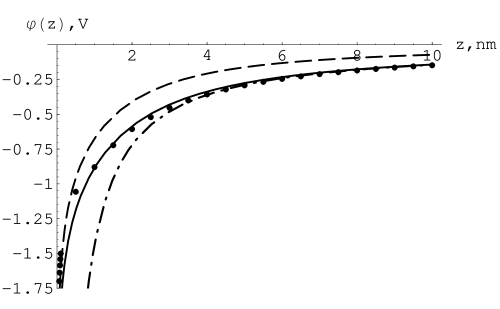
Figure 1: The $e$-$h$ interaction potentials versus the electron-hole distance $z$ for the zig-zag nanotube (28,0): dashed line - the screened one calculated by (4.5) for $T=550^{\circ}\mathrm{K}$; black circles - the screened potential (3.9); solid line - the Coulomb unscreened averaged potential (2.16); dot-dashed line - the bare Coulomb potential from (2.6)

5 Calculation results. Screening influence

Electronic structure of nanotubes, electron and hole effective masses and energy gap magnitudes were obtained in [18] within the framework of the zero-range potential method for the Bloch wave functions [19]. Using those values of effective masses and energy gaps, we have calculated the unscreened and screened $e$-$h$ interaction potentials and corresponding exciton binding energies of the ground and excited states, which either explicitly or implicitly depend on parameters of concrete semiconducting SWCNT (chirality, radius, reduced effective mass, band gap magnitude) and the temperature of medium (in Section 4). Here we present results of these calculations.

Numerically calculated values of the exciton binding energies of the ground and excited states according to (2.6) are given in table 1.

Table 1: Exciton binding energies according to (2.6).

$\mathrm{Chirality}$	$E_{\mathrm{g}},~{}\mathrm{eV}$	$\mathcal{E}_{0;\mathrm{even}},~{}\mathrm{eV}$	$\mathcal{E}_{1;\mathrm{odd}},~{}\mathrm{eV}$	$\mathcal{E}_{1;\mathrm{even}},~{}\mathrm{eV}$	$\mathcal{E}_{2;\mathrm{odd}},~{}\mathrm{eV}$
(7,0)	1.3416	-2.8343	-0.6722	-0.294	-0.168
(6,5)	1.1017	-2.9253	-0.6938	-0.3034	-0.1734
(28,0)	0.3674	-0.9484	-0.2249	-0.0983	-0.0562

These results unambiguously show that the binding energies in the even ground state for any of the selected semiconducting SWCNTs are much greater than the corresponding energy gaps in the bare Coulomb limit (2.6).

Further, the numerically calculated values of exciton binding energies at the ground and excited states according to the wave equation with the potential (2.16) are given in table 2. It can be seen from table 2, that the discrepancies with the analogous results in table 1 are more considerable for nanotubes with larger diameters, because the wave equation with the potential (2.16) tends to (2.6) if $R_{0}\rightarrow 0$.

Table 2: Exciton binding energies according to the Schrödinger equation with the potential (2.16)

$\mathrm{Chirality}$	$2R_{0},~{}\mathrm{nm}$	$\mathcal{E}_{0;\mathrm{even}},~{}\mathrm{eV}$	$\mathcal{E}_{1;\mathrm{odd}},~{}\mathrm{eV}$	$\mathcal{E}_{1;\mathrm{even}},~{}\mathrm{eV}$	$\mathcal{E}_{2;\mathrm{odd}},~{}\mathrm{eV}$
(7,0)	0.548	-2.7894	-0.5365	-0.2955	-0.1507
(6,5)	0.7468	-2.2503	-0.5071	-0.2829	-0.1488
(28,0)	2.192	-0.7567	-0.1668	-0.0928	-0.0486

We can see also from table 2 that the ground state binding energies are larger than the corresponding energy gaps even if the finiteness of nanotubes is taken into account.

The next table (table 3) shows that the exciton radii are comparable with the corresponding nanotubes diameters, thus they much greater than the nanotube lattice parameter 0.142 nm. Therefore the large radius exciton theory methods are appropriate for the treatment of the SWCNTs exciton problem.

Table 3: Exciton radii $r_{n}\sim n/2A$ in units of $2R_{0}$

$\mathrm{Chirality}$	$r_{0;\mathrm{even}}$	$r_{1;\mathrm{odd}}$	$r_{1;\mathrm{even}}$	$r_{2;\mathrm{odd}}$
(7,0)	0.4759	0.9772	1.4776	1.9545
(6,5)	0.3383	0.6948	1.05	1.3895
(28,0)	0.3556	0.73	1.1	1.46

As illustration we have calculated the binding energies for the (28,0) zig-zag nanotube with account of the nanotube dielectric function (table 4).

Table 4: Exciton binding energies for nanotube (28,0) according to (3.9) and (3.10)

$\mathrm{Chirality}$	$g_{a}$	$\mathcal{E}_{0;\mathrm{even}},~{}\mathrm{eV}$	$\mathcal{E}_{1;\mathrm{odd}},~{}\mathrm{eV}$	$\mathcal{E}_{1;\mathrm{even}},~{}\mathrm{eV}$	$\mathcal{E}_{2;\mathrm{odd}},~{}\mathrm{eV}$
(28,0)	0.6	-0.6869	-0.1799	-0.0952	-0.0501

The data from table 4 obviously show that the screening by nanotube band electrons is not enough for the ground state exciton binding energy to be less than the energy gap.

The exciton binding energies at the ground and excited states for the semiconducting (28,0) SWCNT calculated using the potential (4.5) for $T=550^{\circ}\mathrm{K}$ are listed in table 5.

Table 5: Exciton binding energies for the nanotube (28,0) according to (4.5) for $T=550^{\circ}\mathrm{K}$

$\mathrm{Chirality}$	$\kappa R_{0}$	$\mathcal{E}_{0;\mathrm{even}},~{}\mathrm{eV}$	$\mathcal{E}_{1;\mathrm{odd}},~{}\mathrm{eV}$	$\mathcal{E}_{1;\mathrm{even}},~{}\mathrm{eV}$	$\mathcal{E}_{2;\mathrm{odd}},~{}\mathrm{eV}$
(28,0)	0.38	-0.5549	-0.0642	-0.0294	-0.0133

Note, that the screened potential (4.5) may be used either for the semiconducting SWCNTs with narrow band gap (as zig-zag $(3n,0)$ SWCNTs) or for the large-diameter nanotubes (small gaps) or(and) at rather high temperatures, because only under these conditions the linear concentration $n_{0}$ of free charged particles provides a perceptible screening. At $T=550^{\circ}\mathrm{K}$ the (28,0) nanotube has approximately one free charged particle per micrometer of its length, but even at these conditions the screening by free charges of the $e$-$h$ interaction potential is much stronger than the screening by the all bound electrons of semiconducting SWCNTs (compare table 4 and table 5). Nevertheless, as it follows from the same table 5, even in this case the ground state exciton binding energy still exceeds the energy gap.

6 Discussion

In the all above examples the binding energy of the ground state of even excitons in isolated SWCNTs appeared to be much greater than the corresponding band gaps even with account of some screening effects by tubes $\pi$-electrons. This should mean that the single-electron states in SWCNTs are unstable at least in the vicinity of the energy gap with respect to formation of excitons. Such conclusion might seem doubtful though we came to it applying similar arguments as in the case of 3D large radius excitons. There are three reasons due to which a partial destruction of band electrons states in semiconducting SWCNTs in reality is either absent or inconspicuous.

First of all the account of dynamical screening, that is the frequency dependence of dielectric function, may return the all exciton levels into the band gap. This was shown in [20], where calculations of the exciton binding energy with the static dielectric function yielded also the exciton binding energy exceeding the energy gap. At the same time the self-consistent calculation with frequency dependent dielectric function gave according to [20] a universal ratio of the exciton binding energy to the energy gap depending only on the resonance integral $\gamma_{0}$ but not on the nanotube radius (it equals 0.87 if $\gamma_{0}=2.7$ eV). By [20] the exciton binding energy cannot be larger than the energy gap because of the singularity of the frequency-dependent dielectric function $\varepsilon(\omega)$ at $\omega=E_{\mathrm{g}}/\hbar$ for the frequencies, corresponding to the direct transitions between the van Hove points of the tube single-electron spectral density. However, actually this argument is true only if the exciton binding energy obtained without account of dynamical screening gets into a small vicinity of the energy of allowed transition between such points. This is because the frequency dependent SWCNT dielectric function may only then become rather great. Otherwise as it follows from results of [21] the effect of dynamical screening is too small and the exciton state with the binding energy much greater than the energy gap transforms into a long-living resonance in the continuous spectrum of electron-hole pairs with opposite quasi-momenta.

The second reason is the so-called environmental effect. In experimental works [4]-[6] (which used the methods described in [3]) investigated individual nanotubes were not in vacuum but encased in sodium dodecyl sulfate (SDS) cylindrical micelles disposed in $\mathrm{D_{2}O}$. Because of these SDS micelles, which provided a pure hydrocarbon environment around individual nanotubes, the high permittivity solvent $\mathrm{D_{2}O}$ did not reach nanotubes. However, the environment of hydrophobic hydrocarbon ”tales” $(-\mathrm{C_{12}H_{25}})$ of the SDS molecules has the permittivity greater than unity. Following the figure 1A from [3] we considered a simple model of a SWCNT in a dielectric environment: a hollow, narrow, infinite cylinder with radius $R_{0}$ in a medium with the dielectric constant $\varepsilon$ and found the potential (2.16) screened by the medium within the framework of mentioned model under the assumption about axially symmetrical charge localization at nanotube’s (here - cylinder’s) wall. The corresponding 1D screened potential $\varphi(z)$ is given by:

$$\varphi(z)=-\frac{e}{\pi R_{0}}\int\limits^{\infty}_{-\infty}\frac{I_{0}(|k|)K_{0}(|k|)\exp(\mathrm{i}kz/R_{0})}{\left[\varepsilon K_{1}(|k|)I_{0}(|k|)+I_{1}(|k|)K_{0}(|k|)\right]|k|}\ \mathrm{d}k,$$ (6.1)

where $I_{j}(|k|)$ and $K_{j}(|k|)$ are the modified Bessel functions of the order $j$ of the first and the second kind, respectively. We don’t know the exact value of dielectric constant of the pure medium, which is formed from the hydrocarbon ”tales” of the SDS molecules. But for estimates we take the dielectric constants of the substances, which are also formed from similar hydrocarbon ”tales”, e.g.: petroleum $(\varepsilon\simeq 2.1)$ or dodecane $(\varepsilon\simeq 2)$ at $293^{\circ}\mathrm{K}$ (this temperature is very close to that used in [3]-[5]), or polyethylene $(\varepsilon\simeq 2.2-2.4)$. Using the potentials (2.16) and (6.1) with $\varepsilon$ varying in the interval $2-2.4$ we have got that the ground state exciton binding energy in the nanotube (8,0) (the energy gap equals 1.415 eV [18]) is 3.06 eV in vacuum while with account of the environment it runs the interval $1.33-1.06$ eV and hence gets into the corresponding energy gap and becomes close to those in [10] (about $0.86-1$ eV), even without account of static and dynamical dielectric screening of the potential (2.16) by nanotube electrons. Remind that results on the (8,0) nanotube in [10] are in good agreement with those obtained in [5] by interpolation of experimental data for another species of nanotubes.

Further, taking the (7,5) nanotube we compare our results with the corresponding experimental data from [6], where individual SWCNTs were isolated in surfactant micelles of SDS in $\mathrm{D_{2}O}$ like in [3]. Our calculations for the (7,5) nanotube in vacuum yield 2.12 eV as the ground state exciton binding energy, while for the same tube in the SDS environment the binding energy calculated using the potential (6.1) gets into the interval $0.90-0.71$ eV (the band gap for the (7,5) tube is 1.01 eV [18]) depending on $\varepsilon$ varying from 2 to 2.4. The obtained binding energy value is not far from that of [6] $\sim 0.62$ eV even without the account of static and dynamical dielectric screening of the potential (2.16) by the nanotube electrons. There is a comparison of experimental data on the exciton binding energies in the work [6] with the corresponding theoretical results of [11]. These results are well agreed. But again, in the work [11] the interparticle potential includes screening parameter denoted as $\kappa=2$. Besides, it is asserted in [11] that the assumption of similar Coulomb parameters for SWCNTs and phenyl-based $\pi$-conjugated polymers, used in this work, gives smaller exciton binding energies for SWCNTs. All the results listed in table 1 - table 5 of our work are related only to SWCNTs in vacuum. So let us turn to the experimental work [22] which deals with optical properties (photoluminescence) of SWCNTs suspended in air (near-unit dielectric constant). As it follows from [22], the relative discrepancies between the optical transition energies obtained in [22] and those obtained in [5] are not significant (about several percents). This result could be expected, since according to the usual self-consistent field approximations the interaction of a $\pi$-electron with other electrons of a nanotube should be substantially compensated in the ground state by the interaction with the nearest ions. Evidently, the effect of this compensation is not sensitive to an environmental screening. However, for excited states such as excitons, where electrons and holes are at distances of the order of tube diameter, the environmental effect can be strong.

Note thirdly that with the advent of $N$ excitons in the tube the additional screening effect, stipulated by a rather great polarizability of excitons in the longitudinal electric field, appears. The elementary estimates show that the corresponding adding to the dielectric constant is

$$\Delta\varepsilon\approx 4\pi\frac{Ne^{2}}{\mathcal{E}_{\mathrm{b}}L},$$

where $\mathcal{E}_{\mathrm{b}}$ is the binding energy of even exciton in the ground state and $L$ is the length of a tube. We see that in the case of $N\sim 10$ per 100 nm of nanotube length $\Delta\varepsilon\simeq 1$ and therefore the lowest exciton binding energy occurs already inside the energy gap. This blocks further conversions of single-electron states into excitons. The shift of the forbidden band edges due to the transformation of some single-electron states into excitons results in some enhancement of the energy gap. As follows the optical transition energy $E_{11}$ should be blueshifted as in [22]. A coarse estimate of this shift using the elementary relation

$$\Delta E_{11}\approx\frac{\hbar^{2}\pi^{2}N^{2}}{\mu L^{2}}$$

gives $\Delta E_{11}/E_{11}\sim 10^{-2}$. If the exciton gas in tubes is unstable with respect to transition into a one-dimensional electron-hole plasma, then for the account of screening effect produced by this plasma we can use the results of Section 4. For example, for the (8,0) tube even ten charges per 100 nm of its length ($\sim 0.1\%$ of $\pi$-electrons number) reduce the ground state exciton binding energy to $0.12$ eV and thus block spontaneous transitions to the exciton states.

Thus we may conclude that the ground state of $\pi$-electrons in semiconducting SWCNTs in vacuum is formed by band electrons filling all the levels up to a certain level below the gap together with some amount of two-particle even excitations, which can form either a rare gas of excitons or electron-hole plasma. The additional screening effect induced by the exciton gas (or the one-dimensional $e$-$h$ plasma) blocks further partial destruction of single-electron states. The environmental effect may return the even exciton binding energies into the energy gap and thus may remove two-particle excitations from the ground state of $\pi$-electrons in SWCNTs.

References

- [1] Ichida M, Mizuno S, Tani Y, Saito Y and Nakamura A 1999 Exciton effects of optical transitions in single-wall carbon nanotubes J. Phys. Soc. Japan 68 3131-33
- [2] Ichida M, Mizuno S, Saito Y, Kataura H, Achiba Y and Nakamura A 2002 Coulomb effects on the fundamental optical transition in semiconducting single-walled carbon nanotubes: Divergent behavior in the small-diameter limit Phys. Rev. B 65 241407(R)
- [3] O’Connell M J et al 2002 Band gap fluorescence from individual single-walled carbon nanotubes Science 297 593-6
- [4] Bachilo S M, Strano M S, Kittrell C, Hauge R H, Smalley R E and Weisman R B 2002 Structure-assigned optical spectra of single-walled carbon nanotubes Science 298 2361-66
- [5] Weisman R B and Bachilo S M 2003 Dependence of optical transition energies on structure for single-walled carbon nanotubes in aqueous suspension: an empirical Kataura plot Nano Lett. 3 1235-8
- [6] Wang Z, Pedrosa H, Krauss T and Rothberg L 2006 Determination of the exciton binding energy in single-walled carbon nanotubes Phys. Rev. Lett. 96 047403
- [7] Ando T 1997 Excitons in carbon nanotubes J. Phys. Soc. Japan 66 1066-73
- [8] Ando T 2004 Excitons in carbon nanotubes revisited: dependence on diameter, Aharonov-Bohm flux, and strain J. Phys. Soc. Japan 73 3351-63
- [9] Spataru C D, Ismail-Beigi S, Benedict L X and Louie S G 2004 Excitonic effects and optical spectra of single-walled carbon nanotubes Phys. Rev. Lett. 92 077402
- [10] Spataru C D, Ismail-Beigi S, Benedict L X and Louie S G 2004 Quasiparticle energies, excitonic effects and optical absorption spectra of small-diameter single-walled carbon nanotubes Appl. Phys. A 78 1129-36
- [11] Zhao H and Mazumdar S 2004 Electron-electron interaction effects on the optical excitations of semiconducting single-walled carbon nanotubes Phys. Rev. Lett. 93 157402
- [12] Chang E, Bussi G, Ruini A and Molinari E 2004 Excitons in carbon nanotubes: an ab initio symmetry-based approach Phys. Rev. Lett. 92 196401
- [13] Loudon R 1959 One-dimensional hydrogen atom Am. J. Phys. 27 649-55
- [14] Cornean H D, Duclos P and Pedersen T G 2004 One dimensional models of excitons in carbon nanotubes Few-Body Systems 34 155-61
- [15] Yang X L, Guo S H, Chan F T, Wong K W and Ching W Y 1991 Analytic solution of a two-dimensional hydrogen atom. I. Nonrelativistic theory Phys. Rev. A 43 1186-96
- [16] Landau L D and Lifshitz E M 1986 Quantum Mechanics (Non-Relativistic Theory) (Course of Theoretical Physics vol 3) (Oxford: Pergamon Press) 3rd ed
- [17] Akhiezer N I and Glazman I M 1981 Theory of Linear Operators in Hilbert Space vol 2 (Monographs and Studies in Mathematics vol 10) ed E R Dawson and W N Everitt (Boston: Pitman (Advanced Publishing Program))
- [18] Tishchenko S V 2006 Electronic structure of carbon zig-zag nanotubes Low Temp. Phys. 32 953-6
- [19] Albeverio S, Gesztesy F, Høegh-Krohn R and Holden H 1988 Solvable Models in Quantum Mechanics. Texts and Monographs in Physics (New York: Springer)
- [20] Bulashevich K A, Rotkin S V and Suris R A 2003 Excitons in single-wall carbon nanotubes 11th. Int. Symp. ”Nanostructures: Physics and Technology” (June 23-28, St Petersburg, Russian Federation)
- [21] Adamyan V and Tishchenko S 2007 One-electron states and interband optical absorption in single-wall carbon nanotubes J. Phys.: Condens. Matter 19 186206
- [22] Ohno Y, Iwasaki S, Murakami Y, Kishimoto S, Maruyama S and Mizutani T 2006 Chirality-dependent environmental effects in photoluminescence of single-walled carbon nanotubes Phys. Rev. B 73 235427