Collective states in social systems with interacting
learning agents

Abstract

We consider a social system of interacting heterogeneous agents with learning abilities, a model close to Random Field Ising Models, where the random field corresponds to the idiosyncratic willingness to pay. Given a fixed price, agents decide repeatedly whether to buy or not a unit of a good, so as to maximize their expected utilities. We show that the equilibrium reached by the system depends on the nature of the information agents use to estimate their expected utilities.

1 Introduction

Individual decisions in social systems are frequently influenced by the behaviors or choices of other individuals. Besides the obvious case of fashion [28], many situations of social influence have been considered and analyzed in the literature. They range from sociological issues like the decision of attending a bar that may be crowded [2], a seminar that may have vanishing attendance [36], choosing a movie or a restaurant [3], committing crime [16], to political issues such as the decision of joining a riot [19], voting for or against a new constitution [14], etc.

The first models, proposed by Schelling [34], were aimed at demonstrating that the collective outcomes when individuals interact socially with each other may seem paradoxical – that is, intuitively inconsistent with the intentions of the individuals who generate them. In fact, the collective states that result from the aggregation of individual decisions not voluntarily coordinated, cannot be predicted by any simple counting or extrapolation of the individual preferences. Schelling [36] built simple models of social paradoxes, like the existence of racial segregation in urban neighbourhoods despite the non-racist character of the inhabitants, the death of a weekly seminar by lack of participants despite their interest on it, etc. The reason of these paradoxes is to be found in the fact that systems with interacting individuals may present multiple equilibria. These may be analyzed in a natural way in the framework of statistical physics.

Models of interacting agents facing binary decision problems have been considered within an economical framework ([5, 29, 11, 15]) after Follmer [13] first used the finite-temperature Ising model in a homogeneous external field to analyze equilibria in a two-goods market.

In this paper we consider a general model introduced in Gordon et al. [18] and Nadal et al. [26], where the interacting agents have different private willingnesses to pay, i.e. different local fields. The individual utilities are the sum of the private and the interactions terms. Interactions are assumed to be global and positive, so that utilities increase proportionally to the total fraction of buyers. Global interactions are pertinent when the individual utilities depend on decisions of remote and probably unknown individuals. This is the case of the subscription to a telephone network [31, 32], or the choice of a standard [20], where making the same decision as the majority carries advantages. Notice that this kind of aggregated data may be easily available through public information. In statistical mechanics, this model belongs to the class of mean-field ferromagnetic Random Field Ising Models.

As shown by Gordon et al. [17] when the social interactions are strong enough, the system presents multiple (Nash) zero temperature equilibria. The one that is individually and globally optimal is called Pareto-dominant equilibrium in economics. However, in contrast with physical systems where energy and entropy determine the actual thermodynamic equilibrium, none of the possible equilibria may be ruled out in social systems. Multiple equilibria bring on coordination dilemmas to the agents. The equilibrium actually reached by the system depends on the decision making dynamics.

In game theory, mostly limited to two-player games, it is usually assumed that individuals possess the skills and the information necessary to analyze the consequences of all the possible outcomes. Thus, they are able to find which is the optimal decision, and thus realize the Pareto-optimal equilibrium. However, in situations with large numbers of participants like the one considered here, or in situations of uncertainty, individuals may be unable to grasp the information necessary for coordination. In fact, they are more likely to rely on beliefs rather than on a perfectly rational reasoning to make decisions. Deviations from rationality may arise not only in situations of limited or incomplete information, but also due to human errors, different psychological attitudes with respect to risk, etc.

We are interested in situations where agents make their decisions repeatedly. In that case they may modify their beliefs by learning through past experiences. To this end we assume that each agent associates an expected surplus or payoff to buying. Once the decisions are made according to these expectations, the latter are in turn updated based on the grasped information, using a learning rule. This process is called learning upon experience in the literature. Behavioral learning is actually the subject of important theoretical studies in different disciplines, in particular in the context of game theory (see e.g. [4, 21, 22, 38]) and in ’econophysics’ (see e.g. [8, 23, 1, 27]). Quite importantly, an increasing access to empirical data allows to compare theoretical predictions with observed behaviors [7, 37].

We have studied the equilibria reached by the system for different learning rules proposed in the literature to explain outcomes in experimental economics. Following Camerer [7], we introduce a small number of parameters allowing to study all these rules within a single framework. Here we report our most interesting results, obtained through weighted belief learning and reinforcement learning. In these settings, buyers update their expectations according to their obtained surplus, while non-buyers use a degraded information. We compare results for two different information conditions. In one of them, that we call $s$-learning, the agents estimate the expected surpluses based on actual payoffs. In the other, called $\eta$-learning, they estimate them based on the fraction of individuals they expect will buy. In the latter case, agents are assumed to know the additive structure of the utility function. Our analysis is limited to populations of homogeneous learners: all the agents use the same learning rule, although they make different initial guesses. Results obtained with the standard iterative steepest ascent used to determine the local equilibria in Ising model simulations, where at each time step individuals make the best decision conditionally to the previous period outcome – a dynamics called myopic fictitious play in game theory –, serve as reference for our analysis.

We show that coordination of learners on the optimal (Nash) equilibrium, not only in the presence of multiple equilibria but even when the equilibrium is unique, is far from being the norm. In fact, fairly restrictive conditions are needed. The emerging collective state depends strongly on the values of the learning parameters, and is very sensitive to the agents’ initial beliefs. There are significant differences in the aggregate values obtained trough the simulation of both learning scenarios. Previous results corresponding to $s$-learning have been reported elsewhere [35]. The performances along the learning paths as well as the incidence of different initial conditions on the collective behaviour were thoroughly detailed. In a forthcoming paper [25] we will present an analytical study of the stationary regime attained through the learning dynamics and probabilistic decision-making.

The paper is organized as follows: in section 2, we present the agents model and its statistical mechanics equilibrium properties. In section 3, we describe the learning scenarios. We present the general settings of our simulations in section 4 and the results in section 5. Section 6 concludes the paper.

2 Model with heterogeneous interacting agents

We consider a social system of $N$ heterogeneous agents $(i=1,2,\dots,N)$ that must decide either to buy ($\omega_{i}=1$) or not ($\omega_{i}=0$) one unit of a single good at an exogenous price $P$. Following Nadal et al. [26] we assume that each agent $i$ has a willingness to pay $H_{i}$, which represents the maximal amount he is ready to pay for the good in the absence of social interactions. The values $H_{i}$ are assumed to be randomly distributed among the agents according to a probability density function of average $H$ and variance $\sigma_{H}$. In addition to this idiosyncratic term, the decisions of other agents exert an additive social influence on each individual $i$, increasing his willingness to pay if others buy. This influence is assumed to be proportional to the fraction of buyers (other than $i$):

$$\eta_{i}\equiv\frac{1}{N-1}\sum_{k\neq i}^{N}\omega_{k}.$$ (1)

The utility of buying, the surplus, for individual $i$ is:

$$S_{i}=H_{i}+J\eta_{i}-P,$$ (2)

where $J>0$, the weight of the social influence, is assumed to be the same for all the agents.

The equilibrium properties of this model have been analyzed using the mean field approximation, for different distributions of the $H_{i}$ [18, 30]. More recently, the properties for very general distributions have been determined [17]. Hereafter we briefly summarize the main results, that we illustrate for the particular case of the triangular distribution considered in our simulations. The latter allows for a complete analytical equilibrium study [30].

In the thermodynamic limit $N\to\infty$, $\eta_{i}$ in (1) and (2) may be approximated by

$$\eta\equiv\frac{1}{N}\sum_{k=1}^{N}\omega_{k}.$$ (3)

It is useful to introduce the following reduced parameters

$$x_{i}\equiv\frac{H_{i}-H}{\sigma_{H}},\,\,j\equiv\frac{J}{\sigma_{H}},\,\,\delta\equiv\frac{H-P}{\sigma_{H}},$$ (4)

where $\delta$ is the (reduced) gap between the average willingness to pay and the price. $x_{i}$ represents the (reduced) idiosyncratic preference of agent $i$. It is a random variable of zero mean and unitary variance, distributed among the population according to a probability density function (pdf) $f(x)$.

A rational agent chooses the strategy $\omega_{i}$ that maximizes his (reduced) surplus

$$s_{i}=\delta+x_{i}+j\,\eta,$$ (5)

that is:

$$\omega_{i}=\arg\max_{\omega\in\{0,1\}}\omega s_{i}.$$ (6)

In the thermodynamic limit, the fraction of buyers at equilibrium is equal to the probability of buying of the population:

$$\eta=\mathcal{P}(\delta+x_{i}+j\eta>0)=\mathcal{P}(x_{i}>-s),$$ (7)

where $s\equiv\delta+j\eta$ is the population’s average surplus. Solutions to equation (7) give the fractions of buyers at equilibrium, which depend on the parameters of the model. The properties of the system may be summarized on a phase diagram, in which the lines separating different regimes of Nash equilibria are plotted in the space of the model parameters, namely $j$ and $\delta$. The main results are that if the (reduced) strength of the social interactions $j$ is larger than a distribution dependent value $j_{B}=1/f_{max}$ ( $f_{max}$ is the maximum of the pdf), there is a range of values of $\delta$ where two different (stable) equilibria coexist: one with a large fraction of buyers, the efficient Pareto-optimal one where coordination is achieved, and another with a smaller fraction of buyers. This multiplicity is a generic property of models with social interactions [17].

In our simulations, the reduced variables $x_{i}$ are randomly distributed according to the following triangular pdf:

$$f(x)=\frac{2(2b-x)}{9b^{2}}\;\;\;{\rm if}\;\;\;-b\leq x\leq 2b,$$ (8)

with $b\equiv\sqrt{2}$. Outside the support $[-b,2b]$, $f(x)=0$. The maximum of $f(x)$ is reached at the left boundary, $f_{max}=f(-b)=2/(3b)$. The solutions to (7) are straightforward [30], and are represented as a function of $\delta$ for different values of $j$ on figure 1.

Figure 1: Demand $\eta(j;\delta)$ as a function of $\delta\equiv h-p$ for different values of $j$, for the triangular pdf (8) with maximum at $x=-b$. Notice that $\delta=0$ corresponds to $h=p$. Unstable solutions are not shown. $B$: bifurcation point, $U,L$: boundaries of the region with multiple equilibria for $j=4$.

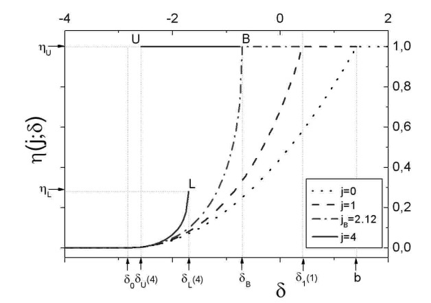
The critical value of $j$ is $j_{B}=1/f_{max}\approx 2.12$. For $j<j_{B}$, $\eta(j;\delta)$ is a single-valued function (see figure 1 for the particular value $j=1<j_{B}$). If $\delta<\delta_{0}\equiv-2b$ prices are so high with respect to the average willingness to pay of the population that there are no buyers at all ($\eta=0$), i.e. there is no market. At the other end, if $\delta>\delta_{1}(j)\equiv b-j$, prices are so low that the market saturates ($\eta=1$). These saturation effects arise because the support of $f$ is finite. For $\delta_{0}\leq\delta\leq\delta_{1}(j)$, $\eta(j;\delta)$ is a monotonically increasing function of $\delta$:

$$\eta(j;\delta)=\frac{9b^{2}}{2j}[1-\sqrt{1-\frac{4j(\delta+2b)}{9b^{2}}}]-\frac{(\delta+2b)}{j}.$$ (9)

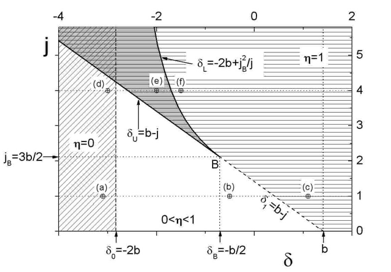
For $j>j_{B}$ there is a range of values of $\delta$, $\delta_{U}(j)\leq\delta\leq\delta_{L}(j)$ with $\delta_{L}(j)=-2b+j_{B}^{2}/j$ and $\delta_{U}(j)=b-j$ for which there are two solutions, that we denote $\eta_{U}(j;\delta)$ and $\eta_{L}(j;\delta)$, with $\eta_{U}(j;\delta)>\eta_{L}(j;\delta)$ for all the range of $\delta$ where they coexist (see $\eta(j;\delta)$ on figure 1 for $j=4>j_{B}$). More precisely, the low-$\eta$ branch, $\eta_{L}(j;\delta)$, exists for $\delta<\delta_{L}(j)$. Its dependence with $j$ and $\delta$ is the same as in equation (9). At $\delta=\delta_{L}(j)$ it reaches its largest value: $\eta_{L}(j;\delta_{L}(j))\equiv\eta_{L}(j)$. The high- $\eta$ branch exists for $\delta>\delta_{U}(j)$. In our case, it corresponds to saturation ($\eta_{U}(j;\delta)=1$). The Pareto-optimal equilibrium is $\eta_{U}(j;\delta)$, since it corresponds to the largest utility for all the buyers, which are in turn more numerous than in the equilibrium $\eta_{L}(j;\delta)$. However, the equilibrium actually reached by the system depends on the decision making process, which we study in the next section.

These results are summarized on the phase diagram of figure 2 where the saturation lines and the parameter region with two solutions (grey area) are represented.

Figure 2: Customers phase diagram for the triangular pdf (8). Grey region: coexistence of two equilibria. $\eta=0$ is an equilibrium within the obliquely-hashed region ($\delta<\delta_{0}$), $\eta=1$ (saturation) is an equilibrium within the horizontally-hashed region. Points $(a)$ to $(f)$ refer to the parameters considered in section 5.

3 Learning dynamics

We are interested in the equilibria reached by the system when the customers make their decisions repeatedly, at successive periods, based on information grasped from their past actions. We assume that at each period the agents do not know a priori the payoffs corresponding to each possible strategy. They rely on their own beliefs or estimations to make their decisions.

In the present case of binary decisions it is sufficient to estimate the difference between the payoffs expected upon buying with respect to not-buying. Thus, individuals need to estimate a single value, that we call hereafter attraction for buying, or simply attraction following Camerer [7].

We consider two different learning scenarios which differ in the kind of information assumed to be available to the customers. In the first one – that we call $s$-learning –, customers do not know the parameters nor the structure of the surplus function on which they have to make expectations. They make direct estimations of the payoffs expected upon buying (in our model the expected payoff for not buying vanishes). Starting with some initial beliefs $a_{i}(0)$, at each iteration $t$ individuals $i\in\{1,\dots,N\}$ make their decisions $\omega_{i}(t)$ for the period according to the attractions $a_{i}(t)$ and then update the latter based on the obtained payoffs $s_{i}(t)$. In the second scenario – called hereafter $\eta$ -learning –, each agent is assumed to know the gap between his idiosyncratic willingness to pay and the price ($\delta+x_{i}$) as well as the strength of the social interactions $j$. He only needs to estimate the expected fraction of buyers $\hat{\eta}_{i}(t)$, in order to determine his attraction for buying $a_{i}(t)=\delta+x_{i}+j\,\hat{\eta}_{i}(t)$.

The system is updated iteratively: at each period $t$ each agent $i$ chooses a strategy $\omega_{i}(t)$ based on his attraction $a_{i}(t)$. This choice may be probabilistic, but here we concentrate on a deterministic decision making process. Once decisions are made, attractions are updated using the grasped information. More precisely, the system evolves according to the following two-steps dynamics:

Making decisions:

each individual makes the choice that maximizes his expected payoff. Thus, if the attraction for buying is positive, the choice is $\omega_{i}(t)=1$, otherwise $\omega_{i}(t)=0$. This is called myopic best response in the literature. Since attractions are estimated payoffs,

$$\omega_{i}(t)=\Theta(a_{i}(t)).$$ (10)

where $\Theta(x)$ is the Heaviside function ($\Theta(x)=1$ if $x\geq 0$, $\Theta(x)=0$ otherwise). Notice that this deterministic decision rule depends only on the sign of the attraction but not on its magnitude. The surplus or earned payoff is then

$$s_{i}(t)=\omega_{i}(t)(\delta+x_{i}+j\eta(t))$$ (11)

where $\eta(t)$ is the actual fraction of buyers of the period. Since attractions may be inaccurate or erroneous estimations of the latter, the agents may make bad decisions and either get negative payoffs or miss positive ones.

Updating attractions:

be $z_{i}$ the quantity on which the individuals make estimations ($s_{i}$ or $\eta_{i}$, depending on the learning scenario). Individual $i$ updates $\hat{z}_{i}(t)$, the estimation at time $t$, using the information obtained as a result of his decision $\omega_{i}(t)$. The updating rules considered hereafter have the following structure:

$$\hat{z}_{i}(t+1)=(1-\mu)\,\hat{z}_{i}(t)+\mu[\Delta+(1-\Delta)\omega_{i}(t)]z_{i}(t)$$ (12)

where $0<\mu<1$ is the learning rate and $\Delta$ is a parameter ($0\leq\Delta\leq 1$) that allows to update differently $\hat{z}_{i}$ depending on the period’s decision $\omega_{i}(t)$. Notice that $z_{i}(t)$ in the right hand side of (12) is the actual value of $z(t)$ after the decision $\omega_{i}(t)$ of period $t$ is made and the corresponding payoff (if any) is earned. In particular, the learning rule obtained by setting $\Delta=1$ in (12) is known in the literature as fictitious play [7, 9]: unconditionally to $\omega_{i}(t)$, the value $\hat{z}_{i}(t+1)$ is updated using the actual value $z_{i}(t)$. If $\Delta=0$, the rule (12) gives raise to the usual reinforcement learning [12, 33], in which the estimated quantity $\hat{z}$ is updated only if $\omega_{i}(t)=1$. Another well known rule, the standard Cournot best reply [10], in which only the previous period counts, is obtained putting $\mu=1$ and $\Delta=1$ in (12). The latter corresponds to a standard parallel steepest ascent search of the (eventually local) optimum.

In the $s$-learning scenario, introducing $z_{i}(t)=s_{i}(t)$ with $s_{i}(t)$ given by equation (11), and $\hat{z}_{i}=a_{i}$ in equation (12) gives the time evolution of the attraction:

$$a_{i}(t+1)=(1-\mu)\,a_{i}(t)+\mu\,[\Delta+(1-\Delta)\omega_{i}(t)]\,s_{i}(t)$$ (13)

In the case of $\eta$-learning, $z_{i}=\eta_{i}$ and $\hat{z}_{i}=\hat{\eta}_{i}$, so that, after introduction into equation (12) and some algebra, the evolution of the corresponding attraction is:

$$a_{i}(t+1)=(1-\mu)\,a_{i}(t)+\mu\,(\delta+x_{i}+j\,[\Delta+(1-\Delta)\omega_{i}(t)]\,\eta(t))$$ (14)

Both rules coincide within the fictitious play paradigm, i.e. for $\Delta=1$.

4 General simulation-settings

In this section we present the common general settings of our simulations. Results obtained with the two different learning scenarios presented in the preceding section, namely $s$-learning and $\eta$-learning, are discussed in the next section.

4.1 Systems parameters

Simulations were done for different values of $\delta$, defined by (4). The values of $x_{i}$, the (centered) idiosyncratic component of the willingness to pay, are drawn according to the triangular pdf (8). Since this pdf is a decreasing function of $x_{i}$, there are fewer individuals with high than with low values of $x_{i}$. As a consequence, our histograms of final states as a function of $x_{i}$ have better statistics for low values than for large values of $x_{i}$.

We focus on the learning behavior for two values of the social influence weight $j$, one below, the other above, the critical value $j_{B}=3b/2\approx 2.12$ (see section 2). These are $j=1$ which has a single equilibrium for any value of $\delta$, and $j=4$, which may present two possible equilibria for the range $\delta_{U}(j)<\delta<\delta_{L}(j)$ with $\delta_{U}(4)=-2.5858$ and $\delta_{L}(4)=-1.7034$. At equilibrium, due to the boundedness of the support of the IWP, $\eta=0$ below $\delta_{0}\approx 2.83$. For $j=1$ we have $\eta=1$ above $\delta_{1}(1)\approx 0.41$, whereas for $j=4$ saturation ($\eta=1$) is a possible equilibrium for $\delta>\delta_{U}(4)$.

All the presented simulations correspond to systems with $N=1\,000$ agents, averaged over $100$ systems, i.e. corresponding to $100$ different realizations of the random idiosyncratic willingnesses to pay (IWP). We present results corresponding to synchronous (parallel) updating, where the procedure detailed in the preceding section is iterated until convergence. Results with sequential asynchronous dynamics [35] only differ in the time needed to converge, the reached equilibria being similar.

We performed thorough simulations, obtaining statistics of learning times, cumulated payoffs, etc. In this article we describe the most interesting results, which are the fractions of buyers and the distribution of attractions at convergence, because they allow to understand the differences between the different types of learning schemes.

4.2 Initial states

We assume that the agents start with some initial values of their attractions, which represent their a priori beliefs. Among the different possibilities of defining the initial beliefs, we analyze systematically three different initializations:

optimistic: in $s$-learning, the initial attractions $a_{i}(0)$ are randomly selected positive numbers in the interval $[0,1]$ for all $1\leq i\leq N$, so that the very first decision for all the agents is to buy. In $\eta$-learning, the initial values are $\hat{\eta}_{i}(0)=1$ for all $1\leq i\leq N$, so that the initial attractions are $a_{i}(0)=x_{i}+\delta+j$. Notice that in this case, the decisions of agents with $x_{i}<-j-\delta$ is not strategic: they will choose not to buy in the first period despite their optimistic guess on $\hat{\eta}_{i}(0)$, because their IWP is too small.

pessimistic: in $s$-learning, the initial attractions $a_{i}(0)$ are randomly selected negative numbers in the interval $[-1,0]$ for all $1\leq i\leq N$. At the first iteration, no agent buys. In $\eta$-learning, the initial values are $\hat{\eta}_{i}(0)=0$ for all $1\leq i\leq N$. Here, the choices of individuals with $x_{i}>-\delta$ are not strategic because their payoffs upon buying are positive independently of the choices of the other agents. Thus, their first period choice is $\omega_{i}(0)=1$.

random: in $s$-learning, the initial attractions $a_{i}(0)$ are randomly selected numbers in the interval $[-1,1]$ for all $1\leq i\leq N$. In $\eta$-learning, the initial values $\hat{\eta}_{i}(0)$ are random numbers in $[0,1]$ for all $1\leq i\leq N$. Here, agents with $x_{i}+\delta>0$ (resp. $x_{i}+\delta-j<0$) buy (resp. do not buy) unconditionally to the individual estimations $\hat{\eta}_{i}(0)$. Those with $-j<x_{i}+\delta<0$, i.e. those whose decision is actually dependent on the collective outcome, will buy only if $\hat{\eta}_{i}(0)>-(\delta+x_{i})/j$.

The two first initializations correspond to extreme cases. They lead to equilibria that are respectively upper and lower bounds to the fractions of buyers at equilibrium reached with other initializations.

5 Simulations results

We first present results obtained with myopic fictitious play, for which both learning scenarios coincide. This corresponds to the usual dynamics used in spin systems, in which at each iteration spins are aligned with their local fields. Since the interactions between agents are symmetric, the system has an underlying energy function. Thus, the dynamics has fixed point attractors, which are the equilibrium states presented in section 2. These results will serve as reference against which we compare the results of weighted belief and reinforcement learning.

5.1 Myopic fictitious play

This dynamics is achieved by putting $\Delta=1$ and $\mu=1$ in equation (12). It is called myopic because it is a response to the previous time step only: agents completely disregard older experiences and do not try to make elaborate expectations on future outcomes. Fictitious because agents are assumed to have knowledge of the values ($s$ or $\eta$) used to build their attractions independently of whether they buy or not.

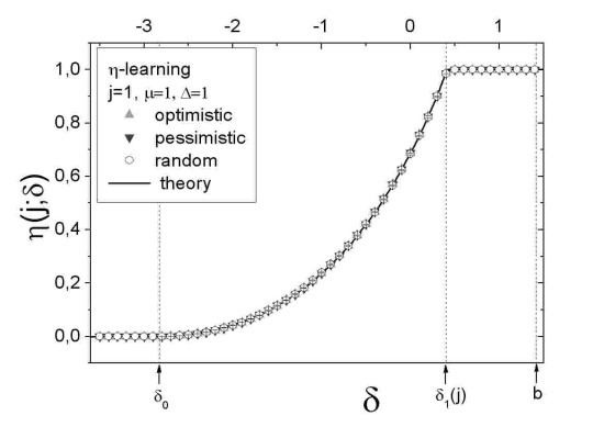
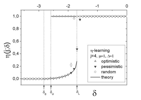
The fractions of buyers $\eta$ at equilibrium, obtained for different values of $\delta$, are presented on figure 3. Symbols correspond to simulations, the lines being the solutions to the mean field equation (7) with the triangular IWP distribution (8), represented on figure 1. In the range $0<\eta<1$ (excluding $\eta=0$ and $\eta=1$), these solutions are given by equation (9).

Figure 3: Myopic fictitious play ($\mu=1$, $\Delta=1$). $\eta$ at equilibrium versus $\delta\equiv h-p$ for $j=1$ and $j=4$. In these and all the following figures, when non visible, error bars are smaller than the symbols’ sizes. The full lines are the analytical predictions for the rational (Nash) equilibria. Numerical values of $\delta_{0}$, $\delta_{1}(j)$, $\delta_{U}(j)$ and $\delta_{L}(j)$ are given in section 4.1.

Figure 3 (left) displays results for $j=1<j_{B}$. This dynamics corresponds to steepest ascent in the states space, so that the system reaches the fixed point closest to the initial state. Since for $j=1$ there is only one fixed point for each value of $\delta$, the system converges to it independently of the initialization. For $\delta_{0}\leq\delta\leq\delta_{1}(j)$, $\eta$ is the fraction of agents that satisfy $x_{i}+\delta+j\eta>0$. In the region $\delta>\delta_{1}(j)$, these are all the agents. If $\delta<\delta_{0}$, no agent has an IWP large enough to get a positive payoff, and the equilibrium is $\eta=0$.

For $j>j_{B}$ and $\delta_{U}(j)\leq\delta\leq\delta_{L}(j)$ we expect, based on the phase diagram, that different initializations lead the system to different equilibria. Indeed, the optimistic (pessimistic) initialization systematically drives the system to the high-$\eta$ (low-$\eta$) equilibrium. Systems with random initialization end up at either of the two equilibria, depending on the precise configuration of initial states (see figure 3, right). Actually, with this initialization the distribution of $\eta$ is bimodal; this is why the averages in the coexistence region present larger variances than elsewhere. With different initial fractions of buyers, the number of simulated systems that end up at each attractor differs.

Figure 4: Myopic fictitious play ($\mu=1$, $\Delta=1$). Attractions at convergence for three different values of $\delta$, as a function of $x_{i}$. For $j=1$, the fractions of buyers are $\eta(\delta=1.1)=1$, $\eta(\delta=-0.5)=0.403$ and $\eta(\delta=-3.1)=0$. For $j=4$, $\eta(\delta=-1.5)=1$ and $\eta(\delta=-3)=0$. For $\delta=-2$ attractions converge to two different fixed points ($\eta=0.07$ and $\eta=1$), depending on the initial condition. The characters in parenthesis refer to the points in the phase diagram (figure 2).

The stationary distribution of the individual attractions $a_{i}$ of a single typical system are plotted on figures 4 against the idiosyncratic terms $x_{i}$, for different values of $\delta$ (they correspond to the equilibrium states $(a)-(f)$ in the phase diagram 2). As expected, the $a_{i}$ are the actual payoffs at equilibrium, which are proportional to $\eta$. The slope of $a_{i}$ vs. $x_{i}$ is 1, as it should, since $a_{i}=\delta+x_{i}+j\eta$, the ordinate at the origin being $\delta+j\eta$.

Results for $j=4$ and $\delta=-2$ (point (e) in the phase diagram, inside the coexistence region $\delta_{U}(4)\leq\delta\leq\delta_{L}(4)$) show the two possible outcomes, obtained through different initializations, corresponding to the two possible fixed points.

5.2 Weighted belief learning

In the weighted belief learning scenario, the information grasped by buyers has a larger weight than that of non-buyers. This scenario aims at modelizing situations where buyers have first hand knowledge of the quantities they try to estimate (payoffs or fraction of buyers) whereas individuals that do not afford the risk of buying have less faithful information. In equation (12) this is achieved whenever $0<\Delta<1$.

Figure 5: Weighted belief learning ($\mu=0.5$, $\Delta=0.5$). $\eta$ at equilibrium versus $\delta$ for $j=1$ and $j=4$, for $s$-learning (above) and $\eta$-learning (below).

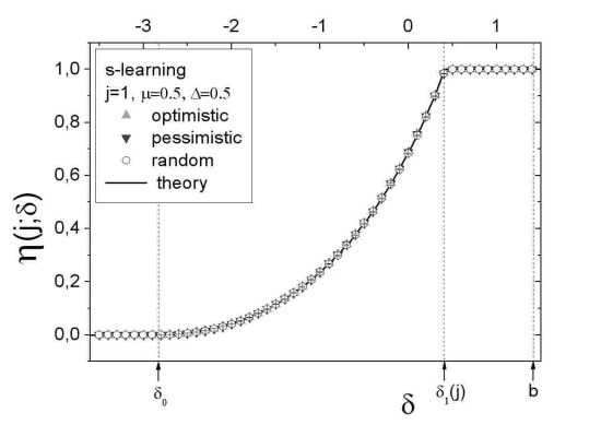
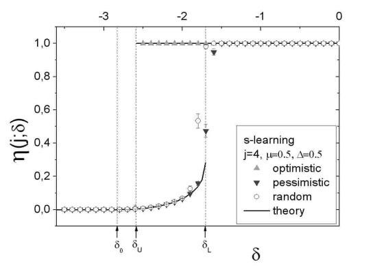
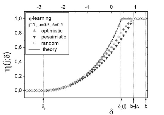
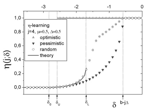
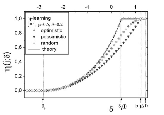
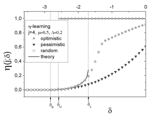
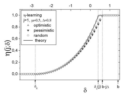
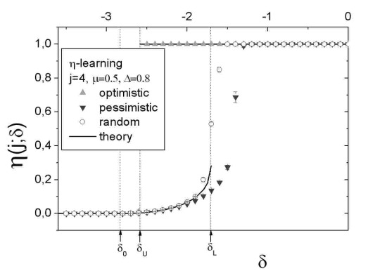
The fractions of buyers $\eta$ at convergence with $\Delta=0.5$ are plotted on figures 5. With $s$-learning, both for $j<j_{B}$ and $j>j_{B}$, equilibria are similar to those with myopic fictitious play, independently of the type of initialization, although we show later that the learned attractions are quite different. In contrast, the states reached with $\eta$-learning crucially depend on $\Delta$ being smaller than $1$. In fact, only with the optimistic initialization the agents may reach coordination on the optimal equilibrium (if it exists). With the other two initializations non-buyers systematically underevaluate the social effects by a factor $\Delta$. As a result, the $a_{i}$’s are underevaluated and the collective outcomes at equilibrium are not consistent with the phase diagram. At convergence $\eta$ is smaller than the optimal value for a large range of $\delta$ values (see figures 5). This decrease in $\eta$ is most dramatic with the pessimistic initialization. Since with the random initialization there are more buyers than with the pessimistic initialization from the beginning, more individuals can correctly estimate their surpluses, and the collective state at equilibrium has systematically a larger $\eta$ than when starting with the pessimistic initialization.

Figure 6: Weighted belief learning ($\mu=0.5$): dependence of $\eta$-learning on $\Delta$: $\eta$ at equilibrium versus $\delta$ for $j=1$ and $j=4$ with $\Delta=0.2$ (above) and $\Delta=0.8$ (below).

For smaller values of $\Delta$, the misestimations of the social terms are even more conspicuous, leading the population to inefficient equilibria with low fractions of buyers for a larger range of $\delta$ values (see figures 6, $\Delta=0.2$). Conversely, when $\Delta$ is larger, the actual and the estimated $\eta$ are closer to each other, giving results closer to those of fictitious play (see figures 6, $\Delta=0.8$). In the limit $\Delta\to 1$ we obtain the results of section 5.1. The case $\Delta=0$ is considered in the next section.

Figure 7: Weighted belief learning ($\mu=0.5$, $\Delta=0.5$). Attractions at convergence for three values $\delta$, as a function of $x_{i}$. Above, for $s$-learning: $\eta(j=1,\delta=1.1)=1$, $\eta(j=1,\delta=-0.5)=0.403$ and $\eta(j=1,\delta=-3.1)=0$. For $j=4$, when $\delta=-2$ attractions converge to two different fixed points (with $\eta=0.078$ and $\eta=1$), depending on the initial condition) whereas $\eta=1$ for $\delta=-1.5$ and $\eta=0$ for $\delta=-3$. Below, for $\eta$-learning: $\eta(j=1,\delta=1.1)=1$, $\eta(j=1,\delta=-0.5)=0.382$ and $\eta(j=1,\delta=-3.1)=0$. For $j=4$, when $\delta=-2$ attractions converge to two different fixed points (with $\eta=0.03$ and $\eta=1$, depending on the initial condition), whereas $\eta(j=4,\delta=-1.5)=0.62$ and $\eta(j=4,\delta=-3=0$ .

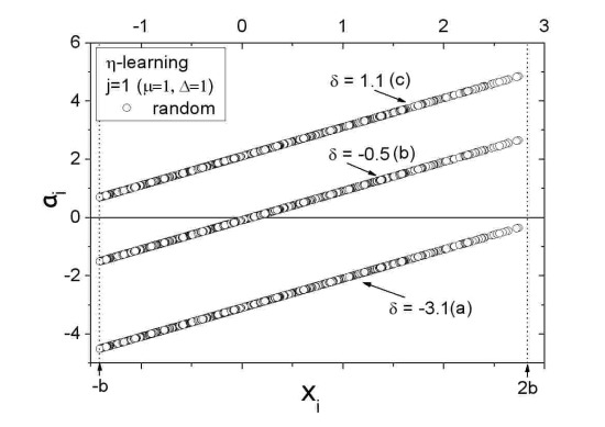
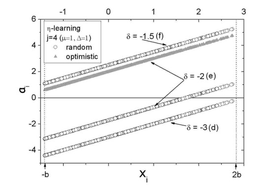
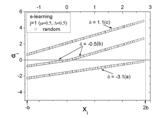
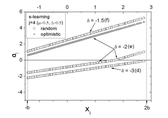
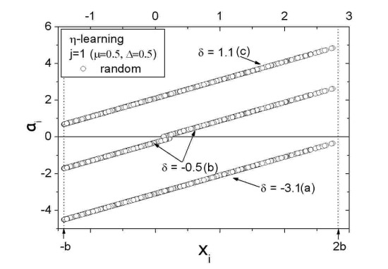
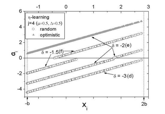
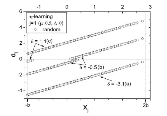
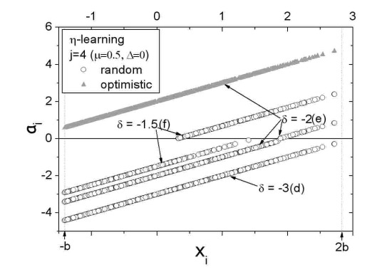
The individual attractions at convergence of a representative system are represented against the individual idiosyncratic terms $x_{i}$ on figures 7, for $j=1$ and $j=4$ and for different values of $\delta$. In contrast with myopic fictitious play, the slope of the attractions obtained with $s$-learning depends on whether individuals are buyers or not: for non-buyers the slope is $\Delta$ whereas it is $1$ for buyers, as may be seen on the upper figures 7.

In the case of $\eta$-learning it is clear from the updating rule (14) that the attractions as a function of $x_{i}$ have a slope $1$. However, because $\Delta<1$, both with the pessimistic and the random initializations the fractions of non-buyers when $j=1$ for $\delta$ in the region $\delta_{1}(j)<\delta<b-j\Delta$ (see figure 5) do not reach the saturation level expected from the phase diagram. The non-buyers are agents whose initial estimations $\hat{\eta}_{i}(0)$ determined negative attractions. When the correcting term $j\Delta\eta$ does not allow to compensate a negative value of $\delta+x_{i}$, these agents persist in non buying.

When $j=4$, for $\delta>\delta_{L}(j)$ there is a fraction of the population that does not buy, due to same reason as for $j<j_{B}$. This is why for $\delta=-1.5>\delta_{L}(4)$, where saturation is expected on the basis of the phase diagram, we obtain $\eta<1$ with either random or pessimistic initializations. Like for $j=1$, here also saturation is reached independently of the initial state only for $\delta>b-j\Delta$.

5.3 Reinforcement learning

Figure 8: Reinforcement learning ($\mu=0.5$, $\Delta=0$). Attractions at convergence for three values of $\delta$, as a function of $x_{i}$. $s$-learning (above): the fractions of buyers for $j=1$ are $\eta(j=1,\delta=1.1)=0.52$, $\eta(j=1,\delta=-0.5)=0.203$ and $\eta(j=1,\delta=-3.1)=0$. For $j=4$, $\delta=-2$, attractions converge to two different fixed points (with $\eta=0.022$ and $\eta=1$, depending on the initial condition), whereas $\eta(j=4,\delta=-1.5)=0.095$ and $\eta(j=4,\delta=-3)=0$. $\eta$-learning (below): $\eta(j=1,\delta=1.1)=0.985$, $\eta(j=1,\delta=-0.5)=0.374$ and $\eta(j=1,\delta-3.1)=0$. For $j=4$, $\delta=-2$ attractions converge to two different fixed points ($\eta=0.03$ and $\eta=1$, depending on the initial condition), whereas $\eta(j=4,\delta=-1.5)=0.294$ and $\eta(j=4,\delta=-3)=0$.

In reinforcement learning, only agents that buy are assumed to have the information necessary to estimate their attractions. In equation (12) this is achieved with $\Delta=0$. This learning paradigm is also called stimulus-response or rote learning in behavioral psychology [6]. It aims at modelizing risk-averse individuals that refrain from buying from the start, independently of the posted price. As we see in the following, such behaviours may hinder the emergence of the Pareto-optimal equilibrium, where the payoffs are optimal for all the agents, for a large range of values of $\delta$.

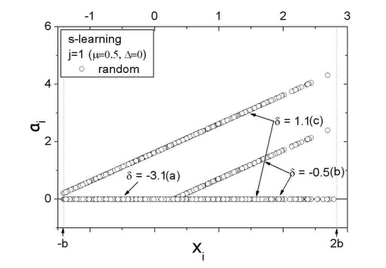
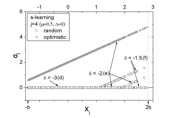
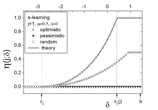
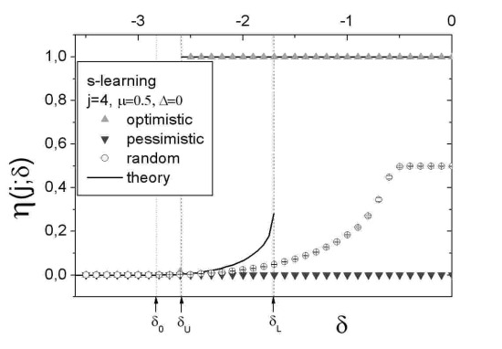
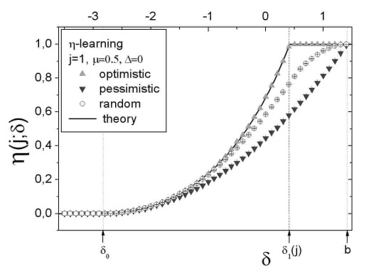
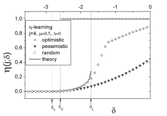
Like in weighted belief learning, the system’s behavior with reinforcement learning strongly depends on the initial states. In fact, only individuals with $a_{i}(0)>0$ can actually learn from experience because their first decision is to buy. Therefore, the attractions of buyers (but only these) converge to the actual payoffs $s_{i}=x_{i}+\delta+j\eta$, both with $\eta$- and $s$-learning. Their values of $a_{i}$ at convergence present a slope $1$ as a function of $x_{i}$. With $s$-learning non-buyers (whose attractions are negative) cannot use the information carried by the forgone payoffs. These agents decrease iteratively by a factor $1-\mu$ the absolute values of $a_{i}$ at each step of the learning process. Attractions keep thus their negative signs: the corresponding individuals persist in state $\omega_{i}=0$ and the attractions of non-buyers converge to $a_{i}=0$ whatsoever the value of $x_{i}$. In figure 8 the corresponding $a_{i}$ vs $x_{i}$ present a vanishing slope, and there are individuals with $a_{i}=0$ evenly distributed over the $x_{i}$ axis. Notice that even when $\delta$ is large enough (low enough price) to allow everybody get positive payoffs, at equilibrium there remain non-buyers with vanishing attractions independently of their value of $x_{i}$. On figure 9, the fraction of buyers $\eta$ (with random initialization) is seen to be systematically smaller than the fraction expected from the phase diagram. Since in our random initialization setting the initial values $a_{i}(0)$ are selected with equal probabilities of being positive or negative, the initial fraction of buyers is $\eta(0)=0.5$. Since those who begin with $a_{i}(0)<0$ are unable to change their mind, the upper bound to $\eta$ is $1/2$, as is seen in the upper figures 9. For the same reasons, with the pessimistic initialization nobody buys independently of $\delta$. Only with the optimistic initialization all the individuals can learn and make correct estimations of their payoffs: the corresponding curves $\eta$ vs. $\delta$ are similar to those with myopic best response.

Figure 9: Reinforcement learning ($\mu=0.5$, $\Delta=0$). $\eta$ at equilibrium versus $\delta\equiv h-p$ for $j=1$ and $j=4$, for $s$-learning (above) and $\eta$-learning (below).

With $\eta$-learning the behavior is closer to that of weighted belief learning: the curves $\eta(j;\delta)$ follow the same trends as in figures 6. The attractions of buyers (non-buyers) converge to $a_{i}=\delta+x_{i}+j\eta$ ($a_{i}=\delta+x_{i}$). The range of $x_{i}$ values where individuals may have different $a_{i}$ even if they have similar $x_{i}$ is obtained like with weighted belief learning, putting $\Delta=0$ in the equations. This gives $-\delta-j\eta<x_{i}<-\delta$. This is illustrated on figures 8 (below), and explains why here also the values of $\eta$ at convergence are systematically smaller (or equal) to those expected at the Nash equilibrium, as may be seen on figures 9 (below). Notice that with $\eta$-learning, even if non-buyers do not use the information about $\eta$, they may still buy provided that $x_{i}+\delta>0$, independently of the initial guess $\eta_{i}(0)$. This is why $\eta$ may be larger than with $s$-learning at convergence, see figure 9 (below), and even reach saturation provided $\delta$ is large enough. The same argument as in the preceding section shows that saturation can be reached only if $\delta>b$.

6 Discussion and Conclusion

It is interesting to compare the results obtained with weighted belief learning to those with reinforcement learning. In both cases, the equilibrium values of the attractions may be calculated by replacing $a_{i}(t)$, $\eta(t)$, $\omega_{i}(t)$ in (13) and (14) by their asymptotic values $a_{i}$, $\eta$ and $\omega_{i}$. With $s$-learning these are $a_{i}=[\Delta+(1-\Delta)\omega_{i}]s_{i}$: the attractions of buyers converge to $a_{i}=s_{i}$, i.e. they estimate correctly their expected surplus. Non-buyers estimate $a_{i}=\Delta s_{i}$. With $\eta$-learning we have $a_{i}=x_{i}+\delta+j\eta[\Delta+(1-\Delta)\omega_{i}]$. Thus buyers also correctly estimate their expected surplus, and non-buyers underestimate it, since their attractions converge to $a_{i}=x_{i}+\delta+j\Delta\eta$.

With weighted belief $s$-learning, the agents always estimate the right sign of the attraction independently on whether they are buyers or non-buyers, so that the system converges to the theoretical Nash equilibrium despite the incorrect estimations by non-buyers. This is not true for reinforcement learning ($\Delta=0$), because in this case the attractions of non-buyers converge to $a_{i}=s_{i}\Delta=0$. As a result, at equilibrium we expect fewer buyers than with weighted belief learning, because with reinforcement learning individuals that have initial negative attractions persist in non-buying even if they could obtain positive payoffs.

With $\eta$-learning, like with $s$-learning, buyers’ asymptotic attractions converge to the actual surpluses both with weighted belief and with reinforcement learning: $a_{i}=s_{i}$. Non-buyers’ surplus estimations converges to $a_{i}=s_{i}-(1-\Delta)j\eta$, which may be negative even if $s_{i}>0$. Therefore, in contrast with $s$-learning, weighted belief $\eta$ -learning may fail to reach the theoretical Nash equilibria. With reinforcement learning, on the other hand, $\eta$-learning may be more performant than $s$-learning, since non-buyers’ estimations converge to $a_{i}=\delta+x_{i}$, i.e., they disregard the social component of the surplus but take into account correctly their idiosyncratic preferences. Therefore, the fraction of buyers increases with $\delta$, without getting stuck at a value determined only by the initial conditions, as happens with $s$-learning.

The comparison of $s$- and $\eta$-learning with the same parameters shows that with weighted belief learning, $\eta$-learning converges to fewer buyers than $s$-learning, because in the latter case the sign of the surplus is correctly estimated. This is a rather counterintuitive result, since individuals using $s$-learning have a poorer knowledge of the payoff structure. On the other hand, $\eta$-learning allows to get closer to the theoretical Nash equilibria because the agents know their preferences, and only misestimate the fraction of buyers. To summarize, with reinforcement learning the quality of the equilibria with the two learning scenarios is inversed with respect to the one in weighted belief learning. In $\eta$ -learning, agents with the a priori knowledge about $x_{i}$ and $j$ drive the system through learning to states with larger fractions $\eta$ than with $s$-learning, where agents do not have this a priori information.

We only considered $0\leq\Delta\leq 1$, implying that non-buyers may only underestimate the learned quantity (be it the forgone payoff or the fraction of buyers). Values $\Delta>1$ allow to modelize the non-buyers regret about their chosen strategy. These $\Delta$ values can only lead to overestimations of the learned term, helping non-buyers to increase faster their attractions for buying. The result would be an acceleration of convergence. Since buyers make correct estimations, we expect that, except for reinforcement $s$-learning, the final states be the same as with fictitious play. With reinforcement $s$-learning, the results would be the same as those presented here.

To conclude, our results show that systems with interacting rational agents with limited information may not reach the theoretical Nash equilibria, even when these are unique. If the social interactions are so strong that there are multiple Nash equilibria, the resulting collective state is very sensitive to the agents’ initial guesses of the opportunity of buying.

We restricted our simulations to systems where all the agents use the same learning rule. Further investigations should consider mixtures of different kinds of learners.

Our agents used deterministic learning rules. One drawback is that their decisions are independent of the magnitude of the attraction: only its sign matters. Probabilistic decision rules, where the uncertainty of the choice is larger the closer the attraction to $0$, have been studied in a related model where adaptive customers have to choose between different sellers [37, 27], in a particular context where fictitious play is not possible. There, the existence of multi-equilibria is shown to lead to a transition between an unfaithful and a faithful behaviour (customers going to different sellers in the first case, and preferring one particular seller in the other case). Within our general framework we have studied the adaptive dynamics with probabilistic decision rules. A typical result is that the population reaches states in which decisions fluctuate close to the average ones. This stationary regime is in general close to the ‘quantal response equilibrium’ [24] described in economics. In addition, a more complex stationary state can be obtained when the choice uncertainty is strong enough. A detailed analysis of the collective behaviour under such probabilistic decision rules will be presented elsewhere [25].

References

- [1] M. Andrecut and M. K. Ali. Q learning in the minority game. Physical Review E, 64:067103, (2001).
- [2] W. B. Arthur. El farol. Amer. Econ. Review, 84:406, (1994).
- [3] G. S. Becker. A note on restaurant pricing and other examples of social influences on price. The Journal of Political Economy, 99:1109–1116, (1991).
- [4] Michel Benaim and Morris W Hirsch. Learning processes, mixed equilibria and dynamical systems arising from fictitious play in perturbed games. Games and Economic Behavior, 29:36–72, 1999.
- [5] L. E. Blume. The statistical mechanics of strategic interaction. Games and Economic Behavior, 5:387–424, (1993).
- [6] R. Bush and F. Mosteller. Stochastic models for learning. Wiley, (1955).
- [7] C. F. Camerer. Behavioral Game Theory. Princeton University Press, Princeton, New Jersey, (2003).
- [8] Damien Challet, Matteo Marsili, and Yi-Cheng Zhang. Minority Games: Interacting agents in financial markets. Oxford Univ Press, 2004.
- [9] Y. W. Cheung and J.W. Friedman. Individual learning in normal form games: Some laboratory results. Games and Economic Behavior, 19:46–76, (1997).
- [10] A. Cournot. Recherches sur les principes mathematiques de la theorie des richesses. N. Bacon, Trans. [Researches in the mathematical principles of the theory of wealth]. London: Haffner, (1960).
- [11] S. N. Durlauf. Statistical mechanics approaches to socioeconomic behavior. In B. Arthur, S. N. Durlauf, and D. Lane, editors, The Economy as an Evolving Complex System II. Santa Fe Institute Studies in the Sciences of Complexity, Volume XVII, Addison-Wesley Pub. Co, (1997).
- [12] I. Erev and A. E. Roth. Predicting how people play games: reinforcement learning in experimental games with unique, mixed strategy equilibria. The American Economic Review, 88:4:848–881, (1998).
- [13] H. Föllmer. Random economies with many interacting agents. Journal of Mathematical Economics, 1:1:51–62, (1974).
- [14] S. Galam, Y. Gefen, and Y. Shapir. Sociophysics: A mean behavior model for the process of strike. Mathematical Journal of Sociology, 9:1–13, (1982).
- [15] E. Glaeser and J. A. Scheinkman. Non-market interactions. In M. Dewatripont, L.P. Hansen, and S. Turnovsky, editors, Advances in Economics and Econometrics: Theory and Applications, Eight World Congress. Cambridge University Press, (2003).
- [16] E. L. Glaeser, B. Sacerdote, and J. A. Scheinkman. Crime and social interactions. Quarterly Journal of Economics, CXI:507–548, (1996).
- [17] M. B. Gordon, J.-P. Nadal, D. Phan, and V. Semeshenko. Discrete choices under social influence: generic properties. Submitted, (2007) Working paper: http://halshs.archives-ouvertes.fr/halshs-00135405.
- [18] M. B. Gordon, J.-P. Nadal, D. Phan, and J. Vannimenus. Seller’s dilemma due to social interactions between customers. Physica A, 356, Issues 2-4:628–640, (2005).
- [19] M. Granovetter. Threshold models of collective behavior. American Journal of Sociology, 83(6):1360–1380, (1978).
- [20] M. Katz and C. Shapiro. Technology adoption in the presence of network externalities. Journal of Political Economy, 94:822–41, (1986).
- [21] A. Kryazhimskii, Y. Kaniovski, and P. Young. Adaptive dynamics in games played by heterogeneous populations. Games and Economic Behavior, 31:50–96, (2000).
- [22] J.F. Laslier, R. Topol, and B. Walliser. A behaviorial learning process in games. Games and Economic Behavior, 37:”340–366”, (2001).
- [23] Matteo Marsili, Damien Challet, and Riccardo Zecchina. Exact solution of a modified el farol’s bar problem: Efficiency and the role of market impact. Physica A: Statistical Mechanics and its Applications, 280, Issues 3-4:522–553, 2000, arXiv:cond-mat/9908480v3.
- [24] R. D. McKelvey and T. R. Palfrey. Quantal response equilibria for normal games. Games and Economic Behavior, 7:6–38, (1995).
- [25] J.-P. Nadal, M. B. Gordon, and V. Semeshenko. in preparation.
- [26] J.-P. Nadal, D. Phan, M. B. Gordon, and J. Vannimenus. Multiple equilibria in a monopoly market with heterogeneous agents and externalities. Quantitative Finance, 5(6):557–568, (2006).
- [27] J.-P. Nadal, G. Weisbuch, O. Chenevez, and A. Kirman. A formal approach to market organisation: Choice functions, mean field approximation and maximum entropy principle. In J. Lesourne and A. Orl an, editors, Advances in Self-Organization and Evolutionary Economics, pages 149–159. Economica, London, (1998).
- [28] Shoichiro Nakayama and Yasuyuki Nakamura. A fashion model with social interaction. Physica A: Statistical and Theoretical Physics, 337(3-4):625–634, (2004).
- [29] A. Orléan. Bayesian interactions and collective dynamics of opinion: Herd behaviour and mimetic contagion. Journal of Economic Behavior and Organization, 28:257–274, (1995).
- [30] D. Phan and V. Semeshenko. Equilibria in models of binary choice with heterogeneous agents and social influence. submitted to European Journal of Economic and Social Systems, , (2007).
- [31] J. Rohlfs. A theory of interdependent demand for a communications service. The Bell Journal of Economics and Management Science, 5 (1):16–37, (1974).
- [32] J. Rohlfs. Bandwagon Effects in High Technology Industries. MIT Press, (2001).
- [33] R. Sarin and F. Vahid. Predicting how people play games: a simple dynamic model of choice. Games and Economic Behavior, 34:104–122, (2001).
- [34] T. S. Schelling. Dynamic models of segregation. Journal of Mathematical Sociology, 1:143–186, (1971).
- [35] V. Semeshenko, M. B. Gordon, J.-P. Nadal, and D. Phan. Choice under social influence: effects of learning behaviors on the collective dynamics. Book Chapter in Cognitive Economics: New Trends, 280:177–203, (2006).
- [36] Schelling T.S. Micromotives and Macrobehavior. W.W. Norton and Co, N.LY., (1978).
- [37] G. Weisbuch, A. Kirman, and D. Herreiner. Market organisation and trading relationships. Working paper 1996, published in: The Economic Journal, Volume 110 Issue 463:411–462, (2000).
- [38] H. P. Young. Bounded rationality and learning. on the limits of rational learning. European Economic Review, 46:791–799, (2002).