Quasi Equilibrium Grid Algorithm: geometric construction for model reduction

Eliodoro Chiavazzo chiavazzo@lav.mavt.ethz.ch Iliya V. Karlin karlin@lav.mavt.ethz.ch Aerothermochemistry and Combustion Systems Laboratory (LAV), ETHZ CH-8092 Zurich, Switzerland.
Abstract

The Method of Invariant Grid (MIG) is an iterative procedure for model reduction in chemical kinetics which is based on the notion of Slow Invariant Manifold (SIM) [1]-[4]. Important role, in that method, is played by the initial grid which, once refined, gives a description of the invariant manifold: the invariant grid. A convenient way to get a first approximation of the SIM is given by the Spectral Quasi Equilibrium Manifold (SQEM) [1]-[2]. In the present paper, a flexible numerical method to construct the discrete analog of a Quasi Equilibrium Manifold, in any dimension, is presented. That object is named Quasi Equilibrium Grid (QEG), while the procedure Quasi Equilibrium Grid Algorithm. Extensions of the QEM notion are also suggested. The QEG is a numerical tool which can be used to find a grid-based approximation for the locus of minima of a convex function under some linear constraints. The method is validated by construction of one and two-dimensional grids for model hydrogen oxidation reaction.

keywords:
Chemical kinetics , model reduction , invariant manifold , entropy , nonlinear dynamics , Lagrange multipliers method , variational problem.

,

1 Introduction

Relaxation of complex systems is often characterized by a fast dynamics during a short initial stage, while the remaining period lasts much longer and it evolves along low-dimensional surfaces in the phase space known as Slow Invariant Manifolds (SIM). In that scenario, a simplified macroscopic description of a complex system can be attained by extracting only the slow dynamics and neglecting the fast one. For this reason, much effort was spent to develop model reduction methods (the Method of Invariant Grid (MIG) [1, 2, 3, 4], the Intrinsic Low Dimensional Manifold method (ILDM) [9, 10], the Computational Singular Perturbation method (CSP) [11, 12, 13], etc.) based on the notion of SIM. The introduction of a convex Lyapunov function G𝐺G, whenever the complex system is supported by such a function, also proves to be very helpful in model reduction [4, 8]. Indeed, it was shown that, through a G𝐺G function, good approximations of the SIM can be found (e.g. by constructing the Spectral Quasi Equilibrium Manifold - SQEM - or the Symmetric Entropic Intrinsic Low Dimensional Manifold - SEILDM - [1, 2]) and refined by some efficient MIG iterations. Moreover, it has been shown that the notion of QEM is also very useful in different fields. For example, it was used in the implementation of Lattice Boltzmann schemes [6, 7]. Construction of a QEM is analytically possible by using the Lagrange multipliers method. However, its implementation becomes too complicated as soon as the number of variables of the problem becomes large: efficient methods, for constructing large dimensional QEM, are still missing. Therefore, in the present paper the notion of Quasi Equilibrium Grid (QEG) will be introduced, as a discrete analog of QEM, and a constructive algorithm, applicable in any dimension, will be developed. The procedure suggested proves to be a very flexible tool, so it is possible to get some other SIM approximations, all based on the previous algorithm, even more accurate than the QEG itself.

2 Paper organization

The paper is organized as follows. In Section 3, some basic notions are outlined: in particular, the general equations of dissipative reaction kinetics are reviewed, in the notations which are used throughout the paper. At the end of that Section, the Method of Invariant Grid (MIG) and the notion of thermodynamic projector are briefly discussed (Section 3.2). In Section 4, the QEM definition and its geometrical interpretation is given, while in Section 5 the 1D Quasi Equilibrium Grid Algorithm is presented. That algorithm is also illustrated, by means of an example, in Section 6. The 1D Algorithm extension to multi-dimensional grids is developed in Section 7. In particular, two possible extension strategies are analyzed: the straightforward extension (Section 7.1) and, by following the general idea given in [3], the flag extension (Section 7.2). Here, it is also shown how the flexibility of the flag extension allows to get SIM approximation which is better than the Spectral-QEG (Section 7.3): the notions of Guided-QEG and Symmetric Entropic Guided-QEG are introduced. An illustrative example, in Section 8, shows how those different extension techniques work in practice. In order to find out how accurate is their SIM description, they are also compared on the base of the invariance defect (Section 8.3). Finally, results are discussed in Section 9.

3 Theoretical background

3.1 Dissipative reaction kinetics

In a closed system with n chemical species A1,,Ansubscript𝐴1subscript𝐴𝑛A_{1},...,A_{n}, participating in a complex reaction, a generic reversible reaction step can be written as a stoichiometric equation:

αs1A1++αsnAnβs1A1++βsnAn,subscript𝛼𝑠1subscript𝐴1subscript𝛼𝑠𝑛subscript𝐴𝑛subscript𝛽𝑠1subscript𝐴1subscript𝛽𝑠𝑛subscript𝐴𝑛\alpha_{s1}A_{1}+...+\alpha_{sn}A_{n}\rightleftharpoons\beta_{s1}A_{1}+...+\beta_{sn}A_{n}, (1)

where s is the reaction index, s=1,,r𝑠1𝑟s=1,...,r (r steps in total), and the integers αsisubscript𝛼𝑠𝑖\alpha_{si} and βsisubscript𝛽𝑠𝑖\beta_{si} are stoichiometric coefficients of the step s. For each reaction step, we can introduce n-component vectors 𝜶ssubscript𝜶𝑠\mbox{\boldmath$\alpha$}_{s} and 𝜷ssubscript𝜷𝑠\mbox{\boldmath$\beta$}_{s}, with components αsisubscript𝛼𝑠𝑖\alpha_{si} and βsisubscript𝛽𝑠𝑖\beta_{si}, and the stoichiometric vector 𝜸ssubscript𝜸𝑠\mbox{\boldmath$\gamma$}_{s}=𝜷ssubscript𝜷𝑠\mbox{\boldmath$\beta$}_{s}-𝜶ssubscript𝜶𝑠\mbox{\boldmath$\alpha$}_{s}. For every Aisubscript𝐴𝑖A_{i} the extensive variable Nisubscript𝑁𝑖N_{i} describes the number of particles of that species. If V is the volume, then the concentration of Aisubscript𝐴𝑖A_{i} is ci=Ni/Vsubscript𝑐𝑖subscript𝑁𝑖𝑉c_{i}=N_{i}/V. Dynamics of the species concentration according to the stoichiometric mechanism (1) reads:

N˙=VJ(c),J(c)=s=1r𝜸sWs(c),˙N𝑉Jcmissing-subexpressionJcsuperscriptsubscript𝑠1𝑟subscript𝜸𝑠subscript𝑊𝑠cmissing-subexpressionmissing-subexpressionmissing-subexpressionmissing-subexpressionmissing-subexpressionmissing-subexpressionmissing-subexpressionmissing-subexpressionmissing-subexpressionmissing-subexpressionmissing-subexpressionmissing-subexpressionmissing-subexpressionmissing-subexpressionmissing-subexpressionmissing-subexpressionmissing-subexpression\begin{array}[]{*{20}c}{\dot{\emph{{N}}}=V\emph{{J}}(\emph{{c}}),}&{}\hfil&{\emph{{J}}(\emph{{c}})=\sum\nolimits_{s=1}^{r}{\mbox{\boldmath$\gamma$}_{s}W_{s}(\emph{{c}}),}}\\ \end{array} (2)

where dot denotes the time derivative and Ws(c)subscript𝑊𝑠cW_{s}(\emph{{c}}) is the reaction rate function of the step s. In particular, the polynomial form of the reaction rate function is provided by the mass action law:

Ws(c)=Ws+(c)Ws(c)=ks+(T)i=1nciαiks(T)i=1nciβi,subscript𝑊𝑠csuperscriptsubscript𝑊𝑠csuperscriptsubscript𝑊𝑠csuperscriptsubscript𝑘𝑠𝑇superscriptsubscriptproduct𝑖1𝑛superscriptsubscript𝑐𝑖subscript𝛼𝑖superscriptsubscript𝑘𝑠𝑇superscriptsubscriptproduct𝑖1𝑛superscriptsubscript𝑐𝑖subscript𝛽𝑖W_{s}(\emph{{c}})=W_{s}^{+}(\emph{{c}})-W_{s}^{-}(\emph{{c}})=k_{s}^{+}(T)\prod\limits_{i=1}^{n}{c_{i}^{\alpha_{i}}-}k_{s}^{-}(T)\prod\limits_{i=1}^{n}{c_{i}^{\beta_{i}},} (3)

where ks+(T)superscriptsubscript𝑘𝑠𝑇k_{s}^{+}(T) and ks(T)superscriptsubscript𝑘𝑠𝑇k_{s}^{-}(T) are the constants of the direct and of the inverse reactions rates of the step s respectively. The most popular form of their dependence is given by the Arrhenius equation:

ks±(T)=as±Tbs±exp(Ss±/kB)exp(Hs±/kBT).superscriptsubscript𝑘𝑠plus-or-minus𝑇superscriptsubscript𝑎𝑠plus-or-minussuperscript𝑇superscriptsubscript𝑏𝑠plus-or-minussuperscriptsubscript𝑆𝑠plus-or-minussubscript𝑘𝐵superscriptsubscript𝐻𝑠plus-or-minussubscript𝑘𝐵𝑇k_{s}^{\pm}(T)=a_{s}^{\pm}T^{b_{s}^{\pm}}\exp(S_{s}^{\pm}/k_{B})\exp(-H_{s}^{\pm}/k_{B}T).

In the latter equation, as±superscriptsubscript𝑎𝑠plus-or-minusa_{s}^{\pm},bs±superscriptsubscript𝑏𝑠plus-or-minusb_{s}^{\pm} are constants and Hs±superscriptsubscript𝐻𝑠plus-or-minusH_{s}^{\pm}, Ss±superscriptsubscript𝑆𝑠plus-or-minusS_{s}^{\pm} activation enthalpies and entropies respectively. The rate constants are not independent. Indeed, the principle of detail balance gives a relation between these quantities:

Ws+(ceq)=Ws(ceq),s=1,,r,superscriptsubscript𝑊𝑠superscriptc𝑒𝑞superscriptsubscript𝑊𝑠superscriptc𝑒𝑞missing-subexpressionfor-all𝑠1𝑟missing-subexpressionmissing-subexpressionmissing-subexpressionmissing-subexpressionmissing-subexpressionmissing-subexpressionmissing-subexpressionmissing-subexpressionmissing-subexpressionmissing-subexpressionmissing-subexpressionmissing-subexpressionmissing-subexpressionmissing-subexpressionmissing-subexpressionmissing-subexpressionmissing-subexpression\begin{array}[]{*{20}c}{W_{s}^{+}(\emph{{c}}^{eq})=W_{s}^{-}(\emph{{c}}^{eq}),}&{}\hfil&{\forall s=1,...,r,}\\ \end{array} (4)

where the positive vector ceq(T)superscriptc𝑒𝑞𝑇\emph{{c}}^{eq}(T) is the equilibrium of the system (2). In order to obtain a closed system of equations, one should supply an equation for the volume V. For an isolated system the extra-equations are U,V=constUVconst\emph{U},\emph{V}=\emph{const} (where U is the internal energy), for an isochoric isothermal system we get V,T=constVTconst\emph{V},\emph{T}=\emph{const}, and so forth. For example, equation (2) in the latter case simply takes the form:

c˙=s=1r𝜸sWs(c)=J(c).˙csuperscriptsubscript𝑠1𝑟subscript𝜸𝑠subscript𝑊𝑠cJc\dot{\emph{{c}}}=\sum\limits_{s=1}^{r}{\mbox{\boldmath$\gamma$}_{s}}W_{s}(\emph{{c}})=\emph{{J}}(\emph{{c}}). (5)

Finally, also other linear constraints, related to the conservation of atoms, must be considered. In general such conservation laws can have the following form:

Dc=const,Dcconst\emph{{D}}\emph{{c}}=\emph{{const}}, (6)

where l𝑙l fixed and linearly independent vectors 𝒅isubscript𝒅𝑖\mbox{\boldmath$d$}_{i} are the rows of the l×n𝑙𝑛l\times n matrix D, and const is a constant vector.

3.2 Outline of the method of invariant grid

In this section, we give an outline of the MIG for chemical kinetics. For details see Refs. [1, 2, 3, 4, 8].

3.2.1 Thermodynamic potential

If we turn our attention to perfectly stirred closed chemically active mixtures, then dissipative properties of such systems can be characterized with a thermodynamic potential which is the Lyapunov function of equation (2). That function implements Second Law of thermodynamics: it means that during the concentrations evolution in time, from the initial condition to the equilibrium state, the Lyapunov function must decrease monotonically. Therefore if G(c)𝐺cG(\emph{{c}}) is the Lyapunov function, ceqsuperscriptc𝑒𝑞\emph{{c}}^{eq} (equilibrium state) is its point of global minimum in the phase space. A simple example of a function G𝐺G is given by the free energy of ideal gas in a constant volume and under a constant temperature:

G=i=1nci[ln(ci/cieq)1].𝐺superscriptsubscript𝑖1𝑛subscript𝑐𝑖delimited-[]subscript𝑐𝑖superscriptsubscript𝑐𝑖𝑒𝑞1G=\sum\limits_{i=1}^{n}{c_{i}[\ln(c_{i}/c_{i}^{eq})-1]}. (7)

When G𝐺G is known, also its gradient G𝐺\nabla G and the matrix of second derivatives 𝑯=2G/cicj𝑯normsuperscript2𝐺subscript𝑐𝑖subscript𝑐𝑗\mbox{\boldmath$H$}=\parallel\partial^{2}G/\partial c_{i}\partial c_{j}\parallel can be evaluated, so that it is possible to introduce the thermodynamic scalar product as follows:

𝒙,𝒚=(𝒙,𝑯𝒚),𝒙𝒚𝒙𝑯𝒚\left\langle\mbox{\boldmath$x$},\mbox{\boldmath$y$}\right\rangle=(\mbox{\boldmath$x$},\mbox{\boldmath$H$}\mbox{\boldmath$y$}), (8)

where the notation (,)(,) is the usual Euclidean scalar product.

3.2.2 The invariance condition

Let us consider 𝛀𝛀\Omega as a manifold of a reduced description. The invariance requirement reads:

𝒄(0)𝛀𝒄(t)𝛀,t0.𝒄0𝛀𝒄𝑡𝛀missing-subexpressionfor-all𝑡0missing-subexpressionmissing-subexpressionmissing-subexpressionmissing-subexpressionmissing-subexpressionmissing-subexpressionmissing-subexpressionmissing-subexpressionmissing-subexpressionmissing-subexpressionmissing-subexpressionmissing-subexpressionmissing-subexpressionmissing-subexpressionmissing-subexpressionmissing-subexpressionmissing-subexpression\begin{array}[]{*{20}c}{\mbox{\boldmath$c$}(0)\in\mbox{\boldmath$\Omega$}\Rightarrow\mbox{\boldmath$c$}(t)\in\mbox{\boldmath$\Omega$},}&{}\hfil&{\forall t\geq 0.}\end{array} (9)

Let 𝑷𝑷P be a projector on the tangent bundle of the manifold 𝛀𝛀\Omega. The manifold 𝛀𝛀\Omega is invariant with respect to the system (2) if and only if the following invariance equation (IE) holds:

[1𝑷]𝑱(𝒄)=0,𝒄𝛀.delimited-[]1𝑷𝑱𝒄0missing-subexpressionfor-all𝒄𝛀missing-subexpressionmissing-subexpressionmissing-subexpressionmissing-subexpressionmissing-subexpressionmissing-subexpressionmissing-subexpressionmissing-subexpressionmissing-subexpressionmissing-subexpressionmissing-subexpressionmissing-subexpressionmissing-subexpressionmissing-subexpressionmissing-subexpressionmissing-subexpressionmissing-subexpression\begin{array}[]{*{20}c}{[1-\mbox{\boldmath$P$}]\mbox{\boldmath$J$}(\mbox{\boldmath$c$})=0,}&{}\hfil&{\forall\mbox{\boldmath$c$}\in\mbox{\boldmath$\Omega$}.}\end{array} (10)

When the manifold is not invariant, it is not able to satisfy the invariance condition so that:

𝒄0:Δ0=[1𝑷]𝑱(𝒄0)0,:subscript𝒄0subscriptΔ0delimited-[]1𝑷𝑱subscript𝒄00\exists\mbox{\boldmath$c$}_{0}\\ :\\ \Delta_{0}=[1-\mbox{\boldmath$P$}]\mbox{\boldmath$J$}(\mbox{\boldmath$c$}_{0})\neq 0, (11)

where Δ0subscriptΔ0\Delta_{0} is the defect of invariance. One way to find the SIM is to solve the IE iteratively starting from an appropriate initial manifold.

3.2.3 Thermodynamic projector

Let us now discuss further the projector appearing in the invariance equation. It is an operator which for each point 𝒄𝛀𝒄𝛀\mbox{\boldmath$c$}\in\mbox{\boldmath$\Omega$} projects the vectors 𝑱(𝒄)𝑱𝒄\mbox{\boldmath$J$}(\mbox{\boldmath$c$}) onto the tangent subspace of the manifold producing, in this way, the induced vector field 𝑷𝑱(𝒄)𝑷𝑱𝒄\mbox{\boldmath$P$}\mbox{\boldmath$J$}(\mbox{\boldmath$c$}). In general, condition (10) does not require any special constraint for the projector 𝑷𝑷P. However, the thermodynamic properties of the kinetic equations (2) define the projector unambiguously [1, 4, 8]. To this end, let us define a differential of G𝐺G, that is linear functional:

DG(𝒙)=(G(𝒄),𝒙).𝐷𝐺𝒙𝐺𝒄𝒙DG(\mbox{\boldmath$x$})=(\nabla G(\mbox{\boldmath$c$}),\mbox{\boldmath$x$}). (12)

A special class of projectors is the thermodynamic one. If a projector belongs to this class then the induced vector field respects the dissipation inequality:

DG(𝑷𝑱)0,𝒄𝛀.𝐷𝐺𝑷𝑱0missing-subexpressionfor-all𝒄𝛀missing-subexpressionmissing-subexpressionmissing-subexpressionmissing-subexpressionmissing-subexpressionmissing-subexpressionmissing-subexpressionmissing-subexpressionmissing-subexpressionmissing-subexpressionmissing-subexpressionmissing-subexpressionmissing-subexpressionmissing-subexpressionmissing-subexpressionmissing-subexpressionmissing-subexpression\begin{array}[]{*{20}c}{DG(\mbox{\boldmath$P$}\mbox{\boldmath$J$})\leq 0,}&{}\hfil&{\forall\mbox{\boldmath$c$}\in\mbox{\boldmath$\Omega$}.}\end{array} (13)

It has been shown that a projector 𝑷𝑷P respects the (13) if and only if [8]:

ker𝑷kerDG,𝒄𝛀,kernel𝑷kernel𝐷𝐺missing-subexpressionfor-all𝒄𝛀missing-subexpressionmissing-subexpressionmissing-subexpressionmissing-subexpressionmissing-subexpressionmissing-subexpressionmissing-subexpressionmissing-subexpressionmissing-subexpressionmissing-subexpressionmissing-subexpressionmissing-subexpressionmissing-subexpressionmissing-subexpressionmissing-subexpressionmissing-subexpressionmissing-subexpression\begin{array}[]{*{20}c}{\ker\mbox{\boldmath$P$}\subseteq\ker DG,}&{}\hfil&{\forall\mbox{\boldmath$c$}\in\mbox{\boldmath$\Omega$},}\end{array} (14)

where kerkernel\ker denotes the null-space of an operator. It is clear now that if one wants to solve equation (10), then a projector must be specified. Here we remind the way to construct the thermodynamic projector which will be used in MIG procedure [1]. This projector depends on the concentration point 𝒄𝒄c and on the tangent space to the manifold 𝛀𝛀\Omega.

We are looking for a grid approximation of a q𝑞q-dimensional SIM. Let 𝒢𝒢\mathcal{G} be a discrete subset of a q𝑞q-dimensional parameter space 𝑹qsuperscript𝑹𝑞\mbox{\boldmath$R$}^{q} and let F𝒢evaluated-at𝐹𝒢F\mid_{\mathcal{G}} be a mapping of 𝒢𝒢\mathcal{G} into the concentration space. If we select an approximation procedure to restore the smooth map F𝐹F from the discrete map F𝒢evaluated-at𝐹𝒢F\mid_{\mathcal{G}} (we need a very small part of F𝐹F, derivatives of F𝐹F in the grid points only), then the derivatives 𝒇i=F/yisubscript𝒇𝑖𝐹subscript𝑦𝑖\mbox{\boldmath$f$}_{i}=\partial F/\partial y_{i} are available, and for each grid point the tangent space is:

Ty=Lin{𝒇i},i=1,,n.subscript𝑇𝑦𝐿𝑖𝑛subscript𝒇𝑖missing-subexpression𝑖1𝑛missing-subexpressionmissing-subexpressionmissing-subexpressionmissing-subexpressionmissing-subexpressionmissing-subexpressionmissing-subexpressionmissing-subexpressionmissing-subexpressionmissing-subexpressionmissing-subexpressionmissing-subexpressionmissing-subexpressionmissing-subexpressionmissing-subexpressionmissing-subexpressionmissing-subexpression\begin{array}[]{*{20}c}{T_{y}=Lin\{\mbox{\boldmath$f$}_{i}\},}&{}\hfil&{i=1,...,n.}\end{array} (15)

We assume that one of points y𝒢𝑦𝒢y\in\mathcal{G} maps into the equilibrium, and in other points intersection of the manifold with G𝐺G levels is transversal (i.e. (DG)F(y)(x)0subscript𝐷𝐺𝐹𝑦𝑥0(DG)_{F(y)}(x)\neq 0 for some xTy𝑥subscript𝑇𝑦x\in T_{y}). Let us consider the subspace T0y=(TykerDG)subscript𝑇0𝑦subscript𝑇𝑦kernel𝐷𝐺T_{0y}=(T_{y}\cap\ker DG). In order to define the thermodynamic projector, it is required, if T0yTysubscript𝑇0𝑦subscript𝑇𝑦T_{0y}\neq T_{y}, to introduce the vector 𝒆ysubscript𝒆𝑦\mbox{\boldmath$e$}_{y} which satisfies the following conditions:

{𝒆yTy,𝒆y,𝒙=0,𝒙T0y,DG(𝒆y)=1.casessubscript𝒆𝑦subscript𝑇𝑦formulae-sequencesubscript𝒆𝑦𝒙0for-all𝒙subscript𝑇0𝑦𝐷𝐺subscript𝒆𝑦1\left\{\begin{array}[]{l}\mbox{\boldmath$e$}_{y}\in T_{y},\\ \left\langle{\mbox{\boldmath$e$}_{y},\mbox{\boldmath$x$}}\right\rangle=0,\forall\mbox{\boldmath$x$}\in T_{0y},\\ DG(\mbox{\boldmath$e$}_{y})=1.\\ \end{array}\right.

Let 𝑷0subscript𝑷0\mbox{\boldmath$P$}_{0} be the orthogonal projector on T0ysubscript𝑇0𝑦T_{0y} with respect to the entropic scalar product (8), then the thermodynamic projection of a vector 𝒙𝒙x is defined as:

{T0yTy𝑷𝒙=𝑷0𝒙+𝒆yDG(𝒙)T0y=Ty𝑷𝒙=𝑷0𝒙.casessubscript𝑇0𝑦subscript𝑇𝑦𝑷𝒙subscript𝑷0𝒙subscript𝒆𝑦𝐷𝐺𝒙subscript𝑇0𝑦subscript𝑇𝑦𝑷𝒙subscript𝑷0𝒙\left\{\begin{array}[]{l}T_{0y}\neq T_{y}\Rightarrow\mbox{\boldmath$P$}\mbox{\boldmath$x$}=\mbox{\boldmath$P$}_{0}\mbox{\boldmath$x$}+\mbox{\boldmath$e$}_{y}DG(\mbox{\boldmath$x$})\\ T_{0y}=T_{y}\Rightarrow\mbox{\boldmath$P$}\mbox{\boldmath$x$}=\mbox{\boldmath$P$}_{0}\mbox{\boldmath$x$}.\\ \end{array}\right. (16)

3.2.4 Iterative procedures: the Newton method with incomplete linearization

When MIG method is applied, not a manifold is searched as a solution, but a set of concentration points whose defect of invariance is sufficiently small: let 𝛀𝛀\Omega denote that solution (invariant grid). MIG is an iterative procedure: this means that, at the beginning, only an initial approximation 𝛀0subscript𝛀0\mbox{\boldmath$\Omega$}_{0} of 𝛀𝛀\Omega is available. In general, 𝛀0subscript𝛀0\mbox{\boldmath$\Omega$}_{0} does not respect the invariance condition (10) satisfactorily so the (11) holds: for this reason the position of 𝒄0𝛀0subscript𝒄0subscript𝛀0\mbox{\boldmath$c$}_{0}\in\mbox{\boldmath$\Omega$}_{0} must be changed. We can think to correct its position and get a new point (𝒄0+δ𝒄subscript𝒄0𝛿𝒄\mbox{\boldmath$c$}_{0}+\delta\mbox{\boldmath$c$}) with a lower defect of invariance 𝚫=[1𝑷]𝑱(𝒄0+δ𝒄)𝚫delimited-[]1𝑷𝑱subscript𝒄0𝛿𝒄\mbox{\boldmath$\Delta$}=[1-\mbox{\boldmath$P$}]\mbox{\boldmath$J$}(\mbox{\boldmath$c$}_{0}+\delta\mbox{\boldmath$c$}). If the initial node is “not far” from the invariant manifold, a reasonable way to get the node correction δ𝒄𝛿𝒄\delta\mbox{\boldmath$c$} is to solve the linearized invariance equation where the vector field 𝑱𝑱J is expanded to the first order and the projector 𝑷𝑷P to the zeroth order:

[1𝑷(𝒄)][𝑱(𝒄)+𝑳(𝒄)δ𝒄]=0.delimited-[]1𝑷𝒄delimited-[]𝑱𝒄𝑳𝒄𝛿𝒄0[1-\mbox{\boldmath$P$}(\mbox{\boldmath$c$})][\mbox{\boldmath$J$}(\mbox{\boldmath$c$})+\mbox{\boldmath$L$}(\mbox{\boldmath$c$})\delta\mbox{\boldmath$c$}]=0. (17)

𝑳𝑳L is the matrix of first derivatives of 𝑱𝑱J (Jacobian matrix). The Newton method with incomplete linearization consists of the equation (17) supplied by the extra condition [8]:

𝑷δ𝒄=0.𝑷𝛿𝒄0\mbox{\boldmath$P$}\delta\mbox{\boldmath$c$}=0. (18)

The additional condition (18) and the atoms balances (6) automatically can be taken into account choosing a basis {𝒃isubscript𝒃𝑖\mbox{\boldmath$b$}_{i}} in the subspace 𝑺=(ker𝑷ker𝑫)𝑺kernel𝑷kernel𝑫\mbox{\boldmath$S$}=(\ker\mbox{\boldmath$P$}\cap\ker\mbox{\boldmath$D$}). Let h=dim(𝑺)𝑑𝑖𝑚𝑺h=dim(\mbox{\boldmath$S$}), then the correction can be cast in the form δ𝒄=i=1hδi𝒃i𝛿𝒄superscriptsubscript𝑖1subscript𝛿𝑖subscript𝒃𝑖\delta\mbox{\boldmath$c$}=\sum\nolimits_{i=1}^{h}{\delta_{i}\mbox{\boldmath$b$}_{i}}, so that the linearized invariance equation (17) becomes the linear algebraic system in terms of δisubscript𝛿𝑖\delta_{i}:

i=1hδi((1𝑷)𝑳𝒃i,𝒃k)=((1𝑷)𝑱,𝒃k),k=1,,h.superscriptsubscript𝑖1subscript𝛿𝑖1𝑷subscript𝑳𝒃𝑖subscript𝒃𝑘1𝑷𝑱subscript𝒃𝑘missing-subexpression𝑘1missing-subexpressionmissing-subexpressionmissing-subexpressionmissing-subexpressionmissing-subexpressionmissing-subexpressionmissing-subexpressionmissing-subexpressionmissing-subexpressionmissing-subexpressionmissing-subexpressionmissing-subexpressionmissing-subexpressionmissing-subexpressionmissing-subexpressionmissing-subexpressionmissing-subexpression\begin{array}[]{*{20}c}{\sum\nolimits_{i=1}^{h}{\delta_{i}\left({(1-\mbox{\boldmath$P$})\mbox{\boldmath$L$}\mbox{\boldmath$b$}_{i},\mbox{\boldmath$b$}_{k}}\right)=-\left({(1-\mbox{\boldmath$P$})\mbox{\boldmath$J$},\mbox{\boldmath$b$}_{k}}\right)},}&{}\hfil&{k=1,...,h.}\\ \end{array} (19)

Remark. Here the usual scalar product (,)(,) was used to get the components of the left-hand side of (17) in the basis vectors {𝒃isubscript𝒃𝑖\mbox{\boldmath$b$}_{i}}. Nevertheless, a different scalar product can be also used without a loss of generality.

In the case of the thermodynamic projector, it proves convenient to choose the basis {𝒃isubscript𝒃𝑖\mbox{\boldmath$b$}_{i}} orthonormal with respect to the entropic scalar product (8) and write the (19) as:

i=1hδi(1𝑷)𝑳𝒃i,𝒃k=(1𝑷)𝑱,𝒃k,k=1,,h.superscriptsubscript𝑖1subscript𝛿𝑖1𝑷subscript𝑳𝒃𝑖subscript𝒃𝑘1𝑷𝑱subscript𝒃𝑘missing-subexpression𝑘1missing-subexpressionmissing-subexpressionmissing-subexpressionmissing-subexpressionmissing-subexpressionmissing-subexpressionmissing-subexpressionmissing-subexpressionmissing-subexpressionmissing-subexpressionmissing-subexpressionmissing-subexpressionmissing-subexpressionmissing-subexpressionmissing-subexpressionmissing-subexpressionmissing-subexpression\begin{array}[]{*{20}c}{\sum\nolimits_{i=1}^{h}{\delta_{i}\left\langle{(1-\mbox{\boldmath$P$})\mbox{\boldmath$L$}\mbox{\boldmath$b$}_{i},\mbox{\boldmath$b$}_{k}}\right\rangle=-\left\langle{(1-\mbox{\boldmath$P$})\mbox{\boldmath$J$},\mbox{\boldmath$b$}_{k}}\right\rangle,}}&{}\hfil&{k=1,...,h.}\\ \end{array} (20)

The projector (16) is “almost” ,\left\langle,\right\rangle-orthogonal (im𝑷,ker𝑷0𝑖𝑚𝑷kernel𝑷0\left\langle{im\mbox{\boldmath$P$},\ker\mbox{\boldmath$P$}}\right\rangle\cong 0) close to the SIM. Because of that special feature, equation (20) can be approximated and simplified as follows:

i=1hδi𝑳𝒃i,𝒃k=𝑱,𝒃k,k=1,,h.superscriptsubscript𝑖1subscript𝛿𝑖subscript𝑳𝒃𝑖subscript𝒃𝑘𝑱subscript𝒃𝑘missing-subexpression𝑘1missing-subexpressionmissing-subexpressionmissing-subexpressionmissing-subexpressionmissing-subexpressionmissing-subexpressionmissing-subexpressionmissing-subexpressionmissing-subexpressionmissing-subexpressionmissing-subexpressionmissing-subexpressionmissing-subexpressionmissing-subexpressionmissing-subexpressionmissing-subexpressionmissing-subexpression\begin{array}[]{*{20}c}{\sum\nolimits_{i=1}^{h}{\delta_{i}\left\langle{\mbox{\boldmath$L$}\mbox{\boldmath$b$}_{i},\mbox{\boldmath$b$}_{k}}\right\rangle=-\left\langle{\mbox{\boldmath$J$},\mbox{\boldmath$b$}_{k}}\right\rangle,}}&{}\hfil&{k=1,...,h.}\\ \end{array} (21)

Note that, in general, an approximation carried out by eq. (21) leaves a residual defect (11) in the grid nodes which cannot be completely annihilated. Therefore, when a higher accuracy in the SIM description is required, equation (19) is recommended.

3.2.5 Iterative procedures: the relaxation method

An alternative approach to solve eq. (17) is the relaxation method. According to that method the correction is written as 𝒄=𝒄0+τ(𝒄)Δ(𝒄)𝒄subscript𝒄0𝜏𝒄Δ𝒄\mbox{\boldmath$c$}=\mbox{\boldmath$c$}_{0}+\tau(\mbox{\boldmath$c$})\Delta(\mbox{\boldmath$c$}), and the quantity τ(𝒄)𝜏𝒄\tau(\mbox{\boldmath$c$}) is obtained from the condition:

Δ,[1𝑷][𝑱+τ(𝒄)𝑳Δ]=0,Δdelimited-[]1𝑷delimited-[]𝑱𝜏𝒄𝑳Δ0\left\langle{\Delta,[1-\mbox{\boldmath$P$}][\mbox{\boldmath$J$}+\tau(\mbox{\boldmath$c$})\mbox{\boldmath$L$}\Delta]}\right\rangle=0,

and solving with respect to τ𝜏\tau:

τ(𝒄)=Δ,ΔΔ,𝑳Δ.𝜏𝒄ΔΔΔ𝑳Δ\tau(\mbox{\boldmath$c$})=-\frac{{\left\langle{\Delta,\Delta}\right\rangle}}{{\left\langle{\Delta,\mbox{\boldmath$L$}\Delta}\right\rangle}}. (22)

Equation (22) shows that the relaxation method is explicit, but as it adjusts the node position acting only along the direction of the defect ΔΔ\Delta, typically we expect it to be less efficient in comparison with the Newton method. On the other hand, this method is particularly easy to implement.

4 The initial approximation. The Quasi Equilibrium Manifold

Any iterative procedure needs to be supplied by a first approximation. Since it plays an important role for both the convergence and efficiency, that approximation must be chosen very carefully. It was shown that a reasonable way, for initializing the MIG, is to construct the Quasi Equilibrium Manifold (QEM) [1, 2].

4.1 QEM definition

Solution trajectories in the phase-space must obey the set of ODE equations (5). Moreover, all trajectories also satisfy a subset of linear equations (6) which represent the atom conservation. Among all the concentration points, that fulfill the latter constraints, we can choose those points which minimize the Lyapunov function G𝐺G of the system we are dealing with. Such points lie on a manifold that is called Quasi Equilibrium Manifold (QEM). Let us suppose that some steps of a complex reaction are faster than some others. Since the Lyapunov function G must decrease during the fast dynamics then, when the fast motion is exhausted, the G𝐺G value is expected to be the minimum on that fast hyperplane. In such a situation, a QEM attempts to achieve a motion decomposition into fast - toward the QEM - and slow - along the QEM. If the invariant manifold exists, the QEM can be taken as a reasonable approximation of it. In order to be more specific, let a chemical system have n𝑛n reactive species. The degrees of freedom of that system are (nl)𝑛𝑙(n-l) because of the atom balances (6). If q<(nl)𝑞𝑛𝑙q<(n-l) is the dimension of the QEM, then the macroscopic variables for its description are ξ1,,ξqsubscript𝜉1subscript𝜉𝑞\xi_{1},...,\xi_{q} so that: (𝒎1,𝒄)=ξ1,,(𝒎q,𝒄)=ξqformulae-sequencesubscript𝒎1𝒄subscript𝜉1subscript𝒎𝑞𝒄subscript𝜉𝑞(\mbox{\boldmath$m$}_{1},\mbox{\boldmath$c$})=\xi_{1},...,(\mbox{\boldmath$m$}_{q},\mbox{\boldmath$c$})=\xi_{q}. Here, the n𝑛n-dimensional vectors 𝒎isubscript𝒎𝑖\mbox{\boldmath$m$}_{i} are related to the hypothetic fast directions. From a mathematical standpoint, the solution of a variational problem:

{Gmin(𝒎i,𝒄)=ξi,i=1,,q𝑫𝒄=𝒄𝒐𝒏𝒔𝒕cases𝐺𝑚𝑖𝑛formulae-sequencesubscript𝒎𝑖𝒄subscript𝜉𝑖for-all𝑖1𝑞𝑫𝒄𝒄𝒐𝒏𝒔𝒕\left\{\begin{array}[]{l}G\to min\\ (\mbox{\boldmath$m$}_{i},\mbox{\boldmath$c$})=\xi_{i},\quad\forall i=1,...,q\\ \mbox{\boldmath$D$}\mbox{\boldmath$c$}=\mbox{\boldmath$const$}\\ \end{array}\right. (23)
Refer to caption
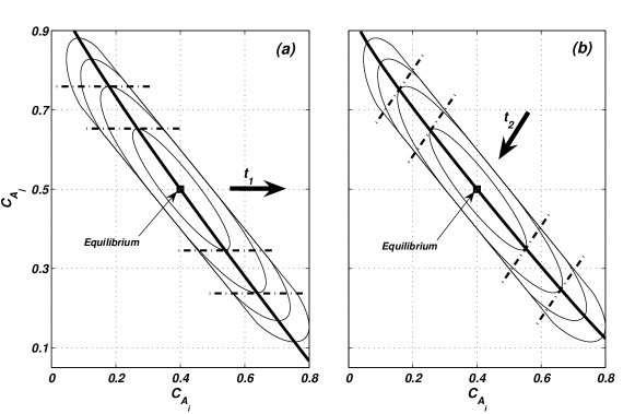
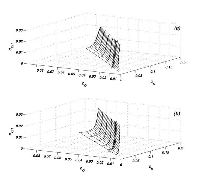
Figure 1: Quasi Equilibrium Manifold: the geometrical interpretation. Two different QE-manifolds (bold lines in (a) and (b)) corresponding to two different linear constraints subsets in the problem (23).

represents the QEM corresponding to the vector set {𝒎i}subscript𝒎𝑖\{\mbox{\boldmath$m$}_{i}\}. We want to stress the geometry behind (23) because it will be extensively exploited in the following. The geometric interpretation of a QEM is illustrated in Fig. 1 for a 222-dimensional phase-space (cAi,cAj)subscript𝑐subscript𝐴𝑖subscript𝑐subscript𝐴𝑗(c_{A_{i}},c_{A_{j}}). Let us consider the points where G𝐺G level curves (convex curves in Figures 1 (a)-(b)) are cut by the QE-manifolds (bold curves): in those points the inclination of the tangent to the G𝐺G-level curves is constant. Different QEM can be obtained by choosing different vector sets {𝒎i}subscript𝒎𝑖\{\mbox{\boldmath$m$}_{i}\}. A special choice is done when 𝒎1,,𝒎qsubscript𝒎1subscript𝒎𝑞\mbox{\boldmath$m$}_{1},...,\mbox{\boldmath$m$}_{q} are the q𝑞q left eigenvectors of the Jacobi matrix 𝑳(𝒄eq)𝑳superscript𝒄𝑒𝑞\mbox{\boldmath$L$}(\mbox{\boldmath$c$}^{eq}) corresponding to the q𝑞q smallest absolute eigenvalues. In that particular case, solution of (23) has its own name: Spectral Quasi Equilibrium Manifold (SQEM) [1, 2].

4.2 Quasi Equilibrium Manifold in practice

The minimization problem (23) can be, in principle, solved by the method of Lagrange multipliers. However, it is also well known that, when the number of constraints and variables increases, then that method becomes prohibitively complicated to implement. Since the number of species and elementary reaction steps is usually quite high, the Lagrange multipliers method is not suitable for most of the practical cases. For this reason, in the sequel a new procedure to overcome that issue is presented. An algorithm (Quasi Equilibrium Grid Algorithm-QEGA), which can be easily implemented in order to get a discrete analog of a QEM in any dimension, is developed. This is achieved by investigating further the QEM geometrical construction.

5 1D Quasi Equilibrium Grid (QEG) construction

Refer to caption
Figure 2: Quasi Equilibrium Grid: the basic idea.

Let us consider a one-dimensional quasi-equilibrium manifold. Let us assume that the node 𝒄0subscript𝒄0\mbox{\boldmath$c$}_{0} belongs to that manifold. One may now imagine to look for a new node 𝒄1subscript𝒄1\mbox{\boldmath$c$}_{1} which still lies on the quasi equilibrium manifold. In general, the node 𝒄1subscript𝒄1\mbox{\boldmath$c$}_{1} can be obtained from 𝒄0subscript𝒄0\mbox{\boldmath$c$}_{0} by adding a shift δ^𝒄0^𝛿subscript𝒄0\hat{\delta}\mbox{\boldmath$c$}_{0}: 𝒄1=𝒄0+δ^𝒄0subscript𝒄1subscript𝒄0^𝛿subscript𝒄0\mbox{\boldmath$c$}_{1}=\mbox{\boldmath$c$}_{0}+\hat{\delta}\mbox{\boldmath$c$}_{0}. That idea is applicable whenever a QEM-node 𝒄nsubscript𝒄𝑛\mbox{\boldmath$c$}_{n} is known and a new one 𝒄n+1subscript𝒄𝑛1\mbox{\boldmath$c$}_{n+1} must be found (see Fig. 2):

𝒄n+1=𝒄n+δ^𝒄n.subscript𝒄𝑛1subscript𝒄𝑛^𝛿subscript𝒄𝑛\mbox{\boldmath$c$}_{n+1}=\mbox{\boldmath$c$}_{n}+\hat{\delta}\mbox{\boldmath$c$}_{n}. (24)

First of all, any node 𝒄𝒄c has to fulfill the atom balances (6). Let {𝝆i}subscript𝝆𝑖\{\mbox{\boldmath$\rho$}_{i}\} be a basis in the null space of matrix 𝑫𝑫D. A convenient way to take automatically into account the conditions (6) is to express any shift δ^𝒄n^𝛿subscript𝒄𝑛\hat{\delta}\mbox{\boldmath$c$}_{n} as a linear combination of vectors 𝝆isubscript𝝆𝑖\mbox{\boldmath$\rho$}_{i}:

δ^𝒄n=i=1zμi𝝆i,^𝛿subscript𝒄𝑛superscriptsubscript𝑖1𝑧subscript𝜇𝑖subscript𝝆𝑖\hat{\delta}\mbox{\boldmath$c$}_{n}=\sum\nolimits_{i=1}^{z}{\mu_{i}\mbox{\boldmath$\rho$}_{i}}, (25)

where z=nl𝑧𝑛𝑙z=n-l is the dimension of the basis {𝝆i}subscript𝝆𝑖\{\mbox{\boldmath$\rho$}_{i}\}. By referring to Fig. 2, let us now discuss further the tangent space T𝑇T to the G𝐺G level surface in any quasi-equilibrium point 𝒄n+1subscript𝒄𝑛1\mbox{\boldmath$c$}_{n+1}. The space T𝑇T geometrically represents the linear constraint of the problem (23). Therefore, any point 𝒄𝒄c of T𝑇T satisfies that constraint, but only 𝒄n+1subscript𝒄𝑛1\mbox{\boldmath$c$}_{n+1} minimizes G𝐺G function. The line l𝑙\hbox to0.0pt{--\hss}l passing from 𝒄n+1subscript𝒄𝑛1\mbox{\boldmath$c$}_{n+1} and 𝒄𝒄c has the parametric form 𝒄=φ𝒕~+𝒄n+1𝒄𝜑bold-~𝒕subscript𝒄𝑛1\mbox{\boldmath$c$}=\varphi\mbox{\boldmath$\tilde{t}$}+\mbox{\boldmath$c$}_{n+1}, where 𝒕~bold-~𝒕\tilde{t} is a vector of T𝑇T spanning l𝑙\hbox to0.0pt{--\hss}l while φ𝜑\varphi is a parameter. In general, the linear constraints of the problem (23) can be also written as:

{(𝒎,𝒄)=φ(𝒎,𝒕~)+(𝒎,𝒄n+1)(𝒎,𝒕~)=0,𝒕~(𝒅i,𝒄)=φ(𝒅i,𝒕~)+(𝒅i,𝒄n+1)(𝒅i,𝒕~)=0,𝒕~cases𝒎𝒄𝜑𝒎bold-~𝒕𝒎subscript𝒄𝑛1𝒎bold-~𝒕0for-allbold-~𝒕missing-subexpressionmissing-subexpressionmissing-subexpressionmissing-subexpressionmissing-subexpressionmissing-subexpressionmissing-subexpressionmissing-subexpressionmissing-subexpressionmissing-subexpressionmissing-subexpressionmissing-subexpressionmissing-subexpressionmissing-subexpressionmissing-subexpressionmissing-subexpressionsubscript𝒅𝑖𝒄𝜑subscript𝒅𝑖bold-~𝒕subscript𝒅𝑖subscript𝒄𝑛1subscript𝒅𝑖bold-~𝒕0for-allbold-~𝒕missing-subexpressionmissing-subexpressionmissing-subexpressionmissing-subexpressionmissing-subexpressionmissing-subexpressionmissing-subexpressionmissing-subexpressionmissing-subexpressionmissing-subexpressionmissing-subexpressionmissing-subexpressionmissing-subexpressionmissing-subexpressionmissing-subexpressionmissing-subexpression\left\{\begin{array}[]{l}\begin{array}[]{*{20}c}{(\mbox{\boldmath$m$},\mbox{\boldmath$c$})=\varphi(\mbox{\boldmath$m$},\mbox{\boldmath$\tilde{t}$})+(\mbox{\boldmath$m$},\mbox{\boldmath$c$}_{n+1})}&\Rightarrow&{(\mbox{\boldmath$m$},\mbox{\boldmath$\tilde{t}$})=0,}&{\forall\mbox{\boldmath$\tilde{t}$}}\\ \end{array}\\ \begin{array}[]{*{20}c}{(\mbox{\boldmath$d$}_{i},\mbox{\boldmath$c$})=\varphi(\mbox{\boldmath$d$}_{i},\mbox{\boldmath$\tilde{t}$})+(\mbox{\boldmath$d$}_{i},\mbox{\boldmath$c$}_{n+1})}&\Rightarrow&{(\mbox{\boldmath$d$}_{i},\mbox{\boldmath$\tilde{t}$})=0,}&{\forall\mbox{\boldmath$\tilde{t}$}}\\ \end{array}\\ \end{array}\right. (26)

where 𝒎𝒎m and 𝒅isubscript𝒅𝑖\mbox{\boldmath$d$}_{i} are the reduced variable vector (q=1𝑞1q=1) and the generic row of matrix 𝑫𝑫D, respectively. The vector 𝒕~bold-~𝒕\tilde{t}, that respects (26), can always be written as a linear combination of some vectors 𝒕jsubscript𝒕𝑗\mbox{\boldmath$t$}_{j}, where {𝒕j}subscript𝒕𝑗\{\mbox{\boldmath$t$}_{j}\} denotes a basis in the null space of that matrix 𝑬𝑬E, whose first row is given by 𝒎𝒎m and the rest by the rows of 𝑫𝑫D:

𝑬=[𝒎𝑫].𝑬delimited-[]𝒎𝑫\mbox{\boldmath$E$}=\left[\begin{array}[]{l}\mbox{\boldmath$m$}\\ \mbox{\boldmath$D$}\\ \end{array}\right]. (27)

Note that the dimension of {𝒕j}subscript𝒕𝑗\{\mbox{\boldmath$t$}_{j}\} is z1𝑧1z-1. By looking at Fig. 2, the quasi-equilibrium requirement simply becomes the orthogonality condition:

(G(𝒄n+1),𝒕~)=0,𝒕~Tbold-∇𝐺subscript𝒄𝑛1bold-~𝒕0for-allbold-~𝒕𝑇missing-subexpressionmissing-subexpressionmissing-subexpressionmissing-subexpressionmissing-subexpressionmissing-subexpressionmissing-subexpressionmissing-subexpressionmissing-subexpressionmissing-subexpressionmissing-subexpressionmissing-subexpressionmissing-subexpressionmissing-subexpressionmissing-subexpressionmissing-subexpressionmissing-subexpressionmissing-subexpression\begin{array}[]{*{20}c}{(\mbox{\boldmath$\nabla$}G(\mbox{\boldmath$c$}_{n+1}),\mbox{\boldmath$\tilde{t}$})=0,}&{\forall\mbox{\boldmath$\tilde{t}$}\in T}\\ \end{array} (28)

which also means:

(G(𝒄n+1),𝒕j)=0,j=1,,z1.bold-∇𝐺subscript𝒄𝑛1subscript𝒕𝑗0for-all𝑗1𝑧1missing-subexpressionmissing-subexpressionmissing-subexpressionmissing-subexpressionmissing-subexpressionmissing-subexpressionmissing-subexpressionmissing-subexpressionmissing-subexpressionmissing-subexpressionmissing-subexpressionmissing-subexpressionmissing-subexpressionmissing-subexpressionmissing-subexpressionmissing-subexpressionmissing-subexpressionmissing-subexpression\begin{array}[]{*{20}c}{(\mbox{\boldmath$\nabla$}G(\mbox{\boldmath$c$}_{n+1}),\mbox{\boldmath$t$}_{j})=0,}&{\forall j=1,...,z-1}.\\ \end{array} (29)

The quasi-equilibrium grid algorithm is based on the equation system (29) and two more assumptions. First of all, we suppose that the known node 𝒄nsubscript𝒄𝑛\mbox{\boldmath$c$}_{n} is close to the QEM, although it does not necessarily belong to the QEM. Secondly, let the vector δ^𝒄n^𝛿subscript𝒄𝑛\hat{\delta}\mbox{\boldmath$c$}_{n} be small enough, so that the gradient G(𝒄n+1)bold-∇𝐺subscript𝒄𝑛1\mbox{\boldmath$\nabla$}G(\mbox{\boldmath$c$}_{n+1}) can be approximated to the first order:

G(𝒄n+1)G(𝒄n)+𝑯(𝒄n)δ^𝒄n,bold-∇𝐺subscript𝒄𝑛1bold-∇𝐺subscript𝒄𝑛𝑯subscript𝒄𝑛^𝛿subscript𝒄𝑛\mbox{\boldmath$\nabla$}G(\mbox{\boldmath$c$}_{n+1})\cong\mbox{\boldmath$\nabla$}G(\mbox{\boldmath$c$}_{n})+\mbox{\boldmath$H$}(\mbox{\boldmath$c$}_{n})\hat{\delta}\mbox{\boldmath$c$}_{n}, (30)

where 𝑯(𝒄n)=[2Gcicj]𝑯subscript𝒄𝑛delimited-[]superscript2𝐺subscript𝑐𝑖subscript𝑐𝑗\mbox{\boldmath$H$}(\mbox{\boldmath$c$}_{n})=\left[{\frac{{\partial^{2}G}}{{\partial c_{i}\partial c_{j}}}}\right] denotes again the matrix of second derivatives of the function G𝐺G evaluated at the point 𝒄nsubscript𝒄𝑛\mbox{\boldmath$c$}_{n}. By substituting equations (30) and (25) in (29), we obtain:

i=1z(𝒕j,𝑯(𝒄n)𝝆i)μi=(𝒕j,G(𝒄n)),j=1,,z1.superscriptsubscript𝑖1𝑧subscript𝒕𝑗𝑯subscript𝒄𝑛subscript𝝆𝑖subscript𝜇𝑖subscript𝒕𝑗bold-∇𝐺subscript𝒄𝑛for-all𝑗1𝑧1missing-subexpressionmissing-subexpressionmissing-subexpressionmissing-subexpressionmissing-subexpressionmissing-subexpressionmissing-subexpressionmissing-subexpressionmissing-subexpressionmissing-subexpressionmissing-subexpressionmissing-subexpressionmissing-subexpressionmissing-subexpressionmissing-subexpressionmissing-subexpressionmissing-subexpressionmissing-subexpression\begin{array}[]{*{20}c}{\sum\nolimits_{i=1}^{z}{(\mbox{\boldmath$t$}_{j},\mbox{\boldmath$H$}(\mbox{\boldmath$c$}_{n})\mbox{\boldmath$\rho$}_{i})}\mu_{i}=-(\mbox{\boldmath$t$}_{j},\mbox{\boldmath$\nabla$}G(\mbox{\boldmath$c$}_{n})),}&{\forall j=1,...,z-1}\\ \end{array}. (31)

By using the entropic scalar product (8), equations (31) can be cast into the form:

i=1z𝒕j,𝝆iμi=(𝒕j,G(𝒄n)),j=1,,z1.superscriptsubscript𝑖1𝑧subscript𝒕𝑗subscript𝝆𝑖subscript𝜇𝑖subscript𝒕𝑗bold-∇𝐺subscript𝒄𝑛for-all𝑗1𝑧1missing-subexpressionmissing-subexpressionmissing-subexpressionmissing-subexpressionmissing-subexpressionmissing-subexpressionmissing-subexpressionmissing-subexpressionmissing-subexpressionmissing-subexpressionmissing-subexpressionmissing-subexpressionmissing-subexpressionmissing-subexpressionmissing-subexpressionmissing-subexpressionmissing-subexpressionmissing-subexpression\begin{array}[]{*{20}c}{\sum\nolimits_{i=1}^{z}{\left\langle{\mbox{\boldmath$t$}_{j},\mbox{\boldmath$\rho$}_{i}}\right\rangle}\mu_{i}=-(\mbox{\boldmath$t$}_{j},\mbox{\boldmath$\nabla$}G(\mbox{\boldmath$c$}_{n})),}&{\forall j=1,...,z-1}\\ \end{array}. (32)

Both the matrix 𝑯𝑯H and the gradient Gbold-∇𝐺\mbox{\boldmath$\nabla$}G are calculated at the known node 𝒄nsubscript𝒄𝑛\mbox{\boldmath$c$}_{n}. Note that the right-hand side of (32) vanishes if the node 𝒄nsubscript𝒄𝑛\mbox{\boldmath$c$}_{n} belongs to the QEM. The node collection, subsequently evaluated through (32), will be called a Quasi Equilibrium Grid (QEG).

5.1 Closure through the spacing condition

Note, however, that the system (32) is not closed (z𝑧z unknowns μisubscript𝜇𝑖\mu_{i}, but z1𝑧1z-1 equations) because it lacks a further information about the grid spacing. A reasonable closure for that system can be achieved by fixing the grid spacing (e.g. in the Euclidean sense):

{i=1z𝒕j,𝝆iμi=(𝒕j,G(𝒄n)),j=1,,z1δ^𝒄n=εcasessuperscriptsubscript𝑖1𝑧subscript𝒕𝑗subscript𝝆𝑖subscript𝜇𝑖subscript𝒕𝑗bold-∇𝐺subscript𝒄𝑛for-all𝑗1𝑧1missing-subexpressionmissing-subexpressionmissing-subexpressionmissing-subexpressionmissing-subexpressionmissing-subexpressionmissing-subexpressionmissing-subexpressionmissing-subexpressionmissing-subexpressionmissing-subexpressionmissing-subexpressionmissing-subexpressionmissing-subexpressionmissing-subexpressionmissing-subexpressionmissing-subexpressionmissing-subexpressionnorm^𝛿subscript𝒄𝑛𝜀\left\{\begin{array}[]{l}\begin{array}[]{*{20}c}{\sum\nolimits_{i=1}^{z}{\left\langle{\mbox{\boldmath$t$}_{j},\mbox{\boldmath$\rho$}_{i}}\right\rangle}\mu_{i}=-(\mbox{\boldmath$t$}_{j},\mbox{\boldmath$\nabla$}G(\mbox{\boldmath$c$}_{n})),}&{\forall j=1,...,z-1}\\ \end{array}\\ \left\|{\hat{\delta}\mbox{\boldmath$c$}_{n}}\right\|=\varepsilon\\ \end{array}\right. (33)

where ε𝜀\varepsilon is a given number and δ^𝒄nnorm^𝛿subscript𝒄𝑛\left\|{\hat{\delta}\mbox{\boldmath$c$}_{n}}\right\| represents the Euclidean norm of the vector δ^𝒄n^𝛿subscript𝒄𝑛\hat{\delta}\mbox{\boldmath$c$}_{n}. The smaller ε𝜀\varepsilon is chosen, the more accurate the expression (30) gets. As it will be shown later on, for small ε𝜀\varepsilon the Quasi Equilibrium Grid lies very close to the correspondent Quasi Equilibrium Manifold. The extra condition makes (33) a non-linear algebraic system. A way to solve it will be now discussed. The idea is to find the general solution of the linear system (32), and then to choose the one which also fulfills the non linear condition in (33). Let the basis {𝝆i}subscript𝝆𝑖\{\mbox{\boldmath$\rho$}_{i}\} be orthonormal (in the Euclidean sense). That is not crucial, but it proves to be convenient in the following analysis; indeed the non-linear system (33) now is cast as follows:

{i=1z𝒕j,𝝆iμi=(𝒕j,G(𝒄n)),j=1,,z1i=1zμi2=ε2.casessuperscriptsubscript𝑖1𝑧subscript𝒕𝑗subscript𝝆𝑖subscript𝜇𝑖subscript𝒕𝑗bold-∇𝐺subscript𝒄𝑛for-all𝑗1𝑧1missing-subexpressionmissing-subexpressionmissing-subexpressionmissing-subexpressionmissing-subexpressionmissing-subexpressionmissing-subexpressionmissing-subexpressionmissing-subexpressionmissing-subexpressionmissing-subexpressionmissing-subexpressionmissing-subexpressionmissing-subexpressionmissing-subexpressionmissing-subexpressionmissing-subexpressionmissing-subexpressionsuperscriptsubscript𝑖1𝑧superscriptsubscript𝜇𝑖2superscript𝜀2\left\{\begin{array}[]{l}\begin{array}[]{*{20}c}{\sum\nolimits_{i=1}^{z}{\left\langle{\mbox{\boldmath$t$}_{j},\mbox{\boldmath$\rho$}_{i}}\right\rangle}\mu_{i}=-(\mbox{\boldmath$t$}_{j},\mbox{\boldmath$\nabla$}G(\mbox{\boldmath$c$}_{n})),}&{\forall j=1,...,z-1}\\ \end{array}\\ \sum\nolimits_{i=1}^{z}{\mu_{i}^{2}}=\varepsilon^{2}.\\ \end{array}\right. (34)

The general solution of (32) can always be written as:

[μ1μz]=w[ν1νz]+[p1pz],delimited-[]subscript𝜇1missing-subexpressionmissing-subexpressionmissing-subexpressionmissing-subexpressionmissing-subexpressionmissing-subexpressionmissing-subexpressionmissing-subexpressionmissing-subexpressionmissing-subexpressionmissing-subexpressionmissing-subexpressionmissing-subexpressionmissing-subexpressionmissing-subexpressionmissing-subexpressionmissing-subexpressionmissing-subexpressionmissing-subexpressionmissing-subexpressionmissing-subexpressionmissing-subexpressionmissing-subexpressionmissing-subexpressionmissing-subexpressionmissing-subexpressionmissing-subexpressionmissing-subexpressionmissing-subexpressionmissing-subexpressionmissing-subexpressionmissing-subexpressionmissing-subexpressionmissing-subexpressionmissing-subexpressionmissing-subexpressionmissing-subexpressionmissing-subexpressionsubscript𝜇𝑧missing-subexpressionmissing-subexpressionmissing-subexpressionmissing-subexpressionmissing-subexpressionmissing-subexpressionmissing-subexpressionmissing-subexpressionmissing-subexpressionmissing-subexpressionmissing-subexpressionmissing-subexpressionmissing-subexpressionmissing-subexpressionmissing-subexpressionmissing-subexpressionmissing-subexpressionmissing-subexpressionmissing-subexpression𝑤delimited-[]subscript𝜈1missing-subexpressionmissing-subexpressionmissing-subexpressionmissing-subexpressionmissing-subexpressionmissing-subexpressionmissing-subexpressionmissing-subexpressionmissing-subexpressionmissing-subexpressionmissing-subexpressionmissing-subexpressionmissing-subexpressionmissing-subexpressionmissing-subexpressionmissing-subexpressionmissing-subexpressionmissing-subexpressionmissing-subexpressionmissing-subexpressionmissing-subexpressionmissing-subexpressionmissing-subexpressionmissing-subexpressionmissing-subexpressionmissing-subexpressionmissing-subexpressionmissing-subexpressionmissing-subexpressionmissing-subexpressionmissing-subexpressionmissing-subexpressionmissing-subexpressionmissing-subexpressionmissing-subexpressionmissing-subexpressionmissing-subexpressionmissing-subexpressionsubscript𝜈𝑧missing-subexpressionmissing-subexpressionmissing-subexpressionmissing-subexpressionmissing-subexpressionmissing-subexpressionmissing-subexpressionmissing-subexpressionmissing-subexpressionmissing-subexpressionmissing-subexpressionmissing-subexpressionmissing-subexpressionmissing-subexpressionmissing-subexpressionmissing-subexpressionmissing-subexpressionmissing-subexpressionmissing-subexpressiondelimited-[]subscript𝑝1missing-subexpressionmissing-subexpressionmissing-subexpressionmissing-subexpressionmissing-subexpressionmissing-subexpressionmissing-subexpressionmissing-subexpressionmissing-subexpressionmissing-subexpressionmissing-subexpressionmissing-subexpressionmissing-subexpressionmissing-subexpressionmissing-subexpressionmissing-subexpressionmissing-subexpressionmissing-subexpressionmissing-subexpressionmissing-subexpressionmissing-subexpressionmissing-subexpressionmissing-subexpressionmissing-subexpressionmissing-subexpressionmissing-subexpressionmissing-subexpressionmissing-subexpressionmissing-subexpressionmissing-subexpressionmissing-subexpressionmissing-subexpressionmissing-subexpressionmissing-subexpressionmissing-subexpressionmissing-subexpressionmissing-subexpressionmissing-subexpressionsubscript𝑝𝑧missing-subexpressionmissing-subexpressionmissing-subexpressionmissing-subexpressionmissing-subexpressionmissing-subexpressionmissing-subexpressionmissing-subexpressionmissing-subexpressionmissing-subexpressionmissing-subexpressionmissing-subexpressionmissing-subexpressionmissing-subexpressionmissing-subexpressionmissing-subexpressionmissing-subexpressionmissing-subexpressionmissing-subexpression\left[{\begin{array}[]{*{20}c}{\mu_{1}}\\ {\vdots}\\ {\mu_{z}}\\ \end{array}}\right]=w\left[{\begin{array}[]{*{20}c}{\nu_{1}}\\ {\vdots}\\ {\nu_{z}}\\ \end{array}}\right]+\left[{\begin{array}[]{*{20}c}{p_{1}}\\ {\vdots}\\ {p_{z}}\\ \end{array}}\right], (35)

where w𝑤w is a free parameter, while 𝝂=[ν1,,νz]T𝝂superscriptsubscript𝜈1subscript𝜈𝑧𝑇\mbox{\boldmath$\nu$}=[\nu_{1},...,\nu_{z}]^{T} and 𝒑=[p1,,pz]T𝒑superscriptsubscript𝑝1subscript𝑝𝑧𝑇\mbox{\boldmath$p$}=[p_{1},...,p_{z}]^{T} are the solution of the homogeneous problem and a special solution of (32), respectively. Without any restriction, we assume (𝝂,𝝂)=1𝝂𝝂1(\mbox{\boldmath$\nu$},\mbox{\boldmath$\nu$})=1. Once 𝝂𝝂\nu and 𝒑𝒑p are known, the non linear equation of (34) can be written, in terms of w𝑤w, as:

w2+2(𝝂,𝒑)w+(𝒑,𝒑)ε2=0.superscript𝑤22𝝂𝒑𝑤𝒑𝒑superscript𝜀20w^{2}+2(\mbox{\boldmath$\nu$},\mbox{\boldmath$p$})w+(\mbox{\boldmath$p$},\mbox{\boldmath$p$})-\varepsilon^{2}=0. (36)

If the solvability condition is satisfied,

(𝝂,𝒑)2(𝒑,𝒑)+ε2>0,superscript𝝂𝒑2𝒑𝒑superscript𝜀20\left({\mbox{\boldmath$\nu$},\mbox{\boldmath$p$}}\right)^{2}-(\mbox{\boldmath$p$},\mbox{\boldmath$p$})+\varepsilon^{2}>0, (37)

then the two real valued solutions of (36) (wIsuperscript𝑤𝐼w^{I}, wIIsuperscript𝑤𝐼𝐼w^{II}), upon substitution into (35), give two possible sets [μ1,,μz]subscript𝜇1subscript𝜇𝑧[\mu_{1},...,\mu_{z}]. Therefore, by using the (24) and (25), two new nodes 𝒄n+1I,𝒄n+1IIsuperscriptsubscript𝒄𝑛1𝐼superscriptsubscript𝒄𝑛1𝐼𝐼\mbox{\boldmath$c$}_{n+1}^{I},\mbox{\boldmath$c$}_{n+1}^{II} (both close to the quasi equilibrium curve) can be evaluated from the previous one 𝒄nsubscript𝒄𝑛\mbox{\boldmath$c$}_{n} (see Fig. 3).

Refer to caption
Figure 3: Two solutions for the 1D QEG algorithm.

A criterion, able to choose between those two solutions, depends on the phase-space zone where the grid needs to be constructed. This idea will be clarified in the following example. Usually, the equilibrium point is supposed to be a good starting node for the QEG procedure: 𝒄0=𝒄eqsubscript𝒄0superscript𝒄𝑒𝑞\mbox{\boldmath$c$}_{0}=\mbox{\boldmath$c$}^{eq}.

Remark. The QEG-equations (32) can be generalized as follows:

i=1z𝒕j,𝝆iμi=η(𝒕j,G(𝒄n)),j=1,,z1,superscriptsubscript𝑖1𝑧subscript𝒕𝑗subscript𝝆𝑖subscript𝜇𝑖𝜂subscript𝒕𝑗bold-∇𝐺subscript𝒄𝑛for-all𝑗1𝑧1missing-subexpressionmissing-subexpressionmissing-subexpressionmissing-subexpressionmissing-subexpressionmissing-subexpressionmissing-subexpressionmissing-subexpressionmissing-subexpressionmissing-subexpressionmissing-subexpressionmissing-subexpressionmissing-subexpressionmissing-subexpressionmissing-subexpressionmissing-subexpressionmissing-subexpressionmissing-subexpression\begin{array}[]{*{20}c}{\sum\nolimits_{i=1}^{z}{\left\langle{\mbox{\boldmath$t$}_{j},\mbox{\boldmath$\rho$}_{i}}\right\rangle}\mu_{i}=-\eta(\mbox{\boldmath$t$}_{j},\mbox{\boldmath$\nabla$}G(\mbox{\boldmath$c$}_{n})),}&{\forall j=1,...,z-1},\\ \end{array} (38)

where η𝜂\eta is a parameter 0η10𝜂10\leq\eta\leq 1. When η=1𝜂1\eta=1, (32) is recovered. On the other hand, if the QEG-nodes are close to the QEM, then the non-homogeneous terms can be neglected (they vanish on the QEM). Therefore, a reasonable approximation of the system (32) is given when η=0𝜂0\eta=0. In the latter case, the solvability condition (37) is fulfilled. If η=1𝜂1\eta=1 and (37) does not hold, that parameter can be chosen in such a way that the solvability condition is satisfied. In the example below, solvability condition (37) is always satisfied and we use (33).

6 1D SQEG algorithm at work

In this section, an example will be considered in order to illustrate how the algorithm, described in the previous section, works for finding a one-dimensional SQE-grid. That grid will be compared with the relative spectral quasi-equilibrium manifold, too. Let us consider the following four-step three-component reaction (kindly suggested by A.N. Gorban):

{1.AB,k1+=1,2.BC,k2+=1,3.CA,k3+=1,4.A+B2C,k4+=50.\left\{\begin{array}[]{l}1.A\leftrightarrow B,\quad k_{1}^{+}=1,\\ 2.B\leftrightarrow C,\quad k_{2}^{+}=1,\\ 3.C\leftrightarrow A,\quad k_{3}^{+}=1,\\ 4.A+B\leftrightarrow 2C,\quad k_{4}^{+}=50.\\ \end{array}\right. (39)

The atom balance takes the form:

𝑫𝒄=[111][cAcBcC]=1,𝑫𝒄delimited-[]111missing-subexpressionmissing-subexpressionmissing-subexpressionmissing-subexpressionmissing-subexpressionmissing-subexpressionmissing-subexpressionmissing-subexpressionmissing-subexpressionmissing-subexpressionmissing-subexpressionmissing-subexpressionmissing-subexpressionmissing-subexpressionmissing-subexpressionmissing-subexpressionmissing-subexpressiondelimited-[]subscript𝑐𝐴missing-subexpressionmissing-subexpressionmissing-subexpressionmissing-subexpressionmissing-subexpressionmissing-subexpressionmissing-subexpressionmissing-subexpressionmissing-subexpressionmissing-subexpressionmissing-subexpressionmissing-subexpressionmissing-subexpressionmissing-subexpressionmissing-subexpressionmissing-subexpressionmissing-subexpressionmissing-subexpressionmissing-subexpressionsubscript𝑐𝐵missing-subexpressionmissing-subexpressionmissing-subexpressionmissing-subexpressionmissing-subexpressionmissing-subexpressionmissing-subexpressionmissing-subexpressionmissing-subexpressionmissing-subexpressionmissing-subexpressionmissing-subexpressionmissing-subexpressionmissing-subexpressionmissing-subexpressionmissing-subexpressionmissing-subexpressionmissing-subexpressionmissing-subexpressionsubscript𝑐𝐶missing-subexpressionmissing-subexpressionmissing-subexpressionmissing-subexpressionmissing-subexpressionmissing-subexpressionmissing-subexpressionmissing-subexpressionmissing-subexpressionmissing-subexpressionmissing-subexpressionmissing-subexpressionmissing-subexpressionmissing-subexpressionmissing-subexpressionmissing-subexpressionmissing-subexpressionmissing-subexpressionmissing-subexpression1\mbox{\boldmath$D$}\mbox{\boldmath$c$}=\left[{\begin{array}[]{*{20}c}1&1&1\\ \end{array}}\right]\left[{\begin{array}[]{*{20}c}{c_{A}}\\ {c_{B}}\\ {c_{C}}\\ \end{array}}\right]=1, (40)

and the equilibrium point is chosen as: cAeq=0.1superscriptsubscript𝑐𝐴𝑒𝑞0.1c_{A}^{eq}=0.1, cBeq=0.5superscriptsubscript𝑐𝐵𝑒𝑞0.5c_{B}^{eq}=0.5, cCeq=0.4superscriptsubscript𝑐𝐶𝑒𝑞0.4c_{C}^{eq}=0.4.

Refer to caption
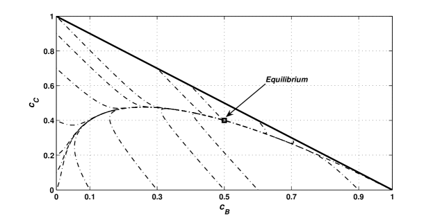
Figure 4: Reaction (39): some trajectories projected into the phase-subspace (cC,cB)subscript𝑐𝐶subscript𝑐𝐵(c_{C},c_{B}).

As Fig. 4 shows, the system is effectively two-dimensional, so the quasi-equilibrium manifold is expected to provide an one-dimensional reduced description (q=1𝑞1q=1). Indeed, any solution trajectory, after a rapid initial dynamics, is attracted to a 1D curve and along it reaches the equilibrium point. If the system is closed and the reaction (39) takes place under constant volume and temperature, we can assume that the system is supported by the Lyapunov function G𝐺G (7):

G=cA[ln(cAcAeq)1]+cB[ln(cBcBeq)1]+cC[ln(cCcCeq)1].𝐺subscript𝑐𝐴delimited-[]subscript𝑐𝐴superscriptsubscript𝑐𝐴𝑒𝑞1subscript𝑐𝐵delimited-[]subscript𝑐𝐵superscriptsubscript𝑐𝐵𝑒𝑞1subscript𝑐𝐶delimited-[]subscript𝑐𝐶superscriptsubscript𝑐𝐶𝑒𝑞1G=c_{A}\left[{\ln\left({\frac{{c_{A}}}{{c_{A}^{eq}}}}\right)-1}\right]+c_{B}\left[{\ln\left({\frac{{c_{B}}}{{c_{B}^{eq}}}}\right)-1}\right]+c_{C}\left[{\ln\left({\frac{{c_{C}}}{{c_{C}^{eq}}}}\right)-1}\right]. (41)

Once a 3-dimensional vector 𝒎𝒎m has been chosen, the QEM equation can be found by solving the variational problem (23):

{Gmin(𝒎,𝒄)=ξ𝑫𝒄=1.cases𝐺𝒎𝒄𝜉𝑫𝒄1\left\{\begin{array}[]{l}G\to\min\\ (\mbox{\boldmath$m$},\mbox{\boldmath$c$})=\xi\\ \mbox{\boldmath$D$}\mbox{\boldmath$c$}=1.\\ \end{array}\right. (42)

In the following, the Spectral Quasi Equilibrium Manifold (SQEM) [2, 1] will be constructed. The Jacobian matrix 𝑳𝑳L in the equilibrium point and its slowest left eigenvector 𝒙lssuperscriptsubscript𝒙𝑙𝑠\mbox{\boldmath$x$}_{l}^{s} are:

𝑳(𝒄eq)=[304.813.5246.213.75541127.25],𝒙ls=[0.8807,0.3905,0.2681].𝑳superscript𝒄𝑒𝑞delimited-[]304.813.5missing-subexpressionmissing-subexpressionmissing-subexpressionmissing-subexpressionmissing-subexpressionmissing-subexpressionmissing-subexpressionmissing-subexpressionmissing-subexpressionmissing-subexpressionmissing-subexpressionmissing-subexpressionmissing-subexpressionmissing-subexpressionmissing-subexpressionmissing-subexpressionmissing-subexpression246.213.75missing-subexpressionmissing-subexpressionmissing-subexpressionmissing-subexpressionmissing-subexpressionmissing-subexpressionmissing-subexpressionmissing-subexpressionmissing-subexpressionmissing-subexpressionmissing-subexpressionmissing-subexpressionmissing-subexpressionmissing-subexpressionmissing-subexpressionmissing-subexpressionmissing-subexpression541127.25missing-subexpressionmissing-subexpressionmissing-subexpressionmissing-subexpressionmissing-subexpressionmissing-subexpressionmissing-subexpressionmissing-subexpressionmissing-subexpressionmissing-subexpressionmissing-subexpressionmissing-subexpressionmissing-subexpressionmissing-subexpressionmissing-subexpressionmissing-subexpressionmissing-subexpressionmissing-subexpressionsuperscriptsubscript𝒙𝑙𝑠delimited-[]0.88070.39050.2681missing-subexpressionmissing-subexpressionmissing-subexpressionmissing-subexpressionmissing-subexpressionmissing-subexpressionmissing-subexpressionmissing-subexpressionmissing-subexpressionmissing-subexpressionmissing-subexpressionmissing-subexpressionmissing-subexpressionmissing-subexpressionmissing-subexpressionmissing-subexpressionmissing-subexpressionmissing-subexpressionmissing-subexpressionmissing-subexpressionmissing-subexpressionmissing-subexpressionmissing-subexpressionmissing-subexpressionmissing-subexpressionmissing-subexpressionmissing-subexpressionmissing-subexpressionmissing-subexpressionmissing-subexpressionmissing-subexpressionmissing-subexpressionmissing-subexpressionmissing-subexpression\begin{array}[]{*{20}c}{\mbox{\boldmath$L$}(\mbox{\boldmath$c$}^{eq})=\left[{\begin{array}[]{*{20}c}{-30}&{-4.8}&{13.5}\\ {-24}&{-6.2}&{13.75}\\ {54}&{11}&{-27.25}\\ \end{array}}\right],}&{}\hfil&{\mbox{\boldmath$x$}_{l}^{s}=\left[{\begin{array}[]{*{20}c}{0.8807,}&{-0.3905,}&{0.2681}\\ \end{array}}\right]}.\\ \end{array} (43)

Solution of the problem (42), with the choice 𝒎=𝒙ls𝒎superscriptsubscript𝒙𝑙𝑠\mbox{\boldmath$m$}=\mbox{\boldmath$x$}_{l}^{s}, delivers the 1D SQEM for the case shown in Fig 4. To this end, let us rewrite the (42) in a more explicit form:

{c0A=0.3072+0.7867ξ0.5180ϕ(ξ)c0B=0.69280.7867ξ0.4820ϕ(ξ)c0C=ϕ(ξ)G(ϕ,ξ)ϕ=0,2G(ϕ,ξ)ϕ2>0,casessubscript𝑐0𝐴0.30720.7867𝜉0.5180italic-ϕ𝜉subscript𝑐0𝐵0.69280.7867𝜉0.4820italic-ϕ𝜉subscript𝑐0𝐶italic-ϕ𝜉𝐺italic-ϕ𝜉italic-ϕ0missing-subexpressionsuperscript2𝐺italic-ϕ𝜉superscriptitalic-ϕ20missing-subexpressionmissing-subexpressionmissing-subexpressionmissing-subexpressionmissing-subexpressionmissing-subexpressionmissing-subexpressionmissing-subexpressionmissing-subexpressionmissing-subexpressionmissing-subexpressionmissing-subexpressionmissing-subexpressionmissing-subexpressionmissing-subexpressionmissing-subexpressionmissing-subexpression\left\{\begin{array}[]{l}c_{0A}=0.3072+0.7867\xi-0.5180\phi(\xi)\\ c_{0B}=0.6928-0.7867\xi-0.4820\phi(\xi)\\ c_{0C}=\phi(\xi)\\ \begin{array}[]{*{20}c}{\frac{{\partial G(\phi,\xi)}}{{\partial\phi}}=0,}&{}\hfil&{\frac{{\partial^{2}G(\phi,\xi)}}{{\partial\phi^{2}}}>0,}\\ \end{array}\\ \end{array}\right. (44)

where 𝒄0=[c0A,c0B,c0C]subscript𝒄0subscript𝑐0𝐴subscript𝑐0𝐵subscript𝑐0𝐶\mbox{\boldmath$c$}_{0}=[c_{0A},c_{0B},c_{0C}] is the solution of the problem (42), while ϕitalic-ϕ\phi denotes the relation between cCsubscript𝑐𝐶c_{C} and the reduced variable ξ𝜉\xi on the SQEM. By using the G𝐺G function (41), the problem (44) is equivalent to the implicit equation

(0.3072+0.7867ξ0.5180ϕ0.1)0.5180(0.69280.7867ξ0.4820ϕ0.5)0.4820(ϕ0.4)1=0.superscript0.30720.7867𝜉0.5180italic-ϕ0.10.5180superscript0.69280.7867𝜉0.4820italic-ϕ0.50.4820italic-ϕ0.410\left({\frac{{0.3072+0.7867\xi-0.5180\phi}}{{0.1}}}\right)^{-0.5180}\left({\frac{{0.6928-0.7867\xi-0.4820\phi}}{{0.5}}}\right)^{-0.4820}\left({\frac{\phi}{{0.4}}}\right)-1=0. (45)

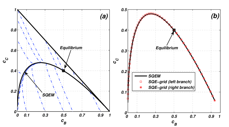
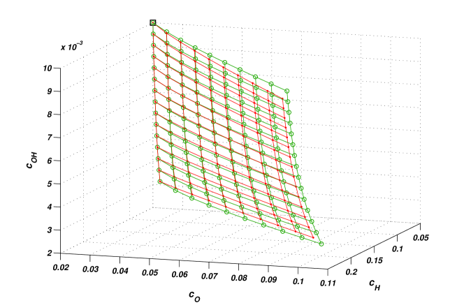
The solution of (45), by means of relations (44), gives the SQEM shown in Fig. 5(a). One may now apply the QEG-algorithm described above, in order to make a comparison with the analytic solution just found. An orthonormal basis {𝝆i}subscript𝝆𝑖\{\mbox{\boldmath$\rho$}_{i}\} in the null space of the matrix 𝑫=[111]𝑫delimited-[]111missing-subexpressionmissing-subexpressionmissing-subexpressionmissing-subexpressionmissing-subexpressionmissing-subexpressionmissing-subexpressionmissing-subexpressionmissing-subexpressionmissing-subexpressionmissing-subexpressionmissing-subexpressionmissing-subexpressionmissing-subexpressionmissing-subexpressionmissing-subexpressionmissing-subexpression\mbox{\boldmath$D$}=\left[{\begin{array}[]{*{20}c}1&1&1\\ \end{array}}\right] has dimension z=2𝑧2z=2 and can be chosen as follows:

{𝝆1=[0.5774,0.7887,0.2113],𝝆2=[0.5774,0.2113,0.7887].casessubscript𝝆10.57740.78870.2113subscript𝝆20.57740.21130.7887\left\{\begin{array}[]{l}\mbox{\boldmath$\rho$}_{1}=[-0.5774,0.7887,-0.2113],\\ \mbox{\boldmath$\rho$}_{2}=[-0.5774,-0.2113,0.7887].\\ \end{array}\right. (46)

Since the matrix 𝑬𝑬E has the form:

𝑬=[0.88070.39050.2680111],𝑬delimited-[]0.88070.39050.2680missing-subexpressionmissing-subexpressionmissing-subexpressionmissing-subexpressionmissing-subexpressionmissing-subexpressionmissing-subexpressionmissing-subexpressionmissing-subexpressionmissing-subexpressionmissing-subexpressionmissing-subexpressionmissing-subexpressionmissing-subexpressionmissing-subexpressionmissing-subexpressionmissing-subexpression111missing-subexpressionmissing-subexpressionmissing-subexpressionmissing-subexpressionmissing-subexpressionmissing-subexpressionmissing-subexpressionmissing-subexpressionmissing-subexpressionmissing-subexpressionmissing-subexpressionmissing-subexpressionmissing-subexpressionmissing-subexpressionmissing-subexpressionmissing-subexpressionmissing-subexpression\mbox{\boldmath$E$}=\left[{\begin{array}[]{*{20}c}{0.8807}&{-0.3905}&{0.2680}\\ 1&1&1\\ \end{array}}\right], (47)

a vector 𝒕𝒕t spanning ker(𝑬(\mbox{\boldmath$E$}) is:

𝒕=[0.4229,0.3934,0.8163].𝒕0.42290.39340.8163\mbox{\boldmath$t$}=[-0.4229,-0.3934,0.8163].

The system (34), in this example, simply reads:

{𝒕,𝝆1μ1+𝒕,𝝆2μ2=(𝒕,G)μ12+μ22=ε2.cases𝒕subscript𝝆1subscript𝜇1𝒕subscript𝝆2subscript𝜇2𝒕bold-∇𝐺superscriptsubscript𝜇12superscriptsubscript𝜇22superscript𝜀2\left\{\begin{array}[]{l}\left\langle{\mbox{\boldmath$t$},\mbox{\boldmath$\rho$}_{1}}\right\rangle\mu_{1}+\left\langle{\mbox{\boldmath$t$},\mbox{\boldmath$\rho$}_{2}}\right\rangle\mu_{2}=-\left({\mbox{\boldmath$t$},\mbox{\boldmath$\nabla$}G}\right)\\ \mu_{1}^{2}+\mu_{2}^{2}=\varepsilon^{2}.\\ \end{array}\right. (48)

By solving (48) in a QEG-node 𝒄nsubscript𝒄𝑛\mbox{\boldmath$c$}_{n}, the shift vector δ^𝒄n=μ1𝝆1+μ2𝝆2^𝛿subscript𝒄𝑛subscript𝜇1subscript𝝆1subscript𝜇2subscript𝝆2\hat{\delta}\mbox{\boldmath$c$}_{n}=\mu_{1}\mbox{\boldmath$\rho$}_{1}+\mu_{2}\mbox{\boldmath$\rho$}_{2} allows to evaluate the new QEG-node 𝒄n+1=𝒄n+δ^𝒄nsubscript𝒄𝑛1subscript𝒄𝑛^𝛿subscript𝒄𝑛\mbox{\boldmath$c$}_{n+1}=\mbox{\boldmath$c$}_{n}+\hat{\delta}\mbox{\boldmath$c$}_{n}. The QEG procedure, starting from the equilibrium point 𝒄eq=𝒄0superscript𝒄𝑒𝑞subscript𝒄0\mbox{\boldmath$c$}^{eq}=\mbox{\boldmath$c$}_{0}, was performed twice, keeping uniformly parameter ε2=103superscript𝜀2superscript103\varepsilon^{2}=10^{-3}. The first time, by choosing the solution in such a way that cBn+1<cBnsubscript𝑐subscript𝐵𝑛1subscript𝑐subscript𝐵𝑛c_{B_{n+1}}<c_{B_{n}}, the left branch of the SQE-grid was obtained; then, by imposing cBn+1>cBnsubscript𝑐subscript𝐵𝑛1subscript𝑐subscript𝐵𝑛c_{B_{n+1}}>c_{B_{n}}, also the right branch was calculated. The algorithm was terminated as soon as at least one component of the new node 𝒄n+1subscript𝒄𝑛1\mbox{\boldmath$c$}_{n+1} becomes negative.

Refer to caption
Figure 5: (a) The bold curve is the SQE-manifold which was analytically evaluated by solving the (45). In that case the SQEM represents a very good approximation of the invariant manifold. (b) The SQE-manifold is compared with the SQE-grid where ε2=103superscript𝜀2superscript103\varepsilon^{2}=10^{-3}.

The result, shown in Fig. 5(b), proves that the SQE-grid is in excellent agreement with the analytical curve (SQEM).

6.1 Grid spacing choice
Refer to caption
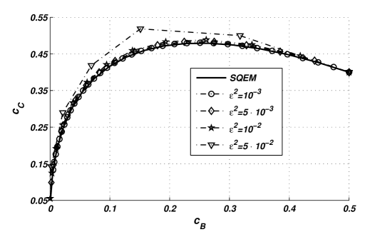
Figure 6: SQEG Left branch of the case in Fig. 5 (b). Different approximations compared with the analytical solution (SQEM). Each grid is calculated by using a different parameter ε𝜀\varepsilon.

There is no need to stress the importance of the grid spacing parameter ε𝜀\varepsilon for the QEG accuracy. In the case of Section 6, the SQEG was computed several times with different values of ε𝜀\varepsilon. The QEG algorithm is based on the linear approximation (30). Therefore, the smaller is δ^𝒄n=εnorm^𝛿subscript𝒄𝑛𝜀\left\|{\hat{\delta}\mbox{\boldmath$c$}_{n}}\right\|=\varepsilon the more accurate is the QEM description by means of the QEG. Nevertheless, the smaller is ε𝜀\varepsilon the larger is the number of times that the system (33) must be solved to have a grid of a fixed size. For this reason, we need to keep ε𝜀\varepsilon as large as possible. We estimated (at least the order of magnitude) the upper limit of spacing (εusubscript𝜀𝑢\varepsilon_{u}) which gives a QEG “not far” from the relative QEM. From our numerical experiments, a reasonable value for that was εu101subscript𝜀𝑢superscript101\varepsilon_{u}\cong 10^{-1}. As Fig. 6 shows, the QEG is not far from the QEM even for a quite coarse grid (ε>εu𝜀subscript𝜀𝑢\varepsilon>\varepsilon_{u}).

7 Generalization to multi-dimensional grids

The QEG algorithm, which has been developed for constructing 111-dimensional grids, can be modified in order to get multi-dimensional grids, whenever needed. From all reasonable extension strategies, two of them here will be analyzed: a straightforward extension and a flag extension (flag extension, for invariant grids, was introduced in Ref. [3]). In the first case, the algorithm of paragraph 5 and the equation system (34) are tuned for a q𝑞q-dimensional grid calculation. Here, the implicit assumption is that the grid dimension q𝑞q is fixed and uniform everywhere in the phase space (like for the QEM construction). However, a second flexible approach, suitable for SQEG construction, was developed, too. In that case, the grid dimension can be varied at will.

7.1 The straightforward extension

According to the straightforward extension, if a node 𝒄nsubscript𝒄𝑛\mbox{\boldmath$c$}_{n} close to the q𝑞q-dimensional QEM is known, then a new node 𝒄n+1subscript𝒄𝑛1\mbox{\boldmath$c$}_{n+1} can be added to the QE-grid by shifting 𝒄nsubscript𝒄𝑛\mbox{\boldmath$c$}_{n}:

𝒄n+1=𝒄n+δ^𝒄n,δ^𝒄n=i=1zμi𝝆i,formulae-sequencesubscript𝒄𝑛1subscript𝒄𝑛^𝛿subscript𝒄𝑛^𝛿subscript𝒄𝑛superscriptsubscript𝑖1𝑧subscript𝜇𝑖subscript𝝆𝑖\mbox{\boldmath$c$}_{n+1}=\mbox{\boldmath$c$}_{n}+\hat{\delta}\mbox{\boldmath$c$}_{n},\quad\hat{\delta}\mbox{\boldmath$c$}_{n}=\sum\nolimits_{i=1}^{z}{\mu_{i}\mbox{\boldmath$\rho$}_{i}}, (49)

where {𝝆i}subscript𝝆𝑖\{\mbox{\boldmath$\rho$}_{i}\} is still a basis in the null space of matrix 𝑫𝑫D. The linear constraints of the problem (23) define the tangent space T𝑇T to the G𝐺G level surfaces in the new node 𝒄n+1subscript𝒄𝑛1\mbox{\boldmath$c$}_{n+1}. Let 𝒄𝒄c be a generic point of T𝑇T, the line l𝑙\hbox to0.0pt{--\hss}l passing from 𝒄n+1subscript𝒄𝑛1\mbox{\boldmath$c$}_{n+1} and 𝒄𝒄c has the parametric form: 𝒄=φ𝒕~+𝒄n+1𝒄𝜑bold-~𝒕subscript𝒄𝑛1\mbox{\boldmath$c$}=\varphi\mbox{\boldmath$\tilde{t}$}+\mbox{\boldmath$c$}_{n+1}, where 𝒕~bold-~𝒕\tilde{t} is the vector of T𝑇T which spans l𝑙\hbox to0.0pt{--\hss}l and φ𝜑\varphi is the parameter. The generalized form of the relations (26) is:

{(𝒎1,𝒄)=φ(𝒎1,𝒕~)+(𝒎1,𝒄n+1i)(𝒎1,𝒕~)=0,𝒕~T(𝒎q,𝒄)=φ(𝒎q,𝒕~)+(𝒎q,𝒄n+1i)(𝒎q,𝒕~)=0,𝒕~T(𝒅i,𝒄)=φ(𝒅i,𝒕~)+(𝒅i,𝒄n+1i)(𝒅i,𝒕~)=0,𝒕~T,casesformulae-sequencesubscript𝒎1𝒄𝜑subscript𝒎1bold-~𝒕subscript𝒎1superscriptsubscript𝒄𝑛1𝑖subscript𝒎1bold-~𝒕0for-allbold-~𝒕𝑇formulae-sequencesubscript𝒎𝑞𝒄𝜑subscript𝒎𝑞bold-~𝒕subscript𝒎𝑞superscriptsubscript𝒄𝑛1𝑖subscript𝒎𝑞bold-~𝒕0for-allbold-~𝒕𝑇formulae-sequencesubscript𝒅𝑖𝒄𝜑subscript𝒅𝑖bold-~𝒕subscript𝒅𝑖superscriptsubscript𝒄𝑛1𝑖subscript𝒅𝑖bold-~𝒕0for-allbold-~𝒕𝑇\left\{\begin{array}[]{l}\left({\mbox{\boldmath$m$}_{1},\mbox{\boldmath$c$}}\right)=\varphi\left({\mbox{\boldmath$m$}_{1},\mbox{\boldmath$\tilde{t}$}}\right)+\left({\mbox{\boldmath$m$}_{1},\mbox{\boldmath$c$}_{n+1}^{i}}\right)\Rightarrow\left({\mbox{\boldmath$m$}_{1},\mbox{\boldmath$\tilde{t}$}}\right)=0,\quad\forall\mbox{\boldmath$\tilde{t}$}\in T\\ \vdots\\ \left({\mbox{\boldmath$m$}_{q},\mbox{\boldmath$c$}}\right)=\varphi\left({\mbox{\boldmath$m$}_{q},\mbox{\boldmath$\tilde{t}$}}\right)+\left({\mbox{\boldmath$m$}_{q},\mbox{\boldmath$c$}_{n+1}^{i}}\right)\Rightarrow\left({\mbox{\boldmath$m$}_{q},\mbox{\boldmath$\tilde{t}$}}\right)=0,\quad\forall\mbox{\boldmath$\tilde{t}$}\in T\\ \left({\mbox{\boldmath$d$}_{i},\mbox{\boldmath$c$}}\right)=\varphi\left({\mbox{\boldmath$d$}_{i},\mbox{\boldmath$\tilde{t}$}}\right)+\left({\mbox{\boldmath$d$}_{i},\mbox{\boldmath$c$}_{n+1}^{i}}\right)\Rightarrow\left({\mbox{\boldmath$d$}_{i},\mbox{\boldmath$\tilde{t}$}}\right)=0,\quad\forall\mbox{\boldmath$\tilde{t}$}\in T,\\ \end{array}\right. (50)

which means that vector 𝒕~bold-~𝒕\tilde{t} belongs to the null space of the matrix 𝑬𝑬E (ker𝑬𝑬E):

𝑬=[𝒎1𝒎q𝑫].𝑬delimited-[]subscript𝒎1subscript𝒎𝑞𝑫\mbox{\boldmath$E$}=\left[\begin{array}[]{l}\mbox{\boldmath$m$}_{1}\\ \vdots\\ \mbox{\boldmath$m$}_{q}\\ \mbox{\boldmath$D$}\\ \end{array}\right]. (51)

Now, the dimension of basis {𝒕j}subscript𝒕𝑗\{\mbox{\boldmath$t$}_{j}\} in ker(𝑬)𝑬(\mbox{\boldmath$E$}) is (zq𝑧𝑞z-q). Since the quasi equilibrium condition requires that, among all the points 𝒄𝒄c of T𝑇T, 𝒄n+1subscript𝒄𝑛1\mbox{\boldmath$c$}_{n+1} has the minimal value of G𝐺G, the following orthogonality conditions hold:

(G(𝒄n+1),𝒕j)=0,j=1,,zq.formulae-sequencebold-∇𝐺subscript𝒄𝑛1subscript𝒕𝑗0for-all𝑗1𝑧𝑞\left({\mbox{\boldmath$\nabla$}G(\mbox{\boldmath$c$}_{n+1}),\mbox{\boldmath$t$}_{j}}\right)=0,\quad\forall j=1,...,z-q. (52)

For small vector δ^𝒄n^𝛿subscript𝒄𝑛\hat{\delta}\mbox{\boldmath$c$}_{n}, the approximation (30) can be used, so that the (52) become:

i=1z𝒕j,𝝆iμi=(𝒕j,G(𝒄n)),j=1,,zq.formulae-sequencesuperscriptsubscript𝑖1𝑧subscript𝒕𝑗subscript𝝆𝑖subscript𝜇𝑖subscript𝒕𝑗bold-∇𝐺subscript𝒄𝑛for-all𝑗1𝑧𝑞\sum\nolimits_{i=1}^{z}{\left\langle{\mbox{\boldmath$t$}_{j},\mbox{\boldmath$\rho$}_{i}}\right\rangle\mu_{i}=-\left({\mbox{\boldmath$t$}_{j},\mbox{\boldmath$\nabla$}G(\mbox{\boldmath$c$}_{n})}\right),\quad\forall j=1,...,z-q}.\\ (53)

As the system (53) shows, the larger is the QEM dimension (q𝑞q) the smaller is the set of “mere” quasi-equilibrium equations available, while the number of unknowns remains constant (z𝑧z). The closure of the rectangular system (53) requires q𝑞q more equations and has only to do with the geometric structure which we want to provide the grid with (e.g. grid spacing, shift vector orientation in the phase-space, etc). In general, the geometric structure of the grid under construction can be chosen at will: therefore there is no unique geometric closure for that system. However, one possible condition could be imposed, like in (33), by fixing the Euclidean norm of shift vector: δ^𝒄n=εnorm^𝛿subscript𝒄𝑛𝜀\left\|{\hat{\delta}\mbox{\boldmath$c$}_{n}}\right\|=\varepsilon. Nevertheless, (q1𝑞1q-1) geometric constraints are still missing. In order to illustrate how the geometric closure issue can be overcome, the case q=2𝑞2q=2 will be considered in the following. For that special case, a possible closure, which can be easily generalized, will be presented. If a two-dimensional QEG has to be constructed, then only one extra equation is needed to close the system:

{i=1z𝒕j,𝝆iμi=(𝒕j,G(𝒄n)),j=1,,z2δ^𝒄n=ε.casesformulae-sequencesuperscriptsubscript𝑖1𝑧subscript𝒕𝑗subscript𝝆𝑖subscript𝜇𝑖subscript𝒕𝑗bold-∇𝐺subscript𝒄𝑛for-all𝑗1𝑧2norm^𝛿subscript𝒄𝑛𝜀\left\{\begin{array}[]{l}\sum\nolimits_{i=1}^{z}{\left\langle{\mbox{\boldmath$t$}_{j},\mbox{\boldmath$\rho$}_{i}}\right\rangle\mu_{i}=-\left({\mbox{\boldmath$t$}_{j},\mbox{\boldmath$\nabla$}G(\mbox{\boldmath$c$}_{n})}\right),\quad\forall j=1,...,z-2}\\ \left\|{\hat{\delta}\mbox{\boldmath$c$}_{n}}\right\|=\varepsilon.\\ \end{array}\right. (54)
Refer to caption
Figure 7: 2D Quasi Equilibrium Manifold. Location of solutions of the system (54) in the phase space.

Fig. 7 shows that all the possible solutions of (54) are located, as a “crown”, near the QEM. A way to choose only two of them can be achieved by introducing a new fixed vector 𝒎~bold-~𝒎\tilde{m} and imposing a given angle ϑitalic-ϑ\vartheta between 𝒎~bold-~𝒎\tilde{m} and δ^𝒄n^𝛿subscript𝒄𝑛\hat{\delta}\mbox{\boldmath$c$}_{n}:

i=1z(𝒎~,𝝆i)μi=δ^𝒄n𝒎~cosϑ.superscriptsubscript𝑖1𝑧bold-~𝒎subscript𝝆𝑖subscript𝜇𝑖norm^𝛿subscript𝒄𝑛normbold-~𝒎italic-ϑ\sum\nolimits_{i=1}^{z}{\left(\mbox{\boldmath$\tilde{m}$},{\mbox{\boldmath$\rho$}_{i}}\right)\mu_{i}}=\left\|{\hat{\delta}\mbox{\boldmath$c$}_{n}}\right\|\cdot\left\|{\mbox{\boldmath$\tilde{m}$}}\right\|\cos\vartheta. (55)

The choice ϑ=π/2italic-ϑ𝜋2\vartheta=\pi/2 proves to be particularly convenient, as (55) becomes:

i=1z(𝒎~,𝝆i)μi=0.superscriptsubscript𝑖1𝑧bold-~𝒎subscript𝝆𝑖subscript𝜇𝑖0\sum\nolimits_{i=1}^{z}{\left({\mbox{\boldmath$\tilde{m}$},\mbox{\boldmath$\rho$}_{i}}\right)\mu_{i}}=0. (56)

(56) allows to write a closed system:

{i=1z𝒕j,𝝆iμi=(𝒕j,G(𝒄n)),j=1,,z2i=1z(𝒎~,𝝆i)μi=0δ^𝒄n=ε,casesformulae-sequencesuperscriptsubscript𝑖1𝑧subscript𝒕𝑗subscript𝝆𝑖subscript𝜇𝑖subscript𝒕𝑗bold-∇𝐺subscript𝒄𝑛for-all𝑗1𝑧2superscriptsubscript𝑖1𝑧bold-~𝒎subscript𝝆𝑖subscript𝜇𝑖0norm^𝛿subscript𝒄𝑛𝜀\left\{\begin{array}[]{l}\sum\nolimits_{i=1}^{z}{\left\langle{\mbox{\boldmath$t$}_{j},\mbox{\boldmath$\rho$}_{i}}\right\rangle\mu_{i}=-\left({\mbox{\boldmath$t$}_{j},\mbox{\boldmath$\nabla$}G(\mbox{\boldmath$c$}_{n})}\right),\quad\forall j=1,...,z-2}\\ \sum\nolimits_{i=1}^{z}{\left({\mbox{\boldmath$\tilde{m}$},\mbox{\boldmath$\rho$}_{i}}\right)\mu_{i}}=0\\ \left\|{\hat{\delta}\mbox{\boldmath$c$}_{n}}\right\|=\varepsilon,\\ \end{array}\right. (57)

where the extra information, through ε𝜀\varepsilon and 𝒎~bold-~𝒎\tilde{m}, concerns the grid spacing and the phase-space zone of interest where the grid must be constructed. In general, the geometric closure of (53) can be achieved when (q1)𝑞1(q-1) independent vectors {𝒎~i}subscriptbold-~𝒎𝑖\{\mbox{\boldmath$\tilde{m}$}_{i}\} and the parameter ε𝜀\varepsilon are fixed. Here, we present an approach which allows to get a rectangular structured grid. The general form of (57) is:

{i=1z𝒕j,𝝆iμi=(𝒕j,G(𝒄n)),j=1,,zqi=1z(𝒎~j,𝝆i)μi=0,j=1,,q1δ^𝒄n=ε.casesformulae-sequencesuperscriptsubscript𝑖1𝑧subscript𝒕𝑗subscript𝝆𝑖subscript𝜇𝑖subscript𝒕𝑗bold-∇𝐺subscript𝒄𝑛for-all𝑗1𝑧𝑞formulae-sequencesuperscriptsubscript𝑖1𝑧subscriptbold-~𝒎𝑗subscript𝝆𝑖subscript𝜇𝑖0for-all𝑗1𝑞1norm^𝛿subscript𝒄𝑛𝜀\left\{\begin{array}[]{l}\sum\nolimits_{i=1}^{z}{\left\langle{\mbox{\boldmath$t$}_{j},\mbox{\boldmath$\rho$}_{i}}\right\rangle\mu_{i}=-\left({\mbox{\boldmath$t$}_{j},\mbox{\boldmath$\nabla$}G(\mbox{\boldmath$c$}_{n})}\right),\quad\forall j=1,...,z-q}\\ \sum\nolimits_{i=1}^{z}{\left({\mbox{\boldmath$\tilde{m}$}_{j},\mbox{\boldmath$\rho$}_{i}}\right)\mu_{i}}=0,\quad\forall j=1,...,q-1\\ \left\|{\hat{\delta}\mbox{\boldmath$c$}_{n}}\right\|=\varepsilon.\\ \end{array}\right. (58)

The q𝑞q-dimensional grid construction is split in q𝑞q subsequent steps. Starting from the equilibrium 𝒄eqsuperscript𝒄𝑒𝑞\mbox{\boldmath$c$}^{eq}, system (58) is solved by choosing (q1𝑞1q-1) 𝒎jsubscript𝒎𝑗\mbox{\boldmath$m$}_{j} vectors among the q𝑞q available and imposing: 𝒎~j=𝒎jj=1,,q1formulae-sequencesubscriptbold-~𝒎𝑗subscript𝒎𝑗for-all𝑗1𝑞1\mbox{\boldmath$\tilde{m}$}_{j}=\mbox{\boldmath$m$}_{j}\quad\forall j=1,...,q-1. In this way, a first set of QEG nodes is attained as soon as ε𝜀\varepsilon is known. Now, starting from each of those points, system (58), by using a different combination of 𝒎jsubscript𝒎𝑗\mbox{\boldmath$m$}_{j} vectors, gives some more nodes. The procedure ends (q𝑞q-th step) when all the possible different combinations of (q1𝑞1q-1) vectors {𝒎j}subscript𝒎𝑗\{\mbox{\boldmath$m$}_{j}\} are over. In Section 8, that idea will be explained by means of an illustrative example.

7.2 The flag extension

A multi-dimensional QE-grid construction becomes non-trivial especially when q𝑞q becomes large. As reported in section 7.1, the straightforward extension requires to introduce some additional vectors 𝒎~jsubscriptbold-~𝒎𝑗\mbox{\boldmath$\tilde{m}$}_{j}. The flag extension can be applied when a SQEG is searched. That procedure is strongly based on the algorithm presented in paragraph 5 and it naturally leads to a rectangular structured grid. The idea, which is behind, is simple and makes this method very flexible and really suitable for constructing high-dimensional rectangular grids. Let us suppose that q𝑞q is the grid dimension and the q𝑞q SQE-vectors {𝒎1,,𝒎s}subscript𝒎1subscript𝒎𝑠\{\mbox{\boldmath$m$}_{1},...,\mbox{\boldmath$m$}_{s}\} are fixed. Here, the assumption is that 𝒎1subscript𝒎1\mbox{\boldmath$m$}_{1} is the slowest eigenvector (corresponding to the smallest eigenvalue by absolute value), 𝒎2subscript𝒎2\mbox{\boldmath$m$}_{2} the second slowest and so forth. The grid construction is achieved in s𝑠s subsequent steps. In each step one more dimension is added to the grid. At the beginning, by using 𝒎=𝒎1𝒎subscript𝒎1\mbox{\boldmath$m$}=\mbox{\boldmath$m$}_{1}, the algorithm in section 5 provides the 1D quasi-equilibrium grid. Now, starting from any node 𝒄superscript𝒄\mbox{\boldmath$c$}^{*} of that grid, a new 1D QEG is constructed where 𝒎=𝒎2𝒎subscript𝒎2\mbox{\boldmath$m$}=\mbox{\boldmath$m$}_{2}. In this case, the second QEG represents a trajectory on the 2D-manifold attracted to the slowest 1D-manifold in the node 𝒄superscript𝒄\mbox{\boldmath$c$}^{*}, once the fast dynamics is exhausted (see Fig. 8). G𝐺G function depends on the equilibrium point 𝒄eqsuperscript𝒄𝑒𝑞\mbox{\boldmath$c$}^{eq}: G=G(𝒄,𝒄eq)𝐺𝐺𝒄superscript𝒄𝑒𝑞G=G(\mbox{\boldmath$c$},\mbox{\boldmath$c$}^{eq}). Since 𝒄superscript𝒄\mbox{\boldmath$c$}^{*} can be considered as a “local equilibrium” for the fast motion, the second 1D grid is obtained by minimizing G=G(𝒄,𝒄)𝐺𝐺𝒄superscript𝒄G=G(\mbox{\boldmath$c$},\mbox{\boldmath$c$}^{*}). Once the previous step is completed, the grid can be extended in the third dimension by adding, in each node 𝒄superscript𝒄\mbox{\boldmath$c$}^{{}^{\prime}} of the new 2D grid, a 1D QEG where 𝒎=𝒎3𝒎subscript𝒎3\mbox{\boldmath$m$}=\mbox{\boldmath$m$}_{3} and G=G(𝒄,𝒄)𝐺𝐺𝒄superscript𝒄G=G(\mbox{\boldmath$c$},\mbox{\boldmath$c$}^{{}^{\prime}}). In this way, the procedure is performed up to a q𝑞q-dimensional grid. By extending partially a previous grid, it becomes really easy to have some grids whose dimension is different in different phase space zones. It is worth to stress that the straightforward and the flag extension deliver two different objects: the first one just gives the quasi-equilibrium grid “brute force”, while the second one is its convenient “approximation” which has some useful features as it will be illustrated in the following.

Refer to caption
Figure 8: A 2D flag. Once the 1D quasi equilibrium grid is found, from each node 𝒄superscript𝒄\mbox{\boldmath$c$}^{*}, new 1D quasi equilibrium grids are added. The second slowest 1D grid represents that trajectory collected by the first 1D quasi equilibrium grid in the node 𝒄superscript𝒄\mbox{\boldmath$c$}^{*}.

First of all, the flag grid does not demand any extra vector for the geometric closure and the grid dimension can be easily varied in different phase-space zones. Secondly, if a grid refinement procedure (MIG) is used in order to get an invariant grid out of the quasi-equilibrium one [2], then the flag extension reveals to be a very useful tool. Indeed, let us assume that a multi-dimensional invariant grid is required in order to reduce a given model. A possible strategy might be given by a “hybrid procedure” where the QEG algorithm and the MIG method are alternatively used according to the sequence:

  • 1D quasi-equilibrium grid construction (slowest grid);

  • MIG refinements until the 1D invariant grid is obtained;

  • flag extension from 1D invariant grid to 2D quasi-equilibrium grid;

  • MIG refinements until the 2D invariant grid is obtained;

  • flag extension from 2D invariant grid to 3D quasi-equilibrium grid;

  • MIG refinements…

7.3 Beyond SQEG: GQEG and SEGQEG

The latter suggestion sheds light on one more option which, if implemented during the flag extension, allows to go beyond the SQEG approximation of the invariant manifold. Let us assume that the hybrid procedure of Section 7.2 is utilized and a k𝑘k-dimensional invariant grid (let 𝒄superscript𝒄\mbox{\boldmath$c$}^{*} be its generic node) has to be extended to a (k+1𝑘1k+1)-dimensional grid. That grid will approximate the (k+1𝑘1k+1)-dimensional invariant grid, better than the SQEG does, if in each invariant node 𝒄superscript𝒄\mbox{\boldmath$c$}^{*} the vector 𝒎𝒎m is chosen as the (k+1𝑘1k+1)-th slowest left eigenvector (by absolute value) of Jacobi matrix 𝑳(𝒄)𝑳superscript𝒄\mbox{\boldmath$L$}(\mbox{\boldmath$c$}^{*}). According to [1], here a considerable simplification can be achieved by replacing the full Jacobian 𝑳(𝒄)𝑳superscript𝒄\mbox{\boldmath$L$}(\mbox{\boldmath$c$}^{*}) with:

𝑳sym(𝒄)=12(𝑳(𝒄)+𝑯1𝑳T(𝒄)𝑯),superscript𝑳𝑠𝑦𝑚superscript𝒄12𝑳superscript𝒄superscript𝑯1superscript𝑳𝑇superscript𝒄𝑯\mbox{\boldmath$L$}^{sym}(\mbox{\boldmath$c$}^{*})=\frac{1}{2}\left({\mbox{\boldmath$L$}(\mbox{\boldmath$c$}^{*})+\mbox{\boldmath$H$}^{-1}\mbox{\boldmath$L$}^{T}(\mbox{\boldmath$c$}^{*})\mbox{\boldmath$H$}}\right), (59)

where 𝑳Tsuperscript𝑳𝑇\mbox{\boldmath$L$}^{T} is the ordinary transposition, and 𝑯𝑯H is evaluated at the point 𝒄superscript𝒄\mbox{\boldmath$c$}^{*}, too. Matrix 𝑳symsuperscript𝑳𝑠𝑦𝑚\mbox{\boldmath$L$}^{sym} is symmetric with respect to the entropic scalar product (8). For that reason the spectral decomposition will be much more viable (see also Ref. [2]). Those two new approximations will be named: Guided Quasi Equilibrium Grid (GQEG) when the full Jacobian 𝑳(𝒄)𝑳superscript𝒄\mbox{\boldmath$L$}(\mbox{\boldmath$c$}^{*}) is used, while Symmetric Entropic Guided Quasi Equilibrium Grid (SEGQEG) if 𝑳symsuperscript𝑳𝑠𝑦𝑚\mbox{\boldmath$L$}^{sym} replaces the full matrix. In order to give an idea about the effort needed, for example in a SEGQEG construction, let us consider a 2-dimensional grid. In that case, the spectral decomposition of a symmetric operator is performed only over the nodes of an one-dimensional grid. Moreover, also a possible criterion, for getting a multi-dimensional grid, naturally applies: if at the node 𝒄superscript𝒄\mbox{\boldmath$c$}^{*} of the k𝑘k-dimensional invariant grid, the ratio |λk+1|/|λk|subscript𝜆𝑘1/subscript𝜆𝑘{{\left|{\lambda_{k+1}}\right|}\mathord{\left/{\vphantom{{\left|{\lambda_{k+1}}\right|}{\left|{\lambda_{k}}\right|}}}\right.\kern-1.2pt}{\left|{\lambda_{k}}\right|}} (between eigenvalues of 𝑳𝑳L or 𝑳symsuperscript𝑳𝑠𝑦𝑚\mbox{\boldmath$L$}^{sym}, respectively) is not larger than a fixed threshold, the (k+1𝑘1k+1)-dimensional grid will not be extended at that point. In this way, the grid dimension q𝑞q is generally not uniform in the phase space. Several techniques suggested above are only some reasonable ones. The flexibility of the method proposed allows to set up different procedures, still based on the Quasi Equilibrium Grid approach: the QEG system (53) supplied by a geometrical closure.

8 2D Grid Example: hydrogen oxidation reaction

Let us consider a model for hydrogen oxidation reaction where six species H2subscript𝐻2H_{2} (hydrogen), O2subscript𝑂2O_{2} (oxygen), H2Osubscript𝐻2𝑂H_{2}O (water), H𝐻H, O𝑂O, OH𝑂𝐻OH (radicals) are involved in six steps in a closed system under constant volume and temperature (see Ref. [4], p. 291):

{1.H22H,k1+=2,2.O22O,k2+=1,3.H2OH+OH,k3+=1,4.H2+OH+OH,k4+=103,5.O2+HO+OH,k5+=103,6.H2+OH2O,k6+=102.\left\{\begin{array}[]{l}1.H_{2}\leftrightarrow 2H,\quad k_{1}^{+}=2,\\ 2.O_{2}\leftrightarrow 2O,\quad k_{2}^{+}=1,\\ 3.H_{2}O\leftrightarrow H+OH,\quad k_{3}^{+}=1,\\ 4.H_{2}+O\leftrightarrow H+OH,\quad k_{4}^{+}=10^{3},\\ 5.O_{2}+H\leftrightarrow O+OH,\quad k_{5}^{+}=10^{3},\\ 6.H_{2}+O\leftrightarrow H_{2}O,\quad k_{6}^{+}=10^{2}.\\ \end{array}\right. (60)

The conservation laws are:

{2cH2+2cH2O+cH+cOH=bH=22cO2+cH2O+cO+cOH=bO=1.cases2subscript𝑐subscript𝐻22subscript𝑐subscript𝐻2𝑂subscript𝑐𝐻subscript𝑐𝑂𝐻subscript𝑏𝐻22subscript𝑐subscript𝑂2subscript𝑐subscript𝐻2𝑂subscript𝑐𝑂subscript𝑐𝑂𝐻subscript𝑏𝑂1\left\{\begin{array}[]{l}2c_{H_{2}}+2c_{H_{2}O}+c_{H}+c_{OH}=b_{H}=2\\ 2c_{O_{2}}+c_{H_{2}O}+c_{O}+c_{OH}=b_{O}=1.\\ \end{array}\right. (61)

When the equilibrium point is fixed, for example

cH2eq=0.27,cO2eq=0.135,cH2Oeq=0.7,cHeq=0.05,cOeq=0.02,cOHeq=0.01,formulae-sequencesuperscriptsubscript𝑐subscript𝐻2𝑒𝑞0.27formulae-sequencesuperscriptsubscript𝑐subscript𝑂2𝑒𝑞0.135formulae-sequencesuperscriptsubscript𝑐subscript𝐻2𝑂𝑒𝑞0.7formulae-sequencesuperscriptsubscript𝑐𝐻𝑒𝑞0.05formulae-sequencesuperscriptsubscript𝑐𝑂𝑒𝑞0.02superscriptsubscript𝑐𝑂𝐻𝑒𝑞0.01c_{H_{2}}^{eq}=0.27,\;c_{O_{2}}^{eq}=0.135,\;c_{H_{2}O}^{eq}=0.7,\;c_{H}^{eq}=0.05,\;c_{O}^{eq}=0.02,\;c_{OH}^{eq}=0.01, (62)

then the rest of the rate constants kisuperscriptsubscript𝑘𝑖k_{i}^{-} are calculated using the detailed balance principle (4). The system under consideration is fictitious in the sense that the subset of equations corresponds to the simplified picture of this chemical process and the rate constants reflect only orders of magnitude for relevant real-word systems. We can assume that the Lyapunov function G𝐺G has the form:

G=i=16ci[ln(cicieq)1].𝐺superscriptsubscript𝑖16subscript𝑐𝑖delimited-[]subscript𝑐𝑖superscriptsubscript𝑐𝑖𝑒𝑞1G=\sum\nolimits_{i=1}^{6}{c_{i}\left[{\ln\left({\frac{{c_{i}}}{{c_{i}^{eq}}}}\right)-1}\right]}. (63)

Here, we are interested in the 2D SQEG construction. Two left eigenvectors of Jacobian matrix 𝑳(𝒄eq)𝑳superscript𝒄𝑒𝑞\mbox{\boldmath$L$}(\mbox{\boldmath$c$}^{eq}) are:

{𝒙ls1=[0.577,0.568,0.225,0.0482,0.0666,0.536]𝒙ls2=[0.00682,0.00595,0.0221,0.7,0.713,0.423],casessuperscriptsubscript𝒙𝑙𝑠10.5770.5680.2250.04820.06660.536superscriptsubscript𝒙𝑙𝑠20.006820.005950.02210.70.7130.423\left\{\begin{array}[]{l}\mbox{\boldmath$x$}_{l}^{s1}=\left[{-0.577,-0.568,0.225,0.0482,0.0666,-0.536}\right]\\ \mbox{\boldmath$x$}_{l}^{s2}=\left[{0.00682,-0.00595,0.0221,-0.7,-0.713,0.423}\right],\\ \end{array}\right. (64)

where 𝒙ls1superscriptsubscript𝒙𝑙𝑠1\mbox{\boldmath$x$}_{l}^{s1} and 𝒙ls2superscriptsubscript𝒙𝑙𝑠2\mbox{\boldmath$x$}_{l}^{s2} are the slowest and the second slowest one, respectively.

8.1 The 2D straightforward extension
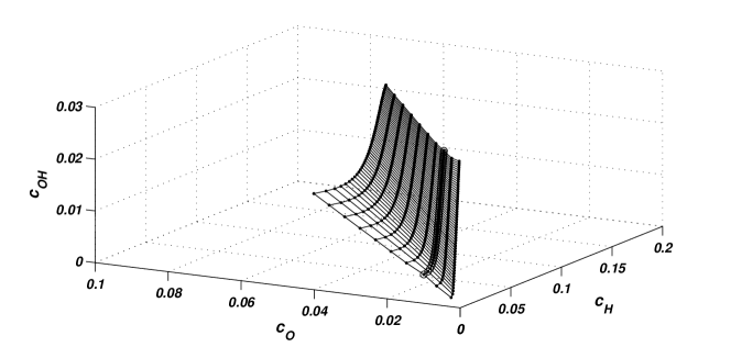
Refer to caption
Figure 9: The 2D SQEG constructed by using the straightforward extension with ε2=0.5103superscript𝜀20.5superscript103\varepsilon^{2}=0.5\cdot 10^{-3}: projection into the phase-subspace (cH,cO,cOHsubscript𝑐𝐻subscript𝑐𝑂subscript𝑐𝑂𝐻c_{H},c_{O},c_{OH}).

In order to get a 2D SQEG for that example, the straightforward extension was used as first strategy. Matrices 𝑫𝑫D and 𝑬𝑬E take now the form:

𝑫=[202101021011],𝑬=[0.5770.5680.2250.04820.06660.5360.006820.005950.02210.70.7130.423202101021011].formulae-sequence𝑫delimited-[]202101missing-subexpressionmissing-subexpressionmissing-subexpressionmissing-subexpressionmissing-subexpressionmissing-subexpressionmissing-subexpressionmissing-subexpressionmissing-subexpressionmissing-subexpressionmissing-subexpressionmissing-subexpressionmissing-subexpressionmissing-subexpression021011missing-subexpressionmissing-subexpressionmissing-subexpressionmissing-subexpressionmissing-subexpressionmissing-subexpressionmissing-subexpressionmissing-subexpressionmissing-subexpressionmissing-subexpressionmissing-subexpressionmissing-subexpressionmissing-subexpressionmissing-subexpression𝑬delimited-[]0.5770.5680.2250.04820.06660.536missing-subexpressionmissing-subexpressionmissing-subexpressionmissing-subexpressionmissing-subexpressionmissing-subexpressionmissing-subexpressionmissing-subexpressionmissing-subexpressionmissing-subexpressionmissing-subexpressionmissing-subexpressionmissing-subexpressionmissing-subexpression0.006820.005950.02210.70.7130.423missing-subexpressionmissing-subexpressionmissing-subexpressionmissing-subexpressionmissing-subexpressionmissing-subexpressionmissing-subexpressionmissing-subexpressionmissing-subexpressionmissing-subexpressionmissing-subexpressionmissing-subexpressionmissing-subexpressionmissing-subexpression202101missing-subexpressionmissing-subexpressionmissing-subexpressionmissing-subexpressionmissing-subexpressionmissing-subexpressionmissing-subexpressionmissing-subexpressionmissing-subexpressionmissing-subexpressionmissing-subexpressionmissing-subexpressionmissing-subexpressionmissing-subexpression021011missing-subexpressionmissing-subexpressionmissing-subexpressionmissing-subexpressionmissing-subexpressionmissing-subexpressionmissing-subexpressionmissing-subexpressionmissing-subexpressionmissing-subexpressionmissing-subexpressionmissing-subexpressionmissing-subexpressionmissing-subexpression\mbox{\boldmath$D$}=\left[{\begin{array}[]{*{20}c}2&0&2&1&0&1\\ 0&2&1&0&1&1\\ \end{array}}\right],{\kern 1.0pt}\mbox{\boldmath$E$}=\left[{\begin{array}[]{*{20}c}{-0.577}&{-0.568}&{0.225}&{0.0482}&{-0.0666}&{-0.536}\\ {0.00682}&{-0.00595}&{0.0221}&{-0.7}&{-0.713}&{0.423}\\ 2&0&2&1&0&1\\ 0&2&1&0&1&1\\ \end{array}}\right]. (65)

As suggested in the end of section 7.1, the procedure has been started from the equilibrium point and it was split in two subsequent steps. At the beginning, the system (57) was solved by imposing ε2=0.5103superscript𝜀20.5superscript103\varepsilon^{2}=0.5\cdot 10^{-3} and 𝒎~=𝒙ls2bold-~𝒎superscriptsubscript𝒙𝑙𝑠2\mbox{\boldmath$\tilde{m}$}=\mbox{\boldmath$x$}_{l}^{s2}: in this way, the grid nodes, denoted by circles, in Fig. 9 were obtained. In the second step, (57) was solved by starting from any circle: this time, the geometric constraints were ε2=0.5103superscript𝜀20.5superscript103\varepsilon^{2}=0.5\cdot 10^{-3} and 𝒎~=𝒙ls1bold-~𝒎superscriptsubscript𝒙𝑙𝑠1\mbox{\boldmath$\tilde{m}$}=\mbox{\boldmath$x$}_{l}^{s1}. During that step, in each circle, the horizontal dots of Fig. 9 were found, too.

8.2 The 2D flag extension

After that, also the flag extension procedure was applied. Now, the 1D spectral quasi equilibrium grid is needed. Matrices 𝑫𝑫D and 𝑬𝑬E are in this case:

𝑫=[202101021011],𝑬=[0.5770.5680.2250.04820.06660.536202101021011].formulae-sequence𝑫delimited-[]202101missing-subexpressionmissing-subexpressionmissing-subexpressionmissing-subexpressionmissing-subexpressionmissing-subexpressionmissing-subexpressionmissing-subexpressionmissing-subexpressionmissing-subexpressionmissing-subexpressionmissing-subexpressionmissing-subexpressionmissing-subexpression021011missing-subexpressionmissing-subexpressionmissing-subexpressionmissing-subexpressionmissing-subexpressionmissing-subexpressionmissing-subexpressionmissing-subexpressionmissing-subexpressionmissing-subexpressionmissing-subexpressionmissing-subexpressionmissing-subexpressionmissing-subexpression𝑬delimited-[]0.5770.5680.2250.04820.06660.536missing-subexpressionmissing-subexpressionmissing-subexpressionmissing-subexpressionmissing-subexpressionmissing-subexpressionmissing-subexpressionmissing-subexpressionmissing-subexpressionmissing-subexpressionmissing-subexpressionmissing-subexpressionmissing-subexpressionmissing-subexpression202101missing-subexpressionmissing-subexpressionmissing-subexpressionmissing-subexpressionmissing-subexpressionmissing-subexpressionmissing-subexpressionmissing-subexpressionmissing-subexpressionmissing-subexpressionmissing-subexpressionmissing-subexpressionmissing-subexpressionmissing-subexpression021011missing-subexpressionmissing-subexpressionmissing-subexpressionmissing-subexpressionmissing-subexpressionmissing-subexpressionmissing-subexpressionmissing-subexpressionmissing-subexpressionmissing-subexpressionmissing-subexpressionmissing-subexpressionmissing-subexpressionmissing-subexpression\mbox{\boldmath$D$}=\left[{\begin{array}[]{*{20}c}2&0&2&1&0&1\\ 0&2&1&0&1&1\\ \end{array}}\right],{\kern 1.0pt}\mbox{\boldmath$E$}=\left[{\begin{array}[]{*{20}c}{-0.577}&{-0.568}&{0.225}&{0.0482}&{0.0666}&{-0.536}\\ 2&0&2&1&0&1\\ 0&2&1&0&1&1\\ \end{array}}\right]. (66)

Starting from the equilibrium point 𝒄eqsuperscript𝒄𝑒𝑞\mbox{\boldmath$c$}^{eq}, the system (34) was solved by fixing ε2=3103superscript𝜀23superscript103\varepsilon^{2}=3\cdot 10^{-3} (see Fig. 10).

Refer to caption
Figure 10: 1D Spectral Quasi Equilibrium Grid with ε2=3103superscript𝜀23superscript103\varepsilon^{2}=3\cdot 10^{-3}: comparison with the 1D invariant grid obtained by MIG refinements.

The flag extension was used to get a 2D grid out of the 1D one. Now, the new matrix 𝑬𝑬E reads:

Refer to caption
Figure 11: The flag extension. (a) 2D SQEG (dots) extended from the 1D SQEG (circles). (b) 2D SQEG (dots) extended from the 1D invariant grid (circles). The grid spacing, in the second dimension, was ε2=1.5103superscript𝜀21.5superscript103\varepsilon^{2}=1.5\cdot 10^{-3}.
𝑬=[0.006820.005950.02210.70.7130.423202101021011],𝑬delimited-[]0.006820.005950.02210.70.7130.423missing-subexpressionmissing-subexpressionmissing-subexpressionmissing-subexpressionmissing-subexpressionmissing-subexpressionmissing-subexpressionmissing-subexpressionmissing-subexpressionmissing-subexpressionmissing-subexpressionmissing-subexpressionmissing-subexpressionmissing-subexpression202101missing-subexpressionmissing-subexpressionmissing-subexpressionmissing-subexpressionmissing-subexpressionmissing-subexpressionmissing-subexpressionmissing-subexpressionmissing-subexpressionmissing-subexpressionmissing-subexpressionmissing-subexpressionmissing-subexpressionmissing-subexpression021011missing-subexpressionmissing-subexpressionmissing-subexpressionmissing-subexpressionmissing-subexpressionmissing-subexpressionmissing-subexpressionmissing-subexpressionmissing-subexpressionmissing-subexpressionmissing-subexpressionmissing-subexpressionmissing-subexpressionmissing-subexpression\mbox{\boldmath$E$}=\left[{\begin{array}[]{*{20}c}{0.00682}&{-0.00595}&{0.0221}&{-0.7}&{-0.713}&{0.423}\\ 2&0&2&1&0&1\\ 0&2&1&0&1&1\\ \end{array}}\right],

while the Lyapunov function G𝐺G has the form:

G=i=16ci[ln(cici)1],𝐺superscriptsubscript𝑖16subscript𝑐𝑖delimited-[]subscript𝑐𝑖superscriptsubscript𝑐𝑖1G=\sum\nolimits_{i=1}^{6}{c_{i}\left[{\ln\left({\frac{{c_{i}}}{{c_{i}^{*}}}}\right)-1}\right]}, (67)

where 𝒄=[c1,,c6]superscript𝒄superscriptsubscript𝑐1superscriptsubscript𝑐6\mbox{\boldmath$c$}^{*}=[c_{1}^{*},...,c_{6}^{*}] is any 1D grid node which is extended in the second dimension (see Fig. 8). Figures 11(a)-(b) show two different 2D SQE-grids: the first one is obtained by extending the 1D SQE-grid, while in the second case the 1D invariant grid is used. In other words, the latter result was attained by the “hybrid procedure” QEGA𝑄𝐸𝐺𝐴QEGA + MIG𝑀𝐼𝐺MIG suggested in the end of section 7.2. For both cases, in the second dimension, the grid spacing was ε2=1.5103superscript𝜀21.5superscript103\varepsilon^{2}=1.5\cdot 10^{-3}.

8.3 The 2D GQEG and SEGQEG

Refer to caption
Figure 12: 1.case: k1+=2superscriptsubscript𝑘12k_{1}^{+}=2, k2+=1superscriptsubscript𝑘21k_{2}^{+}=1, k3+=1superscriptsubscript𝑘31k_{3}^{+}=1, k4+=103superscriptsubscript𝑘4superscript103k_{4}^{+}=10^{3}, k5+=103superscriptsubscript𝑘5superscript103k_{5}^{+}=10^{3}, k6+=102superscriptsubscript𝑘6superscript102k_{6}^{+}=10^{2}, ε2=0.45103superscript𝜀20.45superscript103\varepsilon^{2}=0.45\cdot 10^{3}. Two grids formed by 10×15101510\times 15 nodes. A 2D GQEG (dots) and a 2D invariant grid (circles) are reported. The grids are partially extended below the equilibrium point (square).

Finally, the GQEG and SEGQEG approximations are computed for the hydrogen oxidation reaction (60) (1.case). Here, the grid spacing is uniformly kept ε2=0.45103superscript𝜀20.45superscript103\varepsilon^{2}=0.45\cdot 10^{-3}. Each grid has 10×15101510\times 15 nodes and it is compared with both the SQEG (straightforward extension) of similar size (check Table 1) and the invariant one. The invariant grid was obtained by refining the approximations through the MIG procedure. All those grids lie quite close to each other. However, a “more pathological” case (2.case) is also analyzed (here the SQEG, far from the equilibrium, presents a remarkable deviation from the invariant grid): now the rate constant set is taken as k1+=20superscriptsubscript𝑘120k_{1}^{+}=20, k2+=1superscriptsubscript𝑘21k_{2}^{+}=1, k3+=1superscriptsubscript𝑘31k_{3}^{+}=1, k4+=103superscriptsubscript𝑘4superscript103k_{4}^{+}=10^{3}, k5+=103superscriptsubscript𝑘5superscript103k_{5}^{+}=10^{3}, k6+=102superscriptsubscript𝑘6superscript102k_{6}^{+}=10^{2}, while the equilibrium point coordinates still are given by (62).
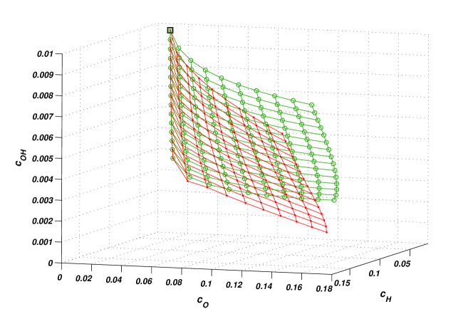
Refer to caption
Figure 13: 2.case: k1+=20superscriptsubscript𝑘120k_{1}^{+}=20, k2+=1superscriptsubscript𝑘21k_{2}^{+}=1, k3+=1superscriptsubscript𝑘31k_{3}^{+}=1, k4+=103superscriptsubscript𝑘4superscript103k_{4}^{+}=10^{3}, k5+=103superscriptsubscript𝑘5superscript103k_{5}^{+}=10^{3}, k6+=102superscriptsubscript𝑘6superscript102k_{6}^{+}=10^{2}, ε2=0.45103superscript𝜀20.45superscript103\varepsilon^{2}=0.45\cdot 10^{3}. Two grids formed by 10×15101510\times 15 nodes. A 2D GQEG (dots) and a 2D invariant grid (circles) are reported. The grids are partially extended below the equilibrium point (square).

For that case, the SQEG, GQEG and SEGQEG were constructed by choosing the grid spacing and size as for the previous case. Note that all the grids were partially extended only below the equilibrium point in the phase-space zone where they present the largest deviation from the invariant grid. This time those three approximations have a low invariance defect only near the equilibrium. In order to estimate how far each grid is from the invariant one, the following procedure is implemented. A 10×15101510\times 15 matrix, collecting in any grid node an invariance defect measure, is constructed. As suggested by [2], that local measure may be (𝚫,𝚫)/(𝑱,𝑱)𝚫𝚫𝑱𝑱\sqrt{\left({\mbox{\boldmath$\Delta$},\mbox{\boldmath$\Delta$}}\right)/\left({\mbox{\boldmath$J$},\mbox{\boldmath$J$}}\right)}, where 𝚫𝚫\Delta and 𝑱𝑱J are the invariance defect (11) and the vector field of (5), respectively. 𝚫𝚫\Delta is evaluated by using the thermodynamic projector (16). By averaging over all the invariance defect measures, the mean invariance defect is provided: results for both cases are condensed in Table 1. Note that the adopted invariance defect measure is dimensionless as it compares the invariance defect with the vector field. Calculations prove that the GQEG is better than the SQEG (straightforwardly extended); nevertheless the SEGQEG construction, since it requires a much lower computational effort and still has an error similar to the GQEG, is recommended when the SQEG is considered not satisfactory (e.g. big mean defect).

1.case 2.case
SQEG 0.318 0.645
GQEG 0.238 0.460
SEGQEG 0.303 0.491
Table 1: Mean invariance defect (dimensionless): three approximations of the invariant grid under comparison for the hydrogen oxidation reaction. In 1.case, the parameter set is: k1+=2superscriptsubscript𝑘12k_{1}^{+}=2, k2+=1superscriptsubscript𝑘21k_{2}^{+}=1, k3+=1superscriptsubscript𝑘31k_{3}^{+}=1, k4+=103superscriptsubscript𝑘4superscript103k_{4}^{+}=10^{3}, k5+=103superscriptsubscript𝑘5superscript103k_{5}^{+}=10^{3}, k6+=102superscriptsubscript𝑘6superscript102k_{6}^{+}=10^{2}, ε2=0.45103superscript𝜀20.45superscript103\varepsilon^{2}=0.45\cdot 10^{3}. In 2.case, the parameter set is: k1+=20superscriptsubscript𝑘120k_{1}^{+}=20, k2+=1superscriptsubscript𝑘21k_{2}^{+}=1, k3+=1superscriptsubscript𝑘31k_{3}^{+}=1, k4+=103superscriptsubscript𝑘4superscript103k_{4}^{+}=10^{3}, k5+=103superscriptsubscript𝑘5superscript103k_{5}^{+}=10^{3}, k6+=102superscriptsubscript𝑘6superscript102k_{6}^{+}=10^{2}, ε2=0.45103superscript𝜀20.45superscript103\varepsilon^{2}=0.45\cdot 10^{3}.

9 Conclusions

In this paper, the problem of Quasi Equilibrium Manifold approximation by means of a grid description is addressed. To this end, the notion of Quasi Equilibrium Grid (QEG) is introduced and a proper algorithm to construct it, in any dimension, is suggested (QEGA). It has been shown, through illustrative examples, that the QEGA gives a very good QEM approximation without facing the analytical difficulties of Lagrange multipliers method implementation in large dimension. Since the QEGA is a completely numerical procedure, it reveals particularly suitable for providing the MIG procedure with the first SIM approximation. As it has been illustrated, some proper hybrid procedures QEGA𝑄𝐸𝐺𝐴QEGA + MIG𝑀𝐼𝐺MIG, where both methods are alternatively used, allow to obtain accurate SIM approximations. It was proved that two special QEGA𝑄𝐸𝐺𝐴QEGA + MIG𝑀𝐼𝐺MIG procedures deliver enhanced approximations of SIM: the Guided Quasi Equilibrium Grid and the Symmetric Entropic Guided Quasi Equilibrium Grid. Here, we want to stress the two major advantages of the method proposed. First of all, it is a completely numerical algorithm which only deals with nodes sets. Moreover, it is a local construction: namely, the computation of a new node 𝒄n+1subscript𝒄𝑛1\mbox{\boldmath$c$}_{n+1}, which has to be added to the grid, only depends on the previous neighbor 𝒄nsubscript𝒄𝑛\mbox{\boldmath$c$}_{n}. Those two points make the QEG construction suitable for numerical applications and parallel realizations. Finally, it is not excluded that the QEGA is applicable not only for model reduction, but in some very different fields, too. Indeed, it was mentioned that the QEM notion already is exploited for some applications in Lattice Boltzmann schemes simulations. More generally, the QEGA is a numerical tool which can be used to find a grid-based approximation for the locus of minima of a convex function under some linear constraints. In this paper we focused only on the geometry of the model reduction, that is, construction of slow invariant manifolds approximations. The implementation of grid-based integrators for dynamic equations will be presented in a separate publication.

10 Acknowledgments

Prof. A. N. Gorban is gratefully acknowledged for the fruitful discussions about the concept of Quasi Equilibrium Manifold and for suggesting the reaction mechanism (39). We thank Prof. K. B. Bouluochos, Dr. C. E. Frouzakis for several discussions and suggestions. This work was partially supported by SNF, Project 200021-107885/1 (E.C.) and by BFE, Project 100862 (I.V.K.).

References

  • [1] A. N. Gorban, I. V. Karlin, Method of invariant manifold for chemical kinetics, Chem. Eng. Sci. 58 4751-4768 (2003).
  • [2] E. Chiavazzo, A. N. Gorban, I. V. Karlin, Comparison of invariant manifolds for model reduction in chemical kinetics, Comm. in Comput. Physics Vol. 2, No. 5, pp. 964-992 (2007).
  • [3] A. N. Gorban, I. V. Karlin, A. Y. Zinovyev, Invariant grids for reaction kinetics, Physica A 333 106-154 (2004).
  • [4] A. N. Gorban, I. V. Karlin, Invariant Manifolds for Physical and Chemical Kinetics, Lect. Notes Phys. 660 (Springer Berlin Heidelberg 2005), doi: 10.1007/b98103.
  • [5] A. N. Gorban, I. V. Karlin, V. B. Zmievskii, T.F.Nonnenmacher, Relaxational trajectories: global approximations, Physica A 231 648-672 (1996).
  • [6] I. V. Karlin, A. Ferrante, H. C. Öttinger, Perfect entropy functions of the lattice Boltzmann method, Europhys. Lett. 47, 182-188 (1999).
  • [7] S. Arcidiacono, J. Mantzaras, S. Ansumali, I. V. Karlin, C. Frouzakis, K. B. Boulouchos, Phys. Rev. E 74, 056707 (2006).
  • [8] A. N. Gorban, I.V.Karlin, Thermodynamic parametrization. Physica A 190 393-404 (1992).
  • [9] U. Maas, S. B. Pope, Simplifying Chemical Kinetics: Intrinsic Low-Dimensional Manifolds in Composition Space, Comb. and Flame 88 239-264 (1992).
  • [10] V. Bykov, I. Goldfarb, V. Gol’dshtein, U. Maas, On a modified version of ILDM approach: asymptotic analysis based on integral manifolds, IMA Jour. of Applied Math. 1-24 (2005).
  • [11] S. H. Lam, D. A. Goussis, Conventional asymptotic and computational singular perturbation for symplified kinetics modelling , in: M.O. Smooke (Ed.), Reduced Kinetic Mechanisms and Asymptotic Approximations for Methane-Air Flames, Springer Lecture Notes, (Springer Berlin 1991), pp. 227-242.
  • [12] S. H. Lam, D. A. Goussis, The CSP Method for Simplifying Kinetics, Intern. Jour. of Chemical Kinetics 26 461-486 (1994).
  • [13] D. A. Goussis, M. Valorani, An efficient iterative algorithm for the approximation of the fast and slow dynamics of stiff systems, Jour. of Computational Physics 214 316-346 (2006).
  • [14] I. G. Kevrekidis, C. W. Gear, J. M. Hyman, P. G. Kevrekidis, O. Runborg, C. Theodoropoulos, Equation-free: Coarse-grained Multiscale Computation Enabling Microscopic Simulators to Perform System-level Analysis, Comm. Math. Sci. 1 715-762 (2003).
  • [15] A. M. Lyapunov, The general problem of the stability of motion, Taylor & Francis, London, (1992).
  • [16] N. Kazantzis, Singular PDEs and the problem of finding invariant manifolds for nonlinear dynamical systems. Phys. Lett. A 272, 257-263 (2000).
  • [17] J. C. Robinson, A concise proof of the “geometric” construction of inertial manifolds, Phy. Lett. A 200, 415-417 (1995).
  • [18] L. B. Ryashko, E. E. Shnol, On exponentially attracting invariant manifolds of ODEs, Nonlinearity 16, 147-160 (2003).
  • [19] R. S. MacKay, Slow Manifolds, in: Energy Localisation and Transfer, ed. by T. Dauxois, A. Litvak-Hinenzon, R. S. MacKay, A. Spanoudaki (World Sci., 2004), 149-192.
  • [20] A. N. Gorban, I. V. Karlin, Uniqueness of thermodynamic projector and kinetic basis of molecular individualism, Physica A 336, 3-4, 391–432 (2004).
  • [21] P. D. Christofides, P. Daoutidis, Finite-dimensional control of parabolic PDE systems using approximate inertial manifolds, J. Math. An. & Appl. 216, 398-420 (1997).
  • [22] A. Degenhard, J. Rodriguez-Laguna, Projection Operators for Nonlinear Evolutionary Dynamics, SIAM Multiscale Modeling and Simulation 4, 641-663 (2005).
  • [23] H. G. Kaper, T. J. Kaper, Asymptotic analysis of two reduction methods for systems of chemical reactions, Physica D 165 66-93 (2002).
  • [24] N. Kazantzis, Singular PDEs and the problem of finding invariant manifolds for nonlinear dynamical systems, Physics Letters, A272(4), 257-263 (2000).
  • [25] M. R. Roussel, S. J. Fraser, On the geometry of transient relaxation, J. Chem. Phys. 94, 7106-711 (1991).
  • [26] M. R. Roussel, S. J. Fraser, Geometry of the steady-state approximation: Perturbation and accelerated convergence methods, J. Chem. Phys. 93, 1072-1081 (1990).
  • [27] S. J. Fraser, The steady state and equilibrium approximations: A geometrical picture, J. Chem. Phys. 88 4732-4738 (1988).