One-dimensional Rydberg Gas in a Magnetoelectric Trap

Abstract

We study the quantum properties of Rydberg atoms in a magnetic Ioffe-Pritchard trap which is superimposed by a homogeneous electric field. Trapped Rydberg atoms can be created in long-lived electronic states exhibiting a permanent electric dipole moment of several hundred Debye. The resulting dipole-dipole interaction in conjunction with the radial confinement is demonstrated to give rise to an effectively one-dimensional ultracold Rydberg gas with a macroscopic interparticle distance. We derive analytical expressions for the electric dipole moment and the required linear density of Rydberg atoms.

Because of their widely tunable properties, ultracold atomic gases provide the ideal playground to model and study complex many body systems. The interatomic interaction can be tailored using Feshbach-resonances and magnetic, optical, and electric fields can be applied in order to generate virtually any external potential. Famous examples for the versatility are the demonstration of the Mott-Insulator to superfluid phase-transition of ultracold atoms in an optical lattice Bloch02 , the BEC-BCS crossover in a gas of ${}^{\text{6}}$Li Chin04 , or the Kosterlitz-Thouless phase transition studied within a two-dimensional Bose-Einstein condensate Hadzibabic06 . Traditionally, there is a great interest in studying systems with reduced spatial dimensions, such as the latter example. One paradigm is constituted by the work of Lieb and Liniger who were the first to solve the system of pointlike interacting bosons in one dimension using Bethe’s ansatz Lieb63 . In the limit of an infinitely strong interparticle interaction strength, a so-called Tonks-Girardeau gas emerges GirardeauParedes .

Besides gases of ground state atoms, particularly Rydberg gases represent excellent systems to study the influence of a strong interparticle interaction on the dynamics of many-particle systems. Due to the large displacement of the ionic core and the valence electron, Rydberg atoms can develop a large electric dipole moment leading to a strong and long-ranged dipole-dipole interaction among them Gallagher . However, unlike ground state atoms Rydberg atoms suffer from radiative decay and hence the mutual interaction time is limited by the lifetime of the electronically excited state. But still, in so-called frozen Rydberg gases, where the timescale of the atomic motion is much longer than the radiative lifetime, exciting effects like the dipole-blockade LukinTong or resonant population transfer PilletGallagher have been observed.

Several works have focused on the important issue of trapping Rydberg atoms based on electric Hyafil04 , optical Dutta00 , or strong magnetic fields Choi05_1 . Due to the high level density and the strong spectral fluctuations with spatially varying fields, trapping or manipulation in general is a delicate task. This holds particularly for the case where both the center of mass and internal motion are of quantum nature. Moreover, the inhomogeneous external fields lead to an inherent coupling of these motions. Addressing this regime, it has been recently theoretically shown that Rydberg atoms can be tightly confined and prepared in long-lived electronic states in a magnetic Ioffe-Pritchard (IP) trap Hezel which can be miniaturized using so-called atomchips FolmanFortagh . Here we use the IP configuration as a key ingredient in order to ’prepare’ and study a one-dimensional (1D) Rydberg gas. Specifically, we propose a modified IP trap, a magneto-electric trap, which offers confining potential energy surfaces for the atomic center of mass (c.m.) motion in which the atoms possess an oriented permanent electric dipole moment. We derive analytical expressions for the dipole-dipole interaction among trapped Rydberg atoms and estimate below which Rydberg atom density a 1D Rydberg gas is expected to form. Moreover, we estimate the lifetime of such a gas.

Proceeding along the lines of Refs. Hezel ; Lesanovsky05_03 , we employ a two-body approach in order to model an alkali metal atom in a Rydberg state. We assume the single valence electron and the ionic core (mass $M_{c}$) to interact via a pure Coulomb potential. While the inclusion of the fine-structure and quantum defects can be readily done, it turns out not to be necessary for high angular momentum electronic states in the regime we are focussing on Hezel . The IP field configuration is given by $\mathbf{B}(\mathbf{x})=B\mathbf{e}_{3}+\mathbf{B}_{\text{lin}}(\mathbf{x})$ with $\mathbf{B}_{\text{lin}}(\mathbf{x})=G\left[x_{1}\mathbf{e}_{1}-x_{2}\mathbf{e}_{2}\right]$ and the vector potential reads $\mathbf{A}(\mathbf{x})=\mathbf{A}_{\mathrm{c}}(\mathbf{x})+\mathbf{A}_{\mathrm{lin}}(\mathbf{x})$ with $\mathbf{A}_{\mathrm{c}}(\mathbf{x})=\frac{B}{2}\left[x_{1}\mathbf{e}_{2}-x_{2}\mathbf{e}_{1}\right]$ and $\mathbf{A}_{\mathrm{lin}}(\mathbf{x})=Gx_{1}x_{2}\mathbf{e}_{3}$, where $B$ and $G$ are the Ioffe field strength and the gradient, respectively. In addition, we apply a homogeneous electric field pointing in the $x_{1}$-direction of the laboratory frame $\mathbf{F}=F\mathbf{e}_{1}$. After introducing relative and c.m. coordinates ($\mathbf{r}$ and $\mathbf{R}$) and employing the unitary transformation $U=\exp\left[i\frac{B}{2}\mathbf{e}_{3}\times\mathbf{r}\cdot\mathbf{R}\right]$, the Hamiltonian describing the Rydberg atom becomes (atomic units are used unless stated otherwise)

$$H_{\text{IPE}} = H_{A}+\mathbf{A}_{\text{c}}(\mathbf{r})\cdot\mathbf{p}+\frac{\mathbf{\mathbf{P}}^{2}}{2M_{c}}-\mbox{\boldmath$\mu$}_{N}\cdot\mathbf{B}(\mathbf{R})+\mathbf{F}\cdot\mathbf{r}$$ (1)

$$-\mbox{\boldmath$\mu$}_{e}\cdot\mathbf{B}(\mathbf{R}+\mathbf{r})+\mathbf{A}_{\text{lin}}(\mathbf{R}+\mathbf{r})\cdot\mathbf{p}.$$

Here, $H_{A}=\frac{\mathbf{p}^{2}}{2}-\frac{1}{r}$ is the Hamiltonian of a hydrogen atom possessing the energies $E_{n}=-\frac{1}{2}n^{-2}$. The second term denotes the energy of the electron in the homogeneous Ioffe field due to its orbital motion. The following two terms of $H_{\text{IPE}}$ describe the motion of a point-like particle possessing the magnetic moment $\mbox{\boldmath$\mu$}_{N}$ in the presence of the field $\mathbf{B}$. The magnetic moments are connected to the electronic spin $\mathbf{S}$ and the nuclear spin $\mathbf{\Sigma}$ according to $\mbox{\boldmath$\mu$}_{e}=-\mathbf{S}$ and $\mbox{\boldmath$\mu$}_{N}=-\frac{g_{N}}{2M_{c}}\mathbf{\Sigma}$, with $g_{N}$ being the nuclear $g$-factor. We neglect the term involving $\mbox{\boldmath$\mu$}_{N}$ in the following due to the large nuclear mass. The electric field interaction, which in case of a neutral two-body system couples only to the relative coordinates, gives rise to the fifth term. The last two terms of $H_{\text{IPE}}$ are spin-field and motionally induced terms coupling the electronic and c.m. dynamics. We focus on a parameter regime which allows us to neglect the diamagnetic interactions Hezel .

In order to find the stationary states of the Hamiltonian (1), we assume that neither the magnetic nor the electric field causes couplings between electronic states with different principal quantum number $n$. In this case we can consider each $n$-manifold separately and may represent the Hamiltonian (1) in the space of the $2n^{2}$ states which span the $n$-manifold under investigation. The parameter range in which this approximation is valid has been thoroughly discussed in Refs. Hezel ; Schmidt07 . Because of the translational symmetry of the IP and the electric field, the axial c.m. motion along $Z$ can be separated from the transversal motion in the $X$-$Y$ plane. If we omit the energy offset $E_{n}$ and introduce scaled c.m. coordinates ($\mathbf{R}\rightarrow\gamma^{-\frac{1}{3}}\mathbf{R}$ with $\gamma=GM_{c}$) while scaling the energy unit with $\epsilon_{\mathrm{scale}}=\gamma^{\frac{2}{3}}/M_{c}$, we arrive at the Hamiltonian

$$\mathcal{H}=\frac{P_{1}^{2}+P_{2}^{2}}{2}+\mbox{\boldmath$\mu$}\cdot\mathbf{G}+\gamma^{-\frac{2}{3}}M_{c}\left[\mathcal{H}_{m}+\mathcal{H}_{e}\right].$$ (2)

This Hamiltonian governs the transversal c.m. as well as the electronic dynamics and involves the effective magnetic field $\mathbf{G}=X\mathbf{e}_{1}-Y\mathbf{e}_{2}+\gamma^{-\frac{2}{3}}M_{c}B\mathbf{e}_{3}$. The symbols $\mu$, $\mathcal{H}_{m}$, and $\mathcal{H}_{e}$ are the $2n^{2}$-dimensional matrix representations of the operators $\frac{1}{2}\left[\mathbf{L}+2\mathbf{S}\right]$, $H_{m}=\mathbf{A}_{\mathrm{lin}}(\mathbf{r})\cdot\mathbf{p}+\mathbf{B}_{\mathrm{lin}}(\mathbf{r})\cdot\mathbf{S}$, and the electric field interaction $H_{e}=Fx$, respectively (we introduced $\mathbf{L}=\mathbf{r}\times\mathbf{p}$). A thorough interpretation of this Hamiltonian in the absence of $\mathcal{H}_{e}$ is provided in Ref. Hezel . In order to solve the corresponding Schrödinger equation we employ an adiabatic approach. To this end an unitary transformation $U(X,Y)$ which diagonalizes the last two (matrix) terms of the Hamiltonian is applied, $U^{\dagger}(X,Y)(\mbox{\boldmath$\mu$}\cdot\mathbf{G}+\gamma^{-\frac{2}{3}}M_{c}\left[\mathcal{H}_{m}+\mathcal{H}_{e}\right])U(X,Y)=E_{\alpha}(X,Y)$. Since $U(X,Y)$ depends on the c.m. coordinates, the transformed kinetic energy term involves non-adiabatic (off-diagonal) coupling terms which can be neglected in our parameter regime Hezel . We are thereby led to a set of $2n^{2}$ decoupled differential equations governing the adiabatic c.m. motion within the individual two-dimensional energy surfaces $E_{\alpha}(X,Y)$, i.e., the surfaces $E_{\alpha}(X,Y)$ serve as potentials for the c.m. motion of the atom.

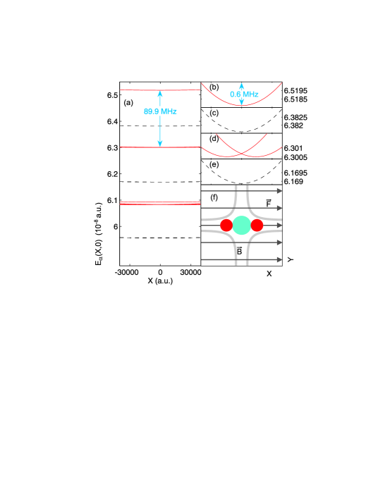
Figure 1: (Color online) Potential energy surfaces of the c.m. motion of a ⁸⁷Rb atom ($n=30$) in an IP trap with $B=10\,\text{G}$, $G=10\,\text{Tm}^{-1}$. Dashed lines: $F=0$, solid lines: $F=5.14\,\text{Vm}^{-1}$. An overview of the seven energetically highest potential curves is shown in panel (a). Magnified views of the uppermost (b,c) and next lower ones (d,e) are also provided. The range of the $X$-coordinate, corresponding to $2.1\mu\text{m}$, is the same for each subfigure (a)-(e). The total field configuration is sketched in panel (f) where the circles depict the locations of the minima of the uppermost (big circle) and the two adjacent lower-lying (small circles) c.m. surfaces. The magnetic field lines are indicated in gray while the electric field is sketched by black arrows.

In Fig. 1 we present intersections along the $X$-direction of such potential surfaces for $B=10\,\text{G}$, $G=10\,\text{Tm}^{-1}$ and $n=30$ in the case of ⁸⁷Rb. For zero electric field strength (dashed lines), the potential curves are organized in groups which are energetically well-separated by a gap of $\gamma^{-\frac{2}{3}}M_{c}B=89.9$ MHz. The uppermost surface is non-degenerate and provides an approximately harmonic confinement with a trap frequency of $\omega=G\sqrt{n/2BM_{c}}=13.9\,$kHz corresponding to $0.1\,\mu\text{K}$. The two adjacent lower surfaces are degenerate and also approximately harmonic. As soon as an electric field is applied, all surfaces are shifted considerably in energy. This is visible from the solid curves in Fig. 1 for which an electric field of strength $F=5.14\,\text{Vm}^{-1}$ is applied. The shapes of the potentials are barely affected by the electric field such that Rydberg states which were trapped in a pure IP configuration remain confined also in the magneto-electric trap. Moreover, adding the electric field leads to non-trivial effects: The second and third surface, which were almost degenerate in the absence of the electric field, are now shifted in opposite ways along the $x_{1}$-direction. All surfaces shown provide a harmonic confinement with a trap frequency $\omega$ also in the $x_{2}$-direction. We remark that the chosen parameter set does not generate an extreme constellation hence an even stronger confinement can be achieved without invalidating the applied approximations Hezel .

Let us now investigate the electronic properties of a Rydberg atom being trapped in the uppermost potential surface. For $F=0$ and sufficiently large values of $B$, this surface is formed almost exclusively by the highest possible electronic angular momentum state, i.e., $l=n-1$ Hezel . If $F$ is increased, electronic states with smaller $l$ will be inevitably admixed to the electronic state belonging to this energy surface. An interesting property to investigate is hence the electric dipole moment of trapped Rydberg atoms: While for $F=0$ the electronic states are almost pure parity eigenstates and therefore exhibit almost no electric dipole, the admixture of lower $l$ states to the uppermost surface in the presence of the field is expected to give rise to a non-vanishing expectation value of the dipole operator. Indeed, this becomes evident in Fig. 2 where the uppermost potential surface and the three components of the expectation value of the electric dipole operator $\mathbf{D}(\mathbf{R})=\left<\mathbf{r}\right>(\mathbf{R})$ are shown (same parameters as in Fig. 1). It can be clearly seen that a permanent dipole moment is established whose dominant contribution points along the electric field vector.

In order to study the dependence of $\mathbf{D}(\mathbf{R})$ on the field strengths $F$ and $B$ as well as on the degree of electronic excitation, we use perturbation theory. In the limit of a large Ioffe field strength $B$ the unitary transformation which diagonalizes the Hamiltonian (2) can be written explicitly as $U_{\mathbf{r}}=e^{-i\alpha(L_{x}+S_{x})}e^{-i\beta(L_{y}+S_{y})}$ with $\sin\alpha=-Y\,|\mathbf{G}|^{-1}$, $\cos\alpha=\sqrt{|\mathbf{G}|^{2}-Y^{2}}\,|\mathbf{G}|^{-1}$, $\sin\beta=X\,(|\mathbf{G}|^{2}-Y^{2})^{-\frac{1}{2}}$ and $\cos\beta=\gamma^{-\frac{2}{3}}M_{c}B\,(|\mathbf{G}|^{2}-Y^{2})^{-\frac{1}{2}}$. This transformation rotates the $z$-axis into the local magnetic field direction where $\alpha$ and $\beta$ denote the rotation angles. Using this result we find up to first order in $F/B$ the electric dipole moment (in atomic units)

$$\mathbf{D}(\mathbf{R})=\frac{9}{2}\frac{F}{B}n^{2}(n-1)\left(\begin{array}[]{c}\cos\beta\\ \sin\beta\sin\alpha\\ \sin\beta\cos\alpha\\ \end{array}\right).$$ (6)

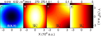
Figure 2: (Color online) (a) Uppermost electronic potential surface for the c.m. motion of ⁸⁷Rb in the $n=30$ multiplet and the parameters used in Fig. 1. (b-d) Components of the electronic dipole moment $\mathbf{D}(\mathbf{R})$ in atomic units. One recognizes the clear alignment of the electric dipole moment along the electric field vector. The numerically calculated values of $\mathbf{D}(\mathbf{R})$ are to good accuracy reproduced by Eq. (6).

We note that $\mathbf{D}(\mathbf{R})$ scales proportional to the third power of the principal quantum number and can therefore gain a significant magnitude even if the ratio $F/B$ is small. Good agreement of Eq. (6) with the calculated data presented in Fig. 2 is found; e.g., in the vicinity of the minimum of the potential surface ($X=Y=0$) we find an exact value of $D_{x}=270$ whereas the expression (6) yields $276$. For the remaining components Eq. (6) yields zero at the origin. For smaller ratios of $F/B$, even better agreement can be achieved.

Because of the dependence on the angles $\alpha$ and $\beta$, the dipole moment depends weakly on the quantum state of the c.m. motion. However, since the field configuration is translationally symmetric the electric dipole moment is independent of the $Z$-position of the Rydberg atoms in the trap. If we now consider two transversally confined atoms in the same trap at the longitudinal positions $Z_{A}$ and $Z_{B}$, we can write for their dipole-dipole interaction

$$V_{\mathrm{D}}(\mathbf{R}_{A},\mathbf{R}_{B})=\frac{1}{|\mathbf{R}_{A}-\mathbf{R}_{B}|^{3}}\Big{(}\mathbf{D}(\mathbf{R}_{A})\cdot\mathbf{D}(\mathbf{R}_{B})$$

$$-3\left[\mathbf{D}(\mathbf{R}_{A})\cdot\mathbf{e}\right]\left[\mathbf{D}(\mathbf{R}_{B})\cdot\mathbf{e}\right]\Big{)}\approx\frac{\mathbf{D}(\mathbf{R}_{A})\cdot\mathbf{D}(\mathbf{R}_{B})}{|Z_{A}-Z_{B}|^{3}}$$ (7)

where $\mathbf{e}$ denotes the interparticle unit vector. The approximation in Eq. (7) holds due to the orientation of the dipoles and the assumption that $|Z_{A}-Z_{B}|$ is large compared to the transversal oscillator length of the trap. These conditions moreover ensure a minimal coupling of the transversal and longitudinal motion. Using this approximation one can estimate the interaction energy of one atom being part of an infinite atomic chain with an interparticle spacing $a$. One finds

$$E_{\mathrm{int}}=2\frac{\mathbf{D}^{2}(0)}{a^{3}}\sum_{k=1}^{\infty}k^{-3}=\frac{81}{2a^{3}}\frac{F^{2}}{B^{2}}n^{4}(n-1)^{2}\zeta(3)$$ (8)

with the Riemann zeta function $\zeta(x)$. Here we have approximated $\mathbf{D}^{2}(\mathbf{R})\approx\mathbf{D}^{2}(0)$ since the dipole moment barely varies in the vicinity of $X=Y=0$. If the interaction energy $E_{\mathrm{int}}$ is smaller than the transversal trap frequency $\omega$, we can assume that the interacting atoms remain in the transversal ground state: This is considered the 1D regime. The linear density below which a 1D Rydberg gas is expected to form is then given by

$$N_{\mathrm{1D}}=\frac{\sqrt{B}}{3}\left[3\sqrt{\frac{M_{c}}{2}}\frac{F^{2}}{G}\,\zeta(3)\,n^{7/2}(n-1)^{2}\right]^{-\frac{1}{3}}\;.$$ (9)

Above this density, excited transversal c.m. states might be populated resulting in a quasi 1D Rydberg gas which is certainly of interest on its own. For our parameter set, we obtain a minimal interparticle spacing $a=43\,\mu$m; hence a chain of 1 mm in length contains 23 particles. This density can be further increased by either increasing the magnetic field gradient and/or decreasing the electric field strength: At $B=10\,$G, $G=100\,\text{Tm}^{-1}$, and $F=0.514\,\text{Vm}^{-1}$ a chain of the same length would contain 230 Rydberg atoms.

Finally, the issue of radiative decay has to be addressed. Since the electric field admixes merely a few $l=m$ states ($l<n-1$) to the electronic wave function of the uppermost surface, its circular character remains dominant resulting in one prevalent decay channel. For an atom being confined to the energy surface which is shown in Fig. 2, we have calculated a lifetime of $\tau\approx 2.1\,$ms which is in good agreement with the corresponding field-free result $\tau(n,n-1)\approx\frac{3}{2c^{2}}\left(\frac{n}{\alpha}\right)^{5}$ Jentschura05 . Corrections to this bare decay rate are found to be of the order of $(F/B)^{2}n^{3}$. Due to the scaling proportional to $n^{5}$, the lifetime can be significantly enhanced by exciting to a higher principal quantum number $n$. In addition, it can be further prolonged by establishing an adapted experimental setup which inhibits the electromagnetic field mode at the dominant transition frequency Hulet85 . At the same time, a cryogenic environment will diminish the undesirable effect of stimulated (de-)excitation by blackbody radiation. The timescale of the dynamics of the Rydberg chain on the other hand depends on the field strengths via the dipole moment and the interparticle spacing: A harmonic approximation of the dipole-dipole interaction yields the one-particle oscillator frequency $\omega_{\text{dd}}=\sqrt{24\,\mathbf{D}^{2}(0)/M_{c}a^{5}}$. As an example, the field configuration $B=10\,$G, $G=100\,\text{Tm}^{-1}$, and $F=0.514\,\text{Vm}^{-1}$ yields a timescale of less than 1 ms.

Let us now briefly comment on the realization of such a Rydberg gas which is certainly a challenging experimental task. One could start from an extremely dilute ultracold atomic gas prepared in an elongated IP trap. For transferring ground state atoms to high angular momentum Rydberg states, techniques such as crossed electric and magnetic fields or rotating microwave fields can be employed, see Ref. Lutwak97 and references therein. For low angular momentum states, trapping and the formation of a permanent dipole represent still an open question since quantum defects, spin-orbit coupling and reduced radiative lifetimes have to be taken into account. During the preparation, the excitation lasers have to be focussed such that Rydberg atoms emerge only at positions separated by the interparticle spacing $a$ which is required to meet the criterion (9). Since $a$ is in the order of several $\mu$m, which can be resolved optically, this should be feasible. The large value of $a$ moreover ensures that the mutual ionization due to the overlap of the electronic clouds of two atoms does not occur. For our circular states with $n=30$, the atomic extension can be estimated by $\langle r\rangle\approx n^{2}=48$ nm and is thus orders of magnitude smaller than the corresponding value of $a$ for our field configuration. In order to probe the dynamics of the resultant Rydberg chain, one can field-ionize the atoms: From the spatially resolved electron signal a direct mapping to the positions of the Rydberg atoms should be possible.

In conclusion, we demonstrated that in a magneto-electric trap Rydberg states can be confined in electronic states exhibiting a permanent electric dipole moment of hundreds of Debyes. Analytical expressions for the density which is required to enter the 1D regime were calculated. Moreover, we pointed out that the lifetime of the Rydberg states is sufficiently long to probe the dynamics of the interacting gas. This regime is complementary to the well-studied frozen Rydberg gases where mechanical atom-atom interaction effects can hardly be probed. The potential of the proposed magneto-electric trap is by far not entirely exhausted; e.g., one could think of using the double-well structure which is visible in Fig. 1(d) in order to realize two coupled dipolar Rydberg chains.

This work was supported by the German Research Foundation (DFG) under the contract SCHM 885/10-2 and within the framework of the Excellence Initiative through the Heidelberg Graduate School of Fundamental Physics (GSC 129/1). M.M. acknowledges support from the Landesgraduiertenförderung Baden-Württemberg.

References

- (1) M. Greiner et al., Nature 415, 39 (2002)
- (2) C. Chin et al., Science 305, 1128 (2004)
- (3) Z. Hadzibabic et al., Nature 441, 1118 (2006)
- (4) E. H. Lieb and W. Liniger, Phys. Rev. 130, 1605 (1963); E. H. Lieb, ibid. 130, 1616 (1963)
- (5) M. Girardeau, J. Math. Phys. 1, 516 (1960); B. Paredes et al., Nature 429, 277 (2004)
- (6) T.F. Gallagher, Rydberg Atoms, Cambridge University Press 1994
- (7) M. D. Lukin et al., Phys. Rev. Lett. 87, 037901 (2001); D. Tong et al., ibid. 93, 063001 (2004)
- (8) W. R. Anderson, J. R. Veale, and T. F. Gallagher Phys. Rev. Lett. 80, 249 (1998); I. Mourachko et al., ibid. 80, 253 (1998)
- (9) P. Hyafil et al., Phys. Rev. Lett. 93, 103001 (2004)
- (10) S.K. Dutta et al., Phys. Rev. Lett. 85, 5551 (2000)
- (11) J.-H. Choi et al., Phys. Rev. Lett. 95, 243001 (2005)
- (12) B. Hezel, I. Lesanovsky, and P. Schmelcher, Phys. Rev. Lett. 97, 223001 (2006); arXiv:0705.1299v2
- (13) J. Fortagh and C. Zimmermann, Rev. Mod. Phys. 79, 235 (2007); R. Folman et al., Adv. At. Mol. Opt. Phys. 48, 263 (2002)
- (14) I. Lesanovsky and P. Schmelcher, Phys. Rev. Lett. 95, 053001 (2005)
- (15) U. Schmidt, I. Lesanovsky, and P. Schmelcher, J. Phys. B 40, 1003 (2007)
- (16) U. D. Jentschura et al., J. Phys. B 38, S97 (2005)
- (17) R. G. Hulet, E. S. Hilfer, and D. Kleppner, Phys. Rev. Lett. 55, 2137 (1985)
- (18) R. Lutwak et al., Phys. Rev. A 56, 1443 (1997)