X-ray source counts in the XMM-COSMOS survey

Abstract

We present the analysis of the source counts in the XMM-COSMOS survey using data of the first year of XMM-Newton observations. The survey covers $\sim$2 deg² within the region of sky bounded by $9^{h}57.5^{m}<R.A.<10^{h}03.5^{m}$; $1^{d}27.5^{m}<DEC<2^{d}57.5^{m}$ with a total net integration time of 504 ks. Using a maximum likelihood algorithm we detected a total of 1390 sources at least in one band. Using Monte Carlo simulations to estimate the sky coverage we produced the logN-logS relations. These relations have been then derived in the 0.5–2 keV, 2–10 keV and 5–10 keV energy bands, down to flux limits of 7.2$\times$10^-16 erg cm^-2 s^-1, 4.0$\times$10^-15 erg cm^-2 s^-1 and 9.7$\times$10^-15 erg cm^-2 s^-1, respec tively. These relations have been compared to previous X-ray survey and to the most recent X-ray background model finding an excellent agreement. The slightly different normalizations observed in t he source counts of COSMOS and previous surveys can be largely explained as a co mbination of low counting statistics and cosmic variance introduced by the large scale structure.

1. Introduction

A solid knowledge of the X-ray source counts is fundamental to fully understand the AGNs population of the X-ray background (XRB). At present the two deepest X–ray surveys, the Chandra Deep Field North (CDFN; Bauer et al. 2004) and Chandra Deep Field South (CDFS; Giacconi et al. 2001), have extended the sensitivity by about two orders of magnitude in all bands with respect to previous surveys (Hasinger et al. 1993; Ueda et al. 1999; Giommi et al. 2000), detecting a large number of faint X–ray sources. However, deep pencil beam surveys are limited by the area which can be covered to very faint fluxes (typically of the order of 0.1 deg²) and suffer from significant field to field variance. To ovecome this problem, shallower surveys over larger areas have been undertaken in the last few years with both Chandra (e.g. the 9 deg² Bootes survey (Murray et al. 2005), the Extended Groth strip EGS  (Nandra et al. 2005), the Extended Chandra Deep Field South E-CDFS, (Lehmer et al. 2005; Virani et al. 2006) and th e Champ (Green et al. 2004; Kim et al. 2004)) and XMM–Newton (e.g. the HELLAS2XMM survey (Fiore et al. 2003), the XMM–Newton  BSS (Della Ceca et al. 2004) and the ELAIS S1 survey (Puccetti et al. 2006) ). In this context the XMM–Newton  wide field survey in the COSMOS field (Scoville et al. 2006), hereinafter XMM–COSMOS (Hasinger et al. 2006), has been conceived and designed to maximize the sensitivity and survey area product, and is expected to provide a major step forward toward a complete characterization of the physical properties of X–ray emitting Super Massive Black Holes (SMBHs). In this work we concentrate on the first year of XMM-Newton observations (AO3) of the COSMOS field (Hasinger et al. 2006). For more details see Cappelluti et al. (2007).

2. The X-ray logN-logS

The source detection was performed using a maximum likelihood algorithm provided with the XMM–Newton  Standard Analysis System (SAS) in the 0.5–2 keV, 2–10 keV and 5–10 keV bands. A total of A total of 1281, 724 and 186 point-like sources were detected in the three bands down to limiting fluxes of 7.2$\times$10^-16 erg cm^-2 s^-1, 4.7$\times$10^-15 erg cm^-2 s^-1 and 9.7$\times$10^-15 erg cm^-2 s^-1, respectively. Using Monte Carlo simulation to determine the sky coverage, source number counts can be easily computed using the following equation: $N(>S)=\sum_{i=1}^{\it N_{S}}\frac{1}{\Omega_{i}}deg^{-2}$, where $N_{S}$ is the total number of detected sources in the field with fluxes greater than $S$ and $\Omega_{i}$ is the sky coverage associated with the flux of the i^th source. The cumulative number counts, normalized to the Euclidean slope (multiplied by S^1.5), are shown in Figure 1, for the 0.5–2 keV, 2–10 keV and 5–10 keV energy ranges, respectively. We performed a broken power-law maximum likelihood fit to the unbinned differential counts in the 0.5–2 keV and 2–10 keV energy bands. In the 0.5–2 keV energy band the best fit parameters are $\alpha_{1}$=2.60${}^{+0.15}_{-0.18}$, $\alpha_{2}$=1.65$\pm{0.05}$, $S_{b}$=1.55${}^{+0.28}_{-0.24}$ $\times$10^-14 erg cm^-2 s^-1  and $A$=123. Translating this value of the normalization to that for the cumulative distribution at 2$\times$10^-15 erg cm^-2 s^-1 , which is usually used in the literature for Chandra surveys, we obtain $A_{15}\sim$450 which is fully consistent with most of previous works where a fit result is presented. In the 2–10 keV band the best fit parameters are $\alpha_{1}$=2.43$\pm{0.10}$, $\alpha_{2}$=1.59$\pm{0.33}$, $S_{b}$=1.02${}^{+0.25}_{-0.19}$ $\times$10^-14 erg cm^-2 s^-1  and $A$=266. The latest value translates into $A_{15}\sim$1250. Also in this band, our results are in agreement with previous surveys within 1$\sigma$. In the 5–10 keV energy bands, where the differential counts do not show any evidence for a break in the sampled flux range, we assumed a single power-law model for which the best fit parameters are found to be $A$=102 and $\alpha_{1}$=2.36$\pm{0.1}$. In the 0.5–2 keV band we measure a contribution of the sources to the XRB which corresponds to a normalization at 1 keV of 7.2$\pm{1.1}$ keV cm^-2 s^-1 keV^-1. The corresponding values in the 2–10 keV and 5–10 keV bands are 4.7$\pm{1.1}$ keV cm^-2 s^-1 keV^-1 and 2.6 $\pm{1.4}$ keV cm^-2 s^-1 keV^-1. Therefore XMM-COSMOS resolves by itself $\sim$65$\%$, $\sim$40$\%$ and $\sim$22$\%$ of the XRB into discrete sources in the 0.5–2 keV, 2–10 keV and 5–10 keV energy bands, respectively. In Figure 1 we compared our logN-logS to those predicted by the recent XRB model of Gilli, Comastri & Hasinger (2006).

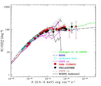
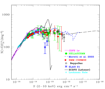
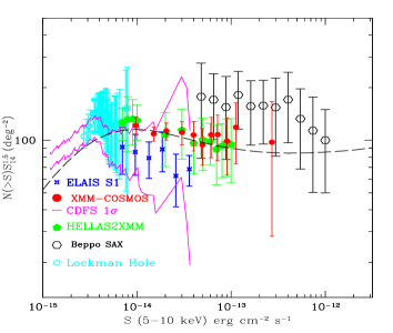
Figure 1.: The X-ray logN-logS compared to the survey listed in the labels in the 0.5–2 keV, 2–10 keV and 5–10 keV energy bands, respectively $Top~{}Left,~{}Top~{}Right~{}and~{}Bottom~{}Left~{}Panels$. The $black-dashed$ line represents the prediction of Gilli, Comastri & Hasinger (2006). $Bottom~{}Right~{}Panel:$ The counts in cell fluctuations within the XMM-COSMOS field on different angular scales. The dashed lines represent the 1$\sigma$ expected fluctuation.

The amplitude of source counts distributions varies significantly among different surveys (see e.g. Yang et al. 2003; Cappelluti et al. 2005, and references therein). This ”sample variance”, can be explained and predicted as a combination of Poissonian variations and effects due to the clustering of sources (Peebles 1980; Yang et al. 2003). In order to determine whether the differences observed in the source counts of different surveys could arise from the clustering of X-ray sources, we estimated the amplitude of the fluctuations from our data, by producing subsamples of our survey with areas comparable to those of. e.g., Chandra surveys.
The XMM-COSMOS field and the Monte Carlo sample fields of Section 4 were divided in 4,9,16 and 25 square boxes. Making use of the 0.5–2 keV energy band data, we computed for each subfield, the ratio of the number of real sources to the number of random source. Both the random and the real sample were cut to a flux limit of 5$\times$10^-15 erg cm^-2 s^-1. In the lower right panel of Figure 1 we plot the ratio of the data to the random sample as a function of the size of the cells under investigation. The predicted fractional standard deviations are 0.13, 0.19, 0.23 and 0.28 on scales of 0.44 deg², 0.19 deg², 0.11 deg² and 0.07 deg², respectively. The measure fractional standard deviations are 0.09, 0.20, 0.21 and 0.24 on the same scales, respectively. The ratio of the clusting to the Poissonian variance is expected to scale as $\sigma_{cl}/\sigma_{p}\propto\mathcal{N}^{0.5}\theta_{0}^{(\gamma-1)/2}a^{(3-\gamma)/2}$. We therefore conclude that at this scales and at fluxes sampled here the major contribution to source counts fluctuations is due to Poissonian noise. This analysis is at least qualitatively consistent with Figure 2, which shows a significantly larger dispersion in the data from different surveys in the hard band than in the soft band. Moreover, the results here discussed are also consistent with the observed fluctuations in the deep Chandra fields (see, for example, Bauer et al. 2004). Large area, moderately deep surveys like XMM-COSMOS are needed to overcome the problem of low counting statistics, typical of deep pencil beam surveys, and, at the same time, to provide a robust estimate of the effect of large scale structure on observed source counts.

Acknowledgments.

This work is based on observations obtained with XMM–Newton , an ESA science mission with instruments and contributions directly funded by ESA Member States and NASA; also based on data collected at the Canada-France-Hawaii Telescope operated by the National Research Council of Canada, the Centre National de la Recherche Scientifique de France and the University of Hawaii.

References

- Bauer et al. (2004) Bauer, F. E., Alexander, D. M., Brandt, W. N., Schneider, D. P., Treister, E., Hornschemeier, A. E., & Garmire, G. P. 2004, AJ, 128, 2048
- Cappelluti et al. (2005) Cappelluti, N., Cappi, M., Dadina, M., Malaguti, G., Branchesi, M., D’Elia, V., & Palumbo, G. G. C. 2005, A&A, 430, 39
- Cappelluti et al. (2007) Cappelluti, N., et al 2007, ApJSin press, ArXiv Astrophysics e-prints, arXiv:astro-ph/0701196
- Della Ceca et al. (2004) Della Ceca, R., et al. 2004, A&A, 428, 383
- Fiore et al. (2003) Fiore, F., et al. 2003, A&A, 409, 79
- Giacconi et al. (2001) Giacconi, R., et al. 2001, ApJ, 551, 624
- Gilli, Comastri & Hasinger (2006) Gilli, R., Comastri, A. & Hasinger, G. 2006, A&A, in press, astro-ph/0610939
- Giommi et al. (2000) Giommi, P., Perri, M., & Fiore, F. 2000, A&A, 362, 799
- Green et al. (2004) Green, P. J., et al. 2004, ApJS, 150, 43
- Hasinger et al. (1993) Hasinger, G., Burg, R., Giacconi, R., Hartner, G., Schmidt, M., Trumper, J., & Zamorani, G. 1993, A&A, 275, 1
- Hasinger et al. (2006) Hasinger, G. et al. 2006, ApJSin press, ArXiv Astrophysics e-prints, arXiv:astro-ph/0612311
- Lehmer et al. (2005) Lehmer, B. D., et al. 2005, ApJS, 161, 21
- Kim et al. (2004) Kim, D.-W., et al. 2004, ApJ, 600, 59
- Murray et al. (2005) Murray, S. S., et al. 2005, ApJS, 161, 1
- Nandra et al. (2005) Nandra, K., et al. 2005, MNRAS, 356, 568
- Peebles (1980) Peebles, P. J. E. 1980, The large-scale structure of the universe (Princeton, N.J., Princeton University Press)
- Puccetti et al. (2006) Puccetti et al. 2006, A&A, 457, 501
- Scoville et al. (2006) Scoville, N.Z. et al., 2007, ApJSin press, 2006, ArXiv Astrophysics e-prints, arXiv:astro-ph/0612305
- Ueda et al. (1999) Ueda, Y., et al. 1999, ApJ, 518, 656
- Virani et al. (2006) Virani, S. N., Treister, E., Urry, C. M., & Gawiser, E. 2006, AJ, 131, 2373
- Yang et al. (2003) Yang, Y., Mushotzky, R. F., Barger, A. J., Cowie, L. L., Sanders, D. B., & Steffen, A. T. 2003, ApJ, 585, L85