The Einstein relation generalized to non-equilibrium

Abstract

The Einstein relation connecting the diffusion constant and the mobility is violated beyond the linear response regime. For a colloidal particle driven along a periodic potential imposed by laser traps, we test the recent theoretical generalization of the Einstein relation to the non-equilibrium regime which involves an integral over measurable velocity correlation functions.

A comprehensive theory of systems driven out of equilibrium is still lacking quite in contrast to the universal description of equilibrium systems by the Gibbs-Boltzmann distribution. Linear response theory provides exact relations valid, however, only for small deviations from equilibrium Kubo et al. (1991). The arguably most famous linear response relation is the Einstein relation

$$D=k_{\mathrm{B}}T\mu,$$ (1)

involving the diffusion constant $D$, the mobility $\mu$, and the thermal energy $k_{\mathrm{B}}T$ Einstein (1905). In his original derivation for a suspension in a force field, Einstein balances the diffusive current with a linear drift. The Einstein relation embodies a deep connection between fluctuations causing diffusion and dissipation responsible for friction expressed by a finite mobility.

In the present Letter, we report on the extension of the classical Einstein relation beyond the linear response regime using a driven colloidal particle as a paradigmatic system. Our previous theoretical work Speck and Seifert (2006) and its present experimental test thus introduce a third type of exact relation valid for and relevant to small driven systems coupled to a heat bath of constant temperature $T$. The previously discovered exact relations comprise, first, the fluctuation theorem Evans et al. (1993); Gallavotti and Cohen (1995) which quantifies the steady state probability of observing trajectories of negative entropy production. Second, the Jarzynski relation Jarzynski (1997) expresses the free energy difference between different equilibrium states by a nonlinear average of the work spent in driving such a transition Bustamante et al. (2005). Both the fluctuation theorem and the Jarzynski relation as well as their theoretical extensions Crooks (2000); Hatano and Sasa (2001); Seifert (2005) have been tested in various experimental systems such as micro-mechanically manipulated biomolecules Liphardt et al. (2002); Collin et al. (2005), colloids in time-dependent laser traps Wang et al. (2002); Blickle et al. (2006); Trepagnier et al. (2004), Rayleigh-Benard convection Ciliberto and Laroche (1998), mechanical oscillators Douarche et al. (2005), and optically driven single two-level systems Schuler et al. (2005). Such exact relations (and the study of their limitations) are fundamentally important since they provide the first elements of a future more comprehensive theory of non-equilibrium systems.

For a non-equilibrium extension of the Einstein relation (1), consider the overdamped motion $x(t)$ of a particle moving along a periodic one-dimensional potential $V(x)$ governed by the Langevin equation

$$\dot{x}(t)=\frac{1}{\gamma}F(x(t))+\xi(t)$$ (2)

with $F=-\partial V/\partial x+f$ and $f$ a non-conservative force. The friction coefficient $\gamma$ determines the correlations $\langle\xi(t)\xi(t^{\prime})\rangle=2(k_{\mathrm{B}}T/\gamma)\delta(t-t^{\prime})$ of the white noise $\xi$. Therefore Eq. (2) describes a colloidal bead driven to non-equilibrium under the assumption that the fluctuating forces arising from the heat bath are not affected by the driving.

For the crucial quantities $D$ and $\mu$, it is convenient to adapt definitions which can be used both in equilibrium and beyond linear response, i.e., in a non-equilibrium steady state characterized by $f=\text{const.}\neq 0$. The diffusion coefficient is given by

$$D=\lim_{t\to\infty}\,[\langle x^{2}(t)\rangle-\langle x(t)\rangle^{2}]/(2t),$$ (3)

where $\langle\cdots\rangle$ denotes the ensemble average. Both theoretical work Reimann et al. (2001) and a recent experiment Lee and Grier (2006) have shown that the force-dependent diffusion constant can be substantially larger than its equilibrium value. The mobility

$$\mu=\frac{\partial\langle\dot{x}\rangle}{\partial f}$$ (4)

quantifies the response of the mean velocity $\langle\dot{x}\rangle$ to a small change of the external force $f$. If the response is taken at $f=0$, which corresponds to equilibrium, one has the linear response relation (1). How does the Einstein relation change for $f\neq 0$, i.e., what is the relation between a force-dependent diffusion constant $D(f)$ and a force-dependent mobility $\mu(f)$? Is there a simple relation at all? We have recently shown that under non-equilibrium conditions the Einstein relation (1) has to be replaced by Speck and Seifert (2006)

$$D=k_{\mathrm{B}}T\mu+\int_{0}^{\infty}\mathrm{d}\tau\;I(\tau),$$ (5)

where the second term on the right hand side is given by an integral over a known “violation function” $I(\tau)$ involving measurable velocity correlations to be discussed in detail below. Such a relation is complementary to introducing an effective temperature which replaces $T$ in Eq. (1) in an attempt to keep its simple form Crisanti and Ritort (2003); Hayashi and Sasa (2004). It has the advantage that knowledge of $I(\tau)$ offers us a better understanding of the crucial characteristics of the non-equilibrium steady state that causes the breakdown of the Einstein relation (1).

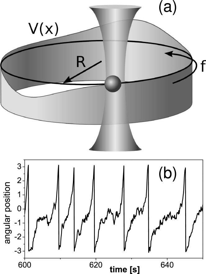
Figure 1: (a) Experimental setup. (b) Typical trajectory of the angular particle position for a mean particle revolution time $\simeq 5.8\;\mathrm{s}$.

In our experiment we subject a single colloidal silica bead with $1.85\;\mathrm{\mu m}$ diameter to a non-equilibrium steady state by forcing it along a toroidal trap ($R=1.75\;\mathrm{\mu m}$) created by tightly focussed rotating optical tweezers  Faucheux et al. (1995); Lutz et al. (2006) (see Fig. 1). This is achieved by focusing the beam of a Nd:YAG laser ($\lambda=532\;\mathrm{nm}$) with a microscope objective (100x, NA=1.3) into a sample cell containing a highly diluted aqueous suspension of silica particles with $1.85\;\mathrm{\mu m}$ diameter. A pair of galvanometric driven mirrors with telescope optics deflects the beam along a circular path and thus confines the silica bead to an effectively one-dimensional motion. Depending on the velocity of the rotating trap three different regimes can be distinguished Faucheux et al. (1995). (i) For small velocities friction forces are much smaller than the trapping force, the trapped particle is able to follow the trap. (ii) With increasing velocity the trap is not strong enough to compensate the viscous force of the fluid, the particle escapes from the laser trap. However, every time the laser passes the particle it is still dragged a small distance along the circle and moves with a constant mean velocity around the torus. (iii) As the focus speed increases (quasi)-equilibrium conditions are established and the particle is able to diffuse freely along the torus. With the trap rotation frequency set to $567\;\mathrm{Hz}$ the experiments are performed in the intermediate regime (ii) where the particle is observed to circulate with a constant mean velocity. Since the displacement of the particle by a single kick depends on the laser intensity and is approximately $10\;\mathrm{nm}$, under our experimental conditions the spatial ($50\;\mathrm{nm}$) and temporal ($80\;\mathrm{ms}$) resolution of digital video microscopy is not sufficient to resolve single ”kicking” events. Therefore the particle can be considered to be subjected to a constant force $f$ along the angular direction $x$. Additionally the scanning motion is synchronized with an electro-optical modulator (EOM) which allows the periodic variation of the laser intensity along the toroid. In the experiment the tweezers intensity $P$ is weakly modulated ($\Delta P/P\leq 10\%$). This small intensity modulation superimposes an additional periodic potential $V(x)$ acting on the particle when moving along the torus. As the result, the particle moves in a tilted periodic potential. Both the potential $V(x)$ and the driving force $f$ are not known from the input values to the EOM but must be reconstructed as described in detail below.

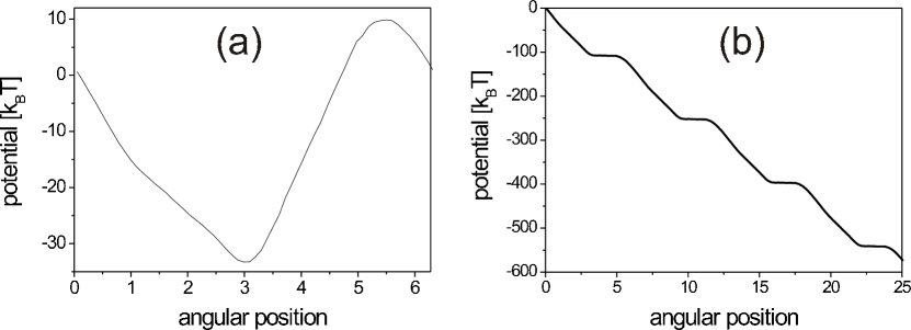
Figure 2: (a) Reconstructed potential $V(x)$. (b) Tilted potential. The colloidal particle is subjected to a constant driving force $f\simeq 0.06\;\mathrm{pN}$ and the periodic potential $V(x)$.

The central quantitity of Eq. (5) is the violation function $I(\tau)$ which can be written as Speck and Seifert (2006)

$$I(\tau)=\langle[\dot{x}(t+\tau)-\langle\dot{x}\rangle][v_{\mathrm{s}}(x(t))-\langle\dot{x}\rangle]\rangle.$$ (6)

It correlates the actual velocity $\dot{x}(t)$ with the local mean velocity $v_{\mathrm{s}}(x)$ subtracting from both the global mean velocity $\langle\dot{x}\rangle=2\pi Rj_{\mathrm{s}}$ that is given by the net particle flux $j_{\mathrm{s}}$ through the torus. In one dimension for a steady state, the current must be the same everywhere and hence $j_{\mathrm{s}}$ is a constant. The offset $t$ is arbitrary because of time-translational invariance in a steady state and in the following we set $t=0$. The local mean velocity $v_{\mathrm{s}}(x)$ is the average of the stochastic velocity $\dot{x}$ over the subset of trajectories passing through $x$. An equivalent expression is $j_{\mathrm{s}}=v_{\mathrm{s}}(x)p_{\mathrm{s}}(x)$ connecting the current with the probability density $p_{\mathrm{s}}(x)$. The local mean velocity can thus be regarded as a measure of the local violation of detailed balance. Since in equilibrium detailed balance holds and therefore $v_{\mathrm{s}}(x)=\langle\dot{x}\rangle=0$, the violation (6) vanishes and Eq. (5) reduces to Eq. (1).

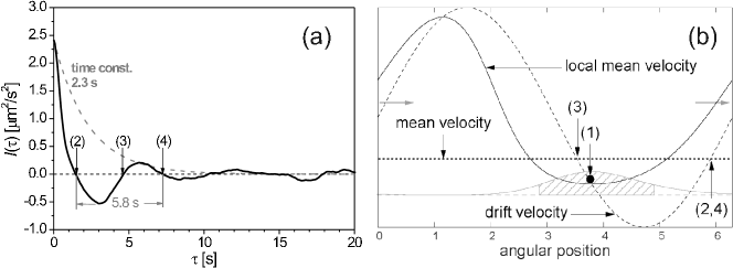
Figure 3: a) Experimentally measured violation function $I(\tau)$ (solid line). b) Comparison of the velocities involved in the violation function $I(\tau)$. For an ideal cosine potential, we sketch the probability distribution $p_{\mathrm{s}}(x)$ (solid gray line), the local mean velocity $v_{\mathrm{s}}(x)$ together with the drift velocity and their mean $\langle\dot{x}\rangle$ versus the angular particle position. The drift velocity is the deterministic part $F/\gamma$ of the actual velocity $\dot{x}$. The sign change in $I(\tau)$ at (2), (3), and (4) can be understood as follows. In a steady state, a single particle trajectory will start with highest probability in the shaded region and, for an illustration, we choose its maximum as starting point (1) determining the value $v_{\mathrm{s}}(x(t))$ in Eq. (6). Neglecting thermal fluctuations, the particle would follow the dashed line and during a small time step $\tau$ the product $F(x(t+\tau))v_{\mathrm{s}}(x(t))$ is positive. If the particle passes (2), the product would become negative. The sign changes again if the particle passes (3) and then (4) and so on due to the periodic nature of the potential. Thermal noise and averaging over all trajectories does not change this behavior responsible for the oscillations of $I(\tau)$.

For an experimental test of the non-equilibrium Einstein relation (5), we measure trajectories of a single colloidal particle for different driving forces $f$ by adjusting the intensity transmitted through the EOM. From a linear fit to the data we first determine the mean global velocity $\langle\dot{x}\rangle$. Next, we extract the mean local velocity $v_{\mathrm{s}}(x)$ from the histogram $p_{\mathrm{s}}(x)$ with the coordinate $x$ confined to $0\leq x\leq 2\pi R$. Since measurements are performed with a sampling rate of $80\;\mathrm{ms}$, we cannot directly access the velocity $\dot{x}(t)$ experimentally. To calculate the violation integral $I(\tau)$, we decompose $\dot{x}(t)$ into a randomly fluctuating Brownian part and a drift term, see Eq. (2). We then transform $I(\tau)$ as

$$\begin{split}I(\tau)=&\langle[v_{\mathrm{s}}(x(\tau))-\frac{k_{\mathrm{B}}T}{\gamma}\frac{\partial\Phi}{\partial x}(x(\tau))]v_{\mathrm{s}}(x(0))\rangle-\langle\dot{x}\rangle^{2}\\ &+\langle\xi(\tau)v_{\mathrm{s}}(x(0))\rangle.\end{split}$$ (7)

The generalized potential $\Phi(x)$ is determined via the measured stationary probability distribution, $p_{\mathrm{s}}(x)=\exp[-\Phi(x)]$ Speck and Seifert (2006). For $\tau>0$, the last term vanishes because then $\xi(t+\tau)$ and $x(t)$ are uncorrelated. Thus the function $I(\tau)$ depends on two measurable quantities, the current $j_{\mathrm{s}}$ and the stationary probability distribution $p_{\mathrm{s}}(x)$.

The potential $V$ and the driving force $f$ are determined by integrating the force

$$F=-\frac{\partial V}{\partial x}+f=\gamma v_{\mathrm{s}}-k_{\mathrm{B}}T\frac{\partial\Phi}{\partial x}$$ (8)

along the torus. We obtain

$$f=\frac{\gamma}{2\pi R}\int_{0}^{2\pi R}\mathrm{d}x\;v_{\mathrm{s}}(x)$$ (9)

and

$$V(x)=k_{\mathrm{B}}T\Phi(x)+\int_{0}^{x}\mathrm{d}x^{\prime}\;[f-\gamma v_{\mathrm{s}}(x^{\prime})]$$ (10)

up to an irrelevant constant. In Eq. (9), terms involving $V$ and $\Phi$ are zero due to the periodicity of our system. Both, the potential $V(x)$ and the tilted potential $V(x)-fx$ are shown in Fig. 2. The mobility $\mu=\Delta\langle\dot{x}\rangle/\Delta f$ is determined from the change of the global mean velocity $\Delta\langle\dot{x}\rangle$ upon a small variation of the force $\Delta f$.

With the experimentally determined quantities, we measure the violation function $I(\tau)$ shown as solid line in Fig. 3a for $f=0.06\;\mathrm{pN}$. It clearly displays the two time scales present in the system. First, the driving leads to an oscillatory behavior with a period equal to the mean revolution time $\simeq 5.8\;\mathrm{s}$. Second, the diffusion causes a broadening of the particle’s position resulting in a decorrelation between actual and local velocity and hence an exponential decay with time constant $\simeq 2.3\;\mathrm{s}$ indicated by the dashed line (Fig. 3a). To understand the behavior of $I(\tau)$ in more detail it is helpful to compare the different velocities involved in the violation function $I(\tau)$ which are sketched in Fig. 3b.

After numerical integration of the experimentally determined $I(\tau)$ we finally calculate the diffusion coefficient according to Eq. (5). To quantify the relative importance of the violation integral we plot the two terms of the right hand side of Eq. (5) separately for five different values of the driving force in Fig. 4. Their sum is in good agreement with the independently measured diffusion coefficient directly obtained from the particles trajectory using Eq. (3). As the maximal error for the independent measurements we estimated from our data $\pm 3\%$ for the diffusion coefficient $D$, up to $\pm 10\%$ for the violation integral, and $\pm 7\%$ for the mobility $\mu$.

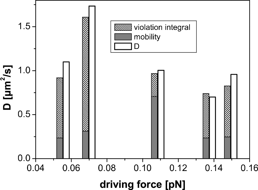
Figure 4: Experimental test of Eq. (5) for different driving forces $f$. The open bars show the measured diffusion coefficients $D$. The stacked bars are mobility (gray bar) and integrated violation (hatched bar), respectively.

We emphasize that under our experimental parameters the violation term dominates the diffusion coefficient (up to $80\%$) and must not be ignored. In Fig. 4 one observes a non-monotonic dependence of the violation integral on the driving force. This is due to the fact that the maxima of $\mu(f)$ and $D(f)$ do not occur at the same driving force but are slightly offset Reimann et al. (2001). This implies for the violation function a maximum followed by a minimum as a function of $f$. For very small driving forces, the bead is close to equilibrium and its motion can be described using linear response theory. As a result, the violation integral is negligible. Experimentally, this regime is difficult to access since $D$ and $\mu$ become exponentially small and cannot be measured at reasonable time scales for small forces and potentials as deep as $40\,k_{\mathrm{B}}T$ (cf. Fig. 2a). For much larger forces, the relative magnitude of the violation term becomes smaller as well. In this limit, the imposed potential becomes irrelevant and the spatial dependence of the local mean velocity, which is the source of the violation term, vanishes. The fact that in our regime the violation term is of the same order of magnitude as the mobility proves that we are indeed probing the regime beyond linear response. Still, the description of the colloidal motion by a Markovian (memory-less) Brownian motion with drift as implicit in our analysis remains obviously a faithful representation since the theoretical results are derived from such a framework.

The Einstein relation generalized to non-equilibrium as presented and tested here for the driven motion along a single coordinate could be considered as a paradigm. Extending such an approach to interacting particles and resolving frequency dependent versions of Eq. (6) Speck and Seifert (2006) while certainly experimentally challenging will provide further insight into crucial elements of a future systematic theory of non-equilibrium systems.

References

- Kubo et al. (1991) R. Kubo, M. Toda, and N. Hashitsume, Statistical Physics II (Springer-Verlag, Berlin, 1991), 2nd ed.
- Einstein (1905) A. Einstein, Ann. Phys. 17, 549 (1905).
- Speck and Seifert (2006) T. Speck and U. Seifert, Europhys. Lett. 74, 391 (2006).
- Evans et al. (1993) D. J. Evans, E. G. D. Cohen, and G. P. Morriss, Phys. Rev. Lett. 71, 2401 (1993).
- Gallavotti and Cohen (1995) G. Gallavotti and E. G. D. Cohen, Phys. Rev. Lett. 74, 2694 (1995).
- Jarzynski (1997) C. Jarzynski, Phys. Rev. Lett. 78, 2690 (1997).
- Bustamante et al. (2005) C. Bustamante, J. Liphardt, and F. Ritort, Physics Today 58, 43 (2005).
- Crooks (2000) G. E. Crooks, Phys. Rev. E 61, 2361 (2000).
- Hatano and Sasa (2001) T. Hatano and S. Sasa, Phys. Rev. Lett. 86, 3463 (2001).
- Seifert (2005) U. Seifert, Phys. Rev. Lett. 95, 040602 (2005).
- Liphardt et al. (2002) J. Liphardt, S. Dumont, S. B. Smith, I. Tinoco Jr, and C. Bustamante, Science 296, 1832 (2002).
- Collin et al. (2005) D. Collin, F. Ritort, C. Jarzynski, S. Smith, I. Tinoco, and C. Bustamante, Nature 437, 231 (2005).
- Wang et al. (2002) G. M. Wang, E. M. Sevick, E. Mittag, D. J. Searles, and D. J. Evans, Phys. Rev. Lett. 89, 050601 (2002).
- Blickle et al. (2006) V. Blickle, T. Speck, L. Helden, U. Seifert, and C. Bechinger, Phys. Rev. Lett. 96, 070603 (2006).
- Trepagnier et al. (2004) E. H. Trepagnier, C. Jarzynski, F. Ritort, G. E. Crooks, C. J. Bustamante, and J. Liphardt, Proc. Natl. Acad. Sci. U.S.A. 101, 15038 (2004).
- Ciliberto and Laroche (1998) S. Ciliberto and C. Laroche, J. Phys. IV France 8 (P6), 215 (1998).
- Douarche et al. (2005) F. Douarche, S. Ciliberto, A. Petrosyan, and I. Rabbiosi, Europhys. Lett. 70, 593 (2005).
- Schuler et al. (2005) S. Schuler, T. Speck, C. Tietz, J. Wrachtrup, and U. Seifert, Phys. Rev. Lett. 94, 180602 (2005).
- Reimann et al. (2001) P. Reimann, C. van den Broeck, H. Linke, P. Hänggi, M. Rubi, and A. Pérez-Madrid, Phys. Rev. Lett. 87, 010602 (2001).
- Lee and Grier (2006) S.-H. Lee and D. G. Grier, Phys. Rev. Lett. 96, 190601 (2006).
- Crisanti and Ritort (2003) A. Crisanti and F. Ritort, J. Phys. A: Math. Gen. 36, R181 (2003).
- Hayashi and Sasa (2004) K. Hayashi and S. Sasa, Phys. Rev. E 69, 066119 (2004).
- Faucheux et al. (1995) L. Faucheux, G. Stolovitzky, and A. Libchaber, Phys. Rev. E 51, 5239 (1995).
- Lutz et al. (2006) C. Lutz, M. Reichert, H. Stark, and C. Bechinger, Europhys. Lett. 74, 719 (2006).