Physics Beyond the Standard Model and Dark Matter
1 Introduction
I’m honored to be invited as a lecturer at a Les Houches summer school which has a great tradition. I remember reading many of the lectures from past summer schools when I was a graduate student and learned a lot from them. I’m also looking forward to have a good time in the midst of beautiful mountains, even though the weather doesn’t seem to be cooperating. I’m not sure if I will ever get to see Mont Blanc!
I was asked to give four general lectures on physics beyond the standard model. This is in some sense an ill-defined assignment, because it is a vast subject for which we know pratically nothing about. It is vast because there are so many possibilities and speculations, and a lot of ink and many many pages of paper had been devoted to explore it. On the other hand, we know practically nothing about it by definition, because if we did, it should be a part of the standard model of particle physics already. I will therefore focus more on the motivation why we should consider physics beyond the standard model and discuss a few candidates, and there is no way I can present all the examples exhaustively. In addition, after reviewing the program, I’ve realized that there are no dedicated lectures on dark matter. Since this is a topic where particle physics and cosmology (I believe) are likely to come together in the near future, it is relevant to the theme of the school “Particle Physics and Cosmology: the Fabric of Spacetime.” Therefore I will emphasize this connection in some detail.
Because I try to be pedagogical in lectures, I will probably discuss many points which some of you already know very well. Given the wide spectrum of background you have, I aim at the common denominator. Hopefully I don’t end up boring you all!
1.1 Particle Physics and Cosmology
At the first sight, it seems crazy to talk about particle physics and cosmology together. Cosmology is the study of the universe, where the distance scale involved is many Gigaparsecs cm. Particle physics studies the fundamental constituent of matter, now reaching the distance scale of cm. How can they have anything in common?
The answer is the Big Bang. Discovery of Hubble expansion showed that the visible universe was much smaller in the past, and the study of cosmic microwave background showed the universe was filled with a hot plasma made of photons, electrons, and nuclei in thermal equilibrium. It was hot. As we contemplate earlier and earlier epochs of the universe, it was correspondingly smaller and hotter.
On the other hand, the study of small scales in particle physics translates to large momentum due to the uncertainty principle, . Since large momentum requires relativity, it also means high energy . Physics at higher energies is relevant for the study of higher temperatures , which was the state of the earlier universe.
This way, Big Bang connects microscopic physics to macroscopic physics. And we have already seen two important examples of this connection.
Atomic and molecular spectroscopy is based on quantum physics at the atomic distance cm. This spectroscopy is central to astronomy to identify the chemical composition of faraway stars and galaxies which we never hope to get to directly and measure their redshifts to understand their motion including the expansion of the space itself. The cosmic microwave background also originates from the atomic-scale physics when the universe was as hot as K and hence was in the plasma state. This is the physics which we believe we understand from the laboratory experiments and knowledge of quantum mechanics and hence we expect to be able to extract interesting information about the universe. Ironically, cosmic microwave background also poses a “wall” because the universe was opaque and we cannot “see” with photons the state of the universe before this point. We have to rely on other kinds of “messengers” to extract information about earlier epochs of the universe.
The next example of the micro-macro connection concerns with nuclear physics. The stars are powered by nuclear fusion, obviously a topic in nuclear physics. This notion is now well tested by the recent fantastic development in the study of solar neutrinos, where the core temperature of the Sun is inferred from the helioseismology and solar neutrinos which agree at better than a percent level. Nuclear physics also determines death of a star. Relatively heavy stars even end up with nuclear matter, i.e. neutron stars, where the entire star basically becomes a few kilometer-scale nucleus. On the other hand, when the universe was as hot as MeV (ten billion degrees Kelvin), it was too hot for protons and neutrons to be bound in nuclei. One can go through theoretical calculations on how the protons and neutrons became bound in light nuclear species, such as deuterium, 3He, 4He, 7Li, based on the laboratory measurements of nuclear fusion cross sections, as well as number of neutrino species from LEP (Large Electron Positron collider at CERN). This process is called Big-Bang Nucleosynthesis (BBN). There is only one remaining free parameter in this calculation: cosmic baryon density. The resulting predictions can be compared to astronomical determinations of light element abundances by carefully selecting the sites which are believed to be not processed by stellar evolutions. There is (in my humble opinion) reasonable agreement between the observation and theoretical predictions (see, e.g., [1]). This agreement gives us confidence that we understand the basic history of the universe since it was as hot as MeV.
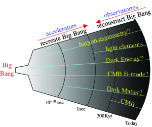
We currently do not have messengers from epochs in early universe above the MeV temperature. In other words, our understanding of early universe physics is not tested well for MeV. Yet many of the topics discussed in this school are possible messengers from earlier era: dark matter ( GeV?), baryon asymmetry of the universe ( GeV?), density perturbations (scalar and tensor components) from the inflationary era ( GeV?). These are the energy scales that laboratory measurements have not reached to reveal the full particle spectrum and their interactions, hence the realm of physics beyond the standard model. Understanding of such early stages of the universe requires the development in particle physics, while the universe as a whole may be regarded as a testing ground of hypothesized particle physics at high energies beyond the reach of accelerators. This way, cosmology and particle physics help and require each other.
1.2 Next Threshold
There is a strong anticipation in the community that we are just about to reveal a new threshold in physics. Let me tell you why from a historical perspective.
We (physicists) do not witness crossing a new threshold very often, but each time it happened, it resulted in a major change in our understanding of Mother Nature.
Around year 1900, we crossed the threshold of atomic scale. It is impressive to recall how much progress chemists have made without knowing the underlying dynamics of atoms and molecules. But the empirical understanding of chemistry had clear limitation. For example, van der Waals equation of state showed there was the distance scale of about cm below which the state-of-art scientific knowledge of the time could not be applied, namely the size of atoms. Once the technology improved to study precision spectroscopy that allowed people to probe physics inside the atoms, a revolution followed. It took about three decades for quantum mechanics to be fully developed but it forever changed our understanding of nature. The revolution went on well into the 40’s when the marriage of quantum mechanics and relativity was completed in Quantum ElectroDynamics.
Next important threshold was crossed around 1950 when new hadron resonances and strange particles were discovered, crossing the threshold of the strong interaction scale cm. Discovery of a zoo of “elementary particles” led to a great deal of confusion for about three decades. It eventually led to the revelation of non-perturbative dynamics of quantum field theory, namely confinement of quarks, dimensional transmutation, and dynamical symmetry breaking of chiral symmetry. More importantly, it showed a new layer in nature where quarks and gluons take over the previous description of subatomic world with protons and neutrons. The experimental verification of this theory, Quantum ChromoDynamics, took well into 90’s at numerous accelerators PETRA, PEP, TRISTAN, LEP, and HERA.
One more force that is yet to be fully understood is the weak interaction. Its scale was known from the time of Fermi back in 1933 when he wrote the first theory of nuclear beta decay. The theory contained one dimensionful constant . Seven decades later, we are just about to reach this energy scale in accelerator experiments, at Tevatron and LHC. We do not really know what Nature has in store for us, but at least we’ve known all along that this is another important energy scale in physics. If we are not misled, this is the energy scale associated with the cosmic superconductor. Just like the Meissner effect lets magnetic field penetrate into a superconductor only over a finite distance, the cosmic superconductor lets the weak force carried by and bosons go over a tiny distance: a billionth of a nanometer. Right now we are only speculating what revolution may take place at this distance scale. A new layer of matter? New dimensions of space? Quantum dimensions? Maybe string theory? We just don’t know yet.
Of course historical perspective does not guarantee that history repeats itself in an equally exciting fashion. But from all what we know, there is a good reason to think that indeed a new threshold is waiting to be discovered at the TeV energy scale, as I will discuss in the next section. Another simple fact is that crossing a new threshold is something like twice-in-a-century experience. I’m excited to think that we are just about to witness one, a historic moment.
An interesting question is what fundamental physics determines these thresholds. The atomic scale, that looked like a fundamental limitation in understanding back in the 19th century, did not turn out to be a fundamental scale at all. It is a derived scale from the mass of the electron and the fundamental constants,
| (1.1) |
The strong-interaction scale is also a derived energy scale from the coupling constant
| (1.2) |
where is the strong coupling constant defined at a high-energy scale and is the beta function coefficient. Because of the asymptotic freedom, the strong coupling constant is weak (what an oxymoron!) at high energies, while it becomes infinitely strong at low energies. The scale of strong interaction is where the strength of the interaction blows up. In other words, the two thresholds we have crossed so far were extremely exciting, yet they turned out to be not fundamental! They point to yet deeper physics that determine these parameters in nature. Maybe the weak-interaction scale is also a derived scale from some deeper physics at yet shorter distances.
2 Why Beyond the Standard Model
2.1 Empirical Reasons
Until about ten years ago, particle physicists lamented that the standard model described every new data that came out from experiments and we didn’t have a clue what may lie beyond the standard model. Much of the discussions on physics beyond the standard model therefore were not based on data, but rather on theoretical arguments, primarily philosophical and aesthetic displeasure with the standard model. It all changed the last ten years when empirical evidence appeared that demonstrated that the standard model is incomplete:
-
•
Non-baryonic dark matter,
-
•
Dark energy,
-
•
Neutrino mass,
-
•
Nearly scale-invariant, Gaussian, and apparently acausal density perturbations,
-
•
Baryon asymmetry.
I will discuss strong evidence for non-baryonic dark matter and dark matter later in my lectures. Density fluctuation is covered in many other lectures in this school by Lev Kofman, Sabino Matarrese, Yannick Mellier, Simon Prunet, and Romain Teyssier. Neutrino mass is discussed by Sergio Pastor, and baryon asymmetry by Jim Cline. The bottom line is simple: we already know that there must be physics beyond the standard model. However, we don’t necessarily know the energy (or distance) scale for this new physics, nor what form it takes. One conservative approach is to try to accommodate all of these established empirical facts into the standard model with minimum particle content: The New Minimal Standard Model [2]. I will discuss some aspects of the model later. But theoretical arguments suggest the true model be much bigger, richer, and more interesting.
2.2 Philosophical and Aesthetic Reasons
What are the theoretical arguments that demand physics beyond the standard model? As I mentioned already, they are based on somewhat philosophical arguments and aesthetic desires and not exactly on firm footing. Nonetheless they are useful and suggestive, especially because nature did solve some of the similar problems in the past by invoking interesting mechanisms. A partial list relevant to my lectures here is
-
•
Hierarchy problem: why ?
-
•
Why ?
-
•
Why are there three generations of particles?
-
•
Why are the quantum numbers of particles so strange, yet do anomalies cancel so non-trivially?
For an expanded list of the “big questions”, see e.g., [3].
To understand what these questions are about, it is useful to remind ourselves how the standard model works. It is a gauge theory based on the gauge group with the Lagrangian
It looks compact enough that it should fit on a T-shirt.111It reminds me of an anecdote from when the standard model was just about getting off the ground around 1978. There was a convergence of the data to the standard model and people got very excited about it. Then Tini Veltman gave a talk asking “do you really think this is great model?” and wrote down every single term in the Lagrangian without using a compact notation used here over pages and pages of transparencies. Unfortunately I don’t remember who told me this story. Why don’t we see such a T-shirt while we see Maxwell equations a lot?
The first two lines describe the gauge interactions. The covariant derivatives in the second line are determined by the gauge quantum numbers given in this table:
| chirality | ||||||||
| 3 | 2 | left | ||||||
| 3 | 1 | right | ||||||
| 3 | 1 | right | ||||||
| 1 | 2 | left | ||||||
| 1 | 1 | right | ||||||
This part of the Lagrangian is well tested, especially by the LEP/SLC data in the 90’s. However, the quantum number assignments (especially hypercharges) appear very strange and actually hard to remember.222I often told my friends that I chose physics over chemistry or biology because I didn’t want to memorize anything, but this kind of table casts serious doubt on my choice! Why this peculiar assignment is one of the things people don’t like about the standard model. In addition, they are subject to non-trivial anomaly cancellation conditions for , , , , and Witten’s anomalies. Many of us are left with the feeling that there must be a deep reason for this baroque quantum number assignments which had led to the idea of grand unification.
The third line of the Lagrangian comes with the generation index and is responsible for masses and mixings of quarks and masses of charged leptons. The quark part has been tested precisely in this decade at -factories while there is a glaring omission of neutrino masses and mixings that became established since 1998. In addition, it appears unnecessary for nature to repeat elementary particles three times. The repetition of generations and the origin of mass and mixing patterns remains an unexplained mystery in the standard model.
The last line is completely untested. The first two terms describe the Higgs field and its interaction to the gauge fields and itself. Having not seen the Higgs boson so far, it is far from established. The mere presence of the Higgs field poses an aesthetic problem. It is the only spinless field in the model, but it is introduced for the purpose of doing the most important job in the model. In addition, we have not seen any elementary spinless particle in nature! Moreover, the potential needs to be chosen with to cause the cosmic superconductivity which does not give any reason why our universe is in this state. I will discuss more problems about it in a few minutes. Overall, this part of the model looks very artificial.
The last term is the so-called -term in QCD and violates and . The vacuum angle is periodic under , and hence a “natural” value of is believed to be order unity. On the other hand, the most recent experimental upper limit on the neutron electric dipole moment (90% CL) [4]333This is an amazing limit. If you blow up the neutron to the size of the Earth, this limit corresponds to a possible displacement of an electron by less than ten microns. translates to a stringent upper limit using the formula in [5]. Why is so much smaller than the “natural” value is the strong CP problem, and again the standard model does not offer any explanations.
Now we have more to say about the Higgs sector (the third line). Clearly it is very important because (1) this is the only part of the Standard Model which has a dimensionful parameter and hence sets the overall energy scale for the model, and (2) it has the effect of causing cosmic superconductivity without explaining its microscopic mechanism. For the usual superconductors studied in the laboratory, we can use the same Lagrangian, but it is derived from the more fundamental theory by Bardeen, Cooper, and Schrieffer. The weak attractive force between electrons by the phonon exchange causes electrons to get bound and condense. The “Higgs” field is the Cooper pair of electrons. And one can show why it has this particular potential. In the standard model, we do not know if Higgs field is elementary or if it is made of something else, nor what mechanism causes it to have this potential.
All the puzzles raised here (and more) cry out for a more fundamental theory underlying the Standard Model. What history suggests is that the fundamental theory lies always at shorter distances than the distance scale of the problem. For instance, the equation of state of the ideal gas was found to be a simple consequence of the statistical mechanics of free molecules. The van der Waals equation, which describes the deviation from the ideal one, was the consequence of the finite size of molecules and their interactions. Mendeleev’s periodic table of chemical elements was understood in terms of the bound electronic states, Pauli exclusion principle and spin. The existence of varieties of nuclide was due to the composite nature of nuclei made of protons and neutrons. The list could go on and on. Indeed, seeking answers at more and more fundamental level is the heart of the physical science, namely the reductionist approach.
The distance scale of the Standard Model is given by the size of the Higgs boson condensate GeV. In natural units, it gives the distance scale of cm. We therefore would like to study physics at distance scales shorter than this eventually, and try to answer puzzles whose partial list was given in the previous section.
Then the idea must be that we imagine the Standard Model to be valid down to a distance scale shorter than , and then new physics will appear which will take over the Standard Model. But applying the Standard Model to a distance scale shorter than poses a serious theoretical problem. In order to make this point clear, we first describe a related problem in the classical electromagnetism, and then discuss the case of the Standard Model later along the same line [9].
2.3 Positron Analogue
In the classical electromagnetism, the only dynamical degrees of freedom are electrons, electric fields, and magnetic fields. When an electron is present in the vacuum, there is a Coulomb electric field around it, which has the energy of
| (2.2) |
Here, is the “size” of the electron introduced to cutoff the divergent Coulomb self-energy. Since this Coulomb self-energy is there for every electron, it has to be considered to be a part of the electron rest energy. Therefore, the mass of the electron receives an additional contribution due to the Coulomb self-energy:
| (2.3) |
Experimentally, we know that the “size” of the electron is small, cm. This implies that the self-energy is greater than 10 GeV or so, and hence the “bare” electron mass must be negative to obtain the observed mass of the electron, with a fine cancellation like444Do you recognize ?
| (2.4) |
Even setting a conceptual problem with a negative mass electron aside, such a fine-cancellation between the “bare” mass of the electron and the Coulomb self-energy appears ridiculous. In order for such a cancellation to be absent, we conclude that the classical electromagnetism cannot be applied to distance scales shorter than cm. This is a long distance in the present-day particle physics’ standard.


The resolution to this problem came from the discovery of the anti-particle of the electron, the positron, or in other words by doubling the degrees of freedom in the theory. The Coulomb self-energy discussed above can be depicted by a diagram Fig. 2 where the electron emits the Coulomb field (a virtual photon) which is absorbed later by the electron (the electron “feels” its own Coulomb field).555The diagrams Figs. 2, 4 are not Feynman diagrams, but diagrams in the old-fashioned perturbation theory with different -orderings shown as separate diagrams. The Feynman diagram for the self-energy is the same as Fig. 2, but represents the sum of Figs. 2, 4 and hence the linear divergence is already cancelled within it. That is why we normally do not hear/read about linearly divergent self-energy diagrams in the context of field theory. But now that we know that the positron exists (thanks to Anderson back in 1932), and we also know that the world is quantum mechanical, one should think about the fluctuation of the “vacuum” where the vacuum produces a pair of an electron and a positron out of nothing together with a photon, within the time allowed by the energy-time uncertainty principle (Fig. 3). This is a new phenomenon which didn’t exist in the classical electrodynamics, and modifies physics below the distance scale cm. Therefore, the classical electrodynamics actually did have a finite applicability only down to this distance scale, much earlier than cm as exhibited by the problem of the fine cancellation above. Given this vacuum fluctuation process, one should also consider a process where the electron sitting in the vacuum by chance annihilates with the positron and the photon in the vacuum fluctuation, and the electron which used to be a part of the fluctuation remains instead as a real electron (Fig. 4). V. Weisskopf [10] calculated this contribution to the electron self-energy, and found that it is negative and cancels the leading piece in the Coulomb self-energy exactly:666An earlier paper by Weisskopf actually found two contributions to add up. After Furry pointed out a sign mistake, he published an errata with no linear divergence. I thank Howie Haber for letting me know.
| (2.5) |
After the linearly divergent piece is canceled, the leading contribution in the limit is given by
| (2.6) |
There are two important things to be said about this formula. First, the correction is proportional to the electron mass and hence the total mass is proportional to the “bare” mass of the electron,
| (2.7) |
Therefore, we are talking about the “percentage” of the correction, rather than a huge additive constant. Second, the correction depends only logarithmically on the “size” of the electron. As a result, the correction is only a 9% increase in the mass even for an electron as small as the Planck distance cm.
The fact that the correction is proportional to the “bare” mass is a consequence of a new symmetry present in the theory with the antiparticle (the positron): the chiral symmetry. In the limit of the exact chiral symmetry, the electron is massless and the symmetry protects the electron from acquiring a mass from self-energy corrections. The finite mass of the electron breaks the chiral symmetry explicitly, and because the self-energy correction should vanish in the chiral symmetric limit (zero mass electron), the correction is proportional to the electron mass. Therefore, the doubling of the degrees of freedom and the cancellation of the power divergences lead to a sensible theory of electron applicable to very short distance scales.
2.4 Hierarchy Problem
In the Standard Model, the Higgs potential is given by
| (2.8) |
where . Because perturbative unitarity requires that , is of the order of . However, the mass squared parameter of the Higgs doublet receives a quadratically divergent contribution from its self-energy corrections. For instance, the process where the Higgs doublets splits into a pair of top quarks and come back to the Higgs boson gives the self-energy correction
| (2.9) |
where is the “size” of the Higgs boson, and is the top quark Yukawa coupling. Based on the same argument in the previous section, this makes the Standard Model not applicable below the distance scale of cm. This is the hierarchy problem. In other words, if we don’t solve this problem, we can’t even talk about physics at much shorter distances without an excessive fine-tuning in parameters.
It is worth pondering if the mother nature may fine-tune. Now that the cosmological constant appears to be fine-tuned at the level of , should we be really worried about the fine-tuning of [6]? In fact, some people argued that the hierarchy exists because intelligent life cannot exist otherwise [7]. On the other hand, a different way of varying the hierarchy does seem to support stellar burning and life [8]. I don’t get into this debate here, but I’d like to just point out that a different fine-tuning problem in cosmology, horizon and flatness problems, pointed to the theory of inflation, which in turn appears to be empirically supported by data. I just hope that proper solutions will be found to both of these fine-tuning problems and we will see their manifestations at the relevant energy scale, namely TeV. You have to be an optimist to work on big problems.
3 Examples of Physics Beyond the Standard Model
Given various problems in the standard model discussed in the previous section, especially the hierarchy problem, many possible directions of physics beyond the standard model have been proposed. I can review only a few of them here given the spacetime constraint. But I especially emphasize the aspect of the models that leads to a (nearly) stable neutral particle as a good dark matter candidate.
3.1 Supersymmetry
The motivation for supersymmetry is to make the Standard Model applicable to much shorter distances so that we can hope that the answers to many of the puzzles in the Standard Model can be given by physics at shorter distance scales [11]. In order to do so, supersymmetry repeats what history did with the positron: doubling the degrees of freedom with an explicitly broken new symmetry. Then the top quark would have a superpartner, the stop,777This is a terrible name, which was originally meant to be “scalar top” or “supersymmetric top.” Some other names are even worse: sup, sstrange, etc. If supersymmetry will be discovered at LHC, we should seriously look for better names for the superparticles, maybe after the names of rich donors. whose loop diagram gives another contribution to the Higgs boson self energy
| (3.1) |
The leading pieces in cancel between the top and stop contributions, and one obtains the correction to be
| (3.2) |
One important difference from the positron case, however, is that the mass of the stop, , is unknown. In order for the to be of the same order of magnitude as the tree-level value , we need to be not too far above the electroweak scale. TeV stop mass is already a fine tuning at the level of a percent. Similar arguments apply to masses of other superpartners that couple directly to the Higgs doublet. This is the so-called naturalness constraint on the superparticle masses (for more quantitative discussions, see papers [12]).
Supersymmetry doubles the number of degrees of freedom in the standard model. For each fermion (quarks and leptons), you introduce a complex scalar field (squarks and sleptons). For each gauge boson, you introduce gaugino, a partner Majorana fermion (a fermion field whose anti-particle is itself). I do not go into technical aspect of how to write a supersymmetric quantum field theory; you should consult some review articles [13, 14].
One important point related to dark matter is the proton longevity. We know from experiments such as SuperKamiokande that proton is very long lived (if not immortal). The life time for the decay mode is longer than years, at least twenty-three orders of magnitude longer than the age of the universe! On the other hand, if you write the most general renormalizable theory with standard model particle content consistent with supersymmetry, it allows for vertices such as and (here are color indices). Then one can draw a Feynman diagram like one in Fig. 5. If the couplings are , and superparticles around TeV, one finds the proton lifetime as short as sec; a little too short!
pdecay {fmfgraph*}(100,40) \fmfstraight\fmflefti3,i2,i1 \fmfrighto3,o2,o1 \fmffermioni1,v1 \fmflabeli1 \fmffermioni2,v1 \fmflabeli2 \fmfscalar,label=v2,v1 \fmffermiono1,v2 \fmflabelo1 \fmffermiono2,v2 \fmflabelo2 \fmffermioni3,o3 \fmflabeli3 \fmflabelo3
Because of this embarrassment, we normally introduce a symmetry called “-parity” defined by
| (3.3) |
where is the spin. What it does is to flip the sign of all matter fields (quarks and leptons) and perform rotation of space at the same time. In effect, it assigns even parity to all particles in the standard model, and odd parity to their superpartners. Here is a quick check. For the quarks, , , and , and we find , while for squarks the difference lies in and hence . This symmetry forbids both of the bad vertices in Fig. 5.
Once the -parity is imposed,888An obvious objection is that imposing -parity appears ad hoc. Fortunately there are several ways for it to emerge from a more fundamental theory. Because the -parity is anomaly-free [15], it may come out from string theory. Or can arise as a subgroup of the grand unified gauge group because the matter belongs to the spinor representation and Higgs to vector, and hence rotation in the gauge group leads precisely to . It may also be an accidental symmetry due to other symmetries of the theory [16, 17] so that it is slightly broken and dark matter may eventually decay. there are no baryon- and lepton-number violating interaction you can write down in a renormalizable Lagrangian with the standard model particle content. This way, the -parity makes sure that proton is long lived. Then the lightest supersymmetric particle (LSP), with odd -parity, cannot decay because there are no other states with the same -parity with smaller mass it can decay into by definition. In most models it also turns out to be electrically neutral. Then one can talk about the possibility that the LSP is the dark matter of the universe.
3.2 Composite Higgs
Another way the hierarchy problem may be solved is by making the Higgs boson to actually have a finite size. Then the correction in Eq. (2.9) does not require tremendous fine-tuning as long as the physical size of the Higgs boson is about . This is possible if the Higgs boson is a composite object made of some elementary constituents.
The original idea along this line is called technicolor (see reviews [18, 19]), where a new strong gauge force binds fermions and anti-fermions much like mesons in the real QCD. Again just like in QCD, fermion anti-fermion pair have a condensate breaking chiral symmetry. In technicolor theories, this chiral symmetry breaking is nothing but the breaking of the electroweak symmetry to the QED subgroup. Because the Higgs boson is heavy and strongly interacting, it is expected to be too wide to be seen as a particle state.
It is fair to say, however, that the technicolor models suffer from various problems. First of all, it is difficult to find a way of generating sufficient masses for quarks and leptons, especially the top quark, because you have to rely on higher dimension operators of type . The scale must be low enough to generate , while high enough to avoid excessive flavor-changing neutral current. In addition, there is tension with precision electroweak observables. These observables are precise enough that they constrain heavy particles coupled to - and -bosons even though we cannot produce them directly.999It is curious that higher dimensional versions of technicolor models called Higgsless models [21] do much better [22]. A supersymmetric version of technicolor also does better than the original technicolor [23].
Because of this issue, there are various other incarnations of composite Higgs idea, which try to get a relatively light Higgs boson as a bound state [26, 27]. One of the realistic models is called “little Higgs” [24, 25]. Because of the difficulty of achieving Higgs compositeness at the TeV scale, we are better off putting off the compositeness scale to about 10 TeV to avoid various phenomenological constraints. Then you must wonder if the problem with Eq. (2.9) comes back. But there is a way of protecting the scale of Higgs mass much lower than the compositeness scale by using symmetries similar to the reason why a pion is so much lighter than a proton. If you are clever, you can arrange the structure of symmetry such that it eliminates the one-loop correction in Eq. (2.9) and the correction arises only at the two-loop level. Then the compositeness TeV is not a problem.
Another attractive idea is to use extra dimensions to generate the Higgs field from a gauge field, called “Higgs-gauge unification” [28, 29, 30, 31, 32]. We know the mass of the gauge boson is forbidden by the gauge invariance. If the Higgs field is actually a gauge boson (spin one), but if it is spinning in extra dimensions, we (as observers stuck in four dimensions) perceive it not to spin. Not only this gives us raison d’être of (apparently) spinless degrees of freedom, it also provides protection for the Higgs mass and hence solves the hierarchy problem. The best implementation of this line of thinking is probably the holographic Higgs model in Refs. [33, 34] which involves the warped extra dimension I will briefly discuss in the next section. It should also be said that many of the ideas mentioned here are closely related to each other [35].
Similarly to the case of supersymmetry, people often introduce a symmetry to avoid certain phenomenological embarrassments. In little Higgs theories, tree-level exchange of new particles tend to cause tension with precision electroweak constraints. Then the new states must be sufficiently heavy so that the hierarchy problem is reintroduced. By imposing “-parity,” new particles can only appear in loops for low-energy processes and the constraints can be easily avoided [36]. Then the lightest -odd particle (LTP) becomes a candidate for dark matter. In technicolor models, the lightest technibaryon is stable (just like proton in QCD) and a dark matter candidate [37].
3.3 Extra Dimensions
The source of the hierarchy problem is our thinking that there is physics at much shorter distances than cm. What if there isn’t? What if physics ends at cm where quantum field theory stops applicable and is taken over by something more radical such as string theory? Normally we associate the ultimate limit of field theory with the Planck scale where the gravity becomes as strong as other forces and its quantum effects can no longer be ignored. How then can the quantum gravity effects enter at a much larger distance scale such as cm?
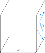
One way is to contemplate “large” extra dimensions of size [38]. Imagine there are extra dimensions in addition to our three-dimensional space. If you place two test masses at a distance much shorter than , the field lines of gravity spread out into dimensions and the force decreases as the surface area . However, if the distance is longer than , there is a limit to which how much the field lines can spread because they are squeezed within the size . Therefore, the force decreases only as for , reproducing the usual inverse square law of gravity. It turns out that the inverse square law is tested only down to 44 m [39] (even though this is very impressive!) and extra dimensions smaller than that are allowed experimentally.
Matching two expressions for the gravitational force at , we can related the Newton’s constant in dimensions to the Newton’s constant in three dimensions
| (3.4) |
and hence . In the natural unit , the mass scale of gravity is related to the Planck scale by . Even if the true energy scale of quantum gravity is at TeV, we may find an apparent scale of gravity to be GeV. Then the required size of extra dimensions is
| (3.5) |
Obviously the case is excluded because is even bigger than 1AU cm. The case is just excluded by the small-scale gravity experiment, while is completely allowed.
If we don’t see the extra dimensions directly, what do they do to us? Let us look at the case of just one extra dimension with periodic boundary condition . Then all particles have wave functions on the coordinate that satisfies . They can of course depend on the usual four-dimensional space time , too. One can expand it in Fourier modes
| (3.6) |
The momentum along the direction is , and the total energy of the particle is
| (3.7) |
Namely that you find a tower of particles of mass , called Kaluza–Klein states.
Of course, the standard model is tested down to cm, and we have not found Kaluza–Klein excitation of electron, etc. This is not a problem if we are stuck on a three-dimensional sheet (three-brane) embedded inside the dimensional space. The branes are important objects in string theory and it is easy to get particles with gauge interactions stuck on them. The brane may be freely floating inside extra dimensions or may be glued at singularities (e.g., orbifold fixed points). The simplest way to use large extra dimensions is to assume that only gravity is spread out in extra dimensions, while the standard model particles are all on a three-brane.
Cosmology with large extra dimension is an iffy subject, however. The Kaluza–Klein excitation of gravitons can be produced in early universe and the cosmology would be different from the standard Friedmann univese (see, e.g., [40]). I will not get into this discussion here.
Instead of models with large extra dimensions, models with small extra dimensions of size cm are also interesting,101010Historically, unified theories and string theory assumed cm. TeV-sized extra dimensions are much larger than this, but I’m calling them “small” for the sake of distinction from the large extra dimensions. which allow for normal cosmology below TeV temperatures. This would also allow us standard model particles to live in extra dimensions, too, because our Kaluza–Klein excitations have been too heavy to be produced at accelerators so far. There are many versions of small extra dimensions.
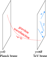
One very popular version is warped extra dimension [41]. Instead of flat metric in the extra dimensions, it sets up an exponential behavior. It is something like Planck scale varies from GeV to TeV as you go across the 5th dimension. Therefore, physics does end at TeV if you on one end of the 5th dimension, while it keeps going to GeV on the other end. The hierarchy problem may be solved if Higgs resides on (or close to) the “TeV brane.” This set up attracted a lot of attention because the bulk is actually a slice of anti-de Sitter space which has nice features of preserving supersymmetry, leading to AdS/CFT correspondence [42], etc. It is also possible to obtain quite naturally from string theory [43]. In a grand unified model from warped extra dimension, the proton longevity is an issue which is solved by a symmetry, and the lightest -charged particle (LZP) is a candidate for dark matter [44].
It is also possible to have the “flat” extra dimension at the TeV scale and put all the standard model particles in the 5D bulk, called Universal Extra Dimension (UED) [45]. It is tricky to get chiral fermions in four dimensions if they are embedded in higher dimensional space. If you start out with five-dimensional Dirac equation
| (3.8) |
the Fourier-mode expansion for the mode gives
| (3.9) |
After a chiral rotation , the second term turns into the usual mass term without . The problem is that here are always two eigenvalues and you find both left- and right-handed fermions with the same quantum numbers. Namely, you get Dirac fermion, not Weyl fermion. Then you don’t get the standard model that distinguishes left from right. In terms of spectrum, what is on the left of Fig. 8 is the spectrum because the Fourier modes and give the degenerate mass each of them with its own Dirac fermion.

The trick to get chiral fermions is to use an orbifold Fig. 9. Out of a circle (), you identify points and to get a half-circle . There are two special points, and , that are identified only with themselves called “fixed points.” In addition, we take the boundary condition that . For , we use for and for , without the degeneracy between and . For , only survives with the wave function . This way, we keep only a half of the states as shown in Fig. 8, and we can get chiral fermions. As a consequence, we find the system to have a symmetry under , under which modes with even are even and odd odd. This symmetry is called KK parity and the lightest KK state (LKP) becomes stable. At the tree-level, all first Kaluza–Klein states are degenerate .111111Here I’ve ignored possible complications due to brane operators and electroweak symmetry breaking. Radiative corrections split their masses, and typically the first Kaluza–Klein excitation of the boson is the LKP [46]. Because the mass splittings are from the loop diagrams, they are small. Similarly to supersymmetry, there is a large number of new particles beyond the standard model, namely Kaluza–Klein excitations. Its collider phenomenology very much resembles that of supersymmetry and it is not trivial to tell them apart at the LHC (dubbed “bosonic supersymmetry” [47]).

4 Evidence for Dark Matter
Now we turn our attention to the problem of non-baryonic dark matter in the universe. Even though this is a sudden change in the topic, you will see soon that it is connected to the discussions we had on physics beyond the standard model. We first review basics of observational evidence for non-baryonic dark matter, and then discuss how some of the interesting candidates are excluded. It leads to a paradigm that dark matter consists of unknown kind of elementary particles. By a simple dimensional analysis, we find that a weakly coupled particle at the TeV-scale naturally gives the correct abundance in the current universe. We will take a look at a simple example quite explicitly so that you can get a good feel on how it works. Then I will discuss more attractive dark matter candidates that arise from various models of physics beyond the standard model I discussed in the previous section.
The argument for the existence of “dark matter,” namely mass density that is not luminous and cannot be seen in telescopes, is actually very old. Zwicky back in 1933 already reported the “missing mass” in Coma cluster of galaxies. By studying the motion of galaxies in the cluster and using the virial theorem (assuming of course that the galactic motion is virialized) he determined the mass distribution in the cluster and reported that a substantial fraction of mass is not seen. Since then, the case for dark matter has gotten stronger and stronger and most of us regard its existence established by now. I refer to a nice review for details [48] written back in 1997, but I add some important updates since the review.
Arguably the most important one is the determination of cosmological parameters by the power spectrum of CMB anisotropy. In the fit to the power-law flat CDM model gives and [49]. The point here is that these two numbers are different. Naively subtracting the baryon component, and adding the errors by quadrature, I find at a very high precision. This data alone says most of the matter component in the universe is not atoms, something else.
Another important way to determine the baryon density of the universe is based on Big-Bang Nucleosynthesis (BBN). The baryon density is consistent with what is obtained from the CMB power spectrum, from five best measurements of deuterium abundance [50] using hydrogen gas at high redshift (and hence believed to be primordial) back-lit by quasars. This agrees very well with the CMB result, even though they refer to very different epochs: MeV for BBN while eV for CMB. This agreement gives us confidence that we know very well.
A novel technique to determine uses large-scale structure, namely the power spectrum in galaxy-galaxy correlation function. As a result of the acoustic oscillation in the baryon-photon fluid, the power spectrum also shows the “baryon oscillation” which was discovered only the last year [51]. Without relying on the CMB, they could determine . Again this is consistent with the CMB data, confirming the need for non-baryonic dark matter.
I’d like to also mention a classic strong evidence for dark matter in galaxies. It comes from the study of rotation curves in spiral galaxies. The stars and gas rotate around the center of the galaxy. For example, our solar system rotates in our Milky Way galaxy at the speed of about 220 km/sec. By using Kepler’s law, the total mass within the radius and the rotation speed at this radius are related by
| (4.1) |
Once the galaxy runs out of stars beyond a certain , the rotation speed is hence expected to decrease as . This expectation is not supported by observation.
You can study spiral galaxies which happen to be “edge-on.” At the outskirts of a galaxy, where you don’t find any stars, there is cold neutral hydrogen gas. It turns out you can measure the rotation speed of this cold gas. A hydrogen atom has hyperfine splitting due to the coupling of electron and proton spins, which corresponds to the famous cm line emission. Even though the gas is cold, it is embedded in the thermal bath of cosmic microwave background whose temperature 2.7 K is hot compared to the hyperfine excitation K.121212If we had lived in a universe a hundred times larger, we would have lost this opportunity of studying dark matter content of the galaxies! Therefore the hydrogen gas is populated in both hyperfine states and spontaneously emits photons of wavelength 21 cm by the M1 transition. This can be detected by radio telescopes. Because you are looking at the galaxy edge-on, the rotation is either away or towards us, causing Doppler shifts in the 21 cm line. By measuring the amount of Doppler shifts, you can determine the rotation speed. Surprisingly, it was found that the rotation speed stays constant well beyond the region where stars cease to exist.

I mentioned this classic evidence because it really shows galaxies are filled with dark matter. This is an important point as we look for signals of dark matter in our own galaxy. It is not easy to determine how much dark matter there is, however, because eventually the hydrogen gas runs out and we do not know how far the flat rotation curve extends. Nonetheless, it shows the galaxy to be made up of a nearly spherical “halo” of dark matter in which the disk is embedded.
5 What Dark Matter Is Not
We don’t know what dark matter is, but we have learned quite a bit recently what it is not. I have already discussed that it is not ordinary atoms (baryons). I mention a few others of the excluded possibilities.
5.1 MACHOs
The first candidate for dark matter that comes to mind is some kind of astronomical objects, namely stars or planets, which are is too dark to be seen. People talked about “Jupiters,” “brown dwarfs,” etc. In some sense, that would be the most conservative hypothesis.131313Somehow I can’t call primordial black holes a “conservative” candidate without chuckling. Because dark matter is not made of ordinary atoms, such astronomical objects cannot be ordinary stars either. But one can still contemplate the possibility that it is some kind of exotic objects, such as black holes. Generically, one refers to MACHOs which stand for MAssive Compact Halo Objects.
Black holes may be formed by some violent epochs in Big Bang (primordial black holes or PBHs) [53] (see also [54]). If the entire horizon collapses into a black hole, which is the biggest mass one can imagine consistent with causality, for example in the course of a strongly first order phase transition, the black hole mass would be
| (5.1) |
Therefore, there is no causal mechanism to produce PBHs much larger than assuming that universe has been a normal radiation dominated universe for MeV to be compatible with Big-Bang Nucleosynthesis. Curiously, one finds if it formed at the QCD phase transition MeV [55]. On the other hand, PBHs cannot be too small because otherwise they emit Hawking radiation of temperature that would be visible. The limit from diffuse gamma ray background implies .
How do we look for such invisible objects? Interestingly, it is not impossible using the gravitational microlensing effects [56]. The idea is simple. You keep monitoring millions of stars in nearby satellite galaxies such as Large Magellanic Cloud (LMC). Meanwhile MACHOs are zooming around in the halo of our galaxy at km/s. By pure chance, one of them may pass very close along the line of sight towards one of the stars you are monitoring. Then the gravity would focus light around the MACHO, effectively making the MACHO a lens. You typically don’t have a resolution to observe distortion of the image or multiple images, but the focusing of light makes the star appear temporarily brighter. This is called “microlensing.” By looking for such microlensing events, you can infer the amount of MACHOs in our galactic halo.
I’ve shown calculations on the deflection angle by the gravitational lensing and the amplification in the brightness in the appendix. (Just for fun, I’ve also added some discussions on the strong lensing effects.) The bottom line is that you may expect the microlensing event at the rate of
| (5.2) |
towards the LMC, with the duration of
| (5.3) |
where () is the distance between the MACHO and us (the lensed star).
Two collaborations, the MACHO collaboration and the EROS collaboration, have looked for microlensing events. The basic conclusion is that MACHOs of mass –30 cannot make up 100% of our galactic halo (Fig. 11). See also [58, 57].

Even though the possibility of MACHO dark matter may not be completely closed, it now appears quite unlikely. The main paradigm for the dark matter of the universe has shifted from MACHOs to WIMPs.
5.2 Neutrinos
Having discovered neutrinos have finite mass, it is also natural to consider neutrinos to be dark matter candidate. As a matter of fact, neutrinos are a component of dark matter, contributing
| (5.4) |
It is an attractive possibility if the particles which we already know to exist could serve as the required non-baryonic dark matter.
However, as Sergio Pastor discussed in his lectures, neutrinos are not good candidates for the bulk of dark matter for several reasons. First, there is an upper limit on neutrino mass from laboratory experiments (tritium beta decay) eV [59]. Combined with the smallness of mass-squared differences eV2 and eV2, electron-volt scale neutrinos should be nearly degenerate. Then the maximum contribution to the matter density is . This is not enough.
Second, even if the laboratory upper limit on the neutrino mass turned out to be not correct, there is a famous Tremaine-Gunn argument [60]. For the neutrinos to dominate the halo of dwarf galaxies, you need to pack them so much that you would violate Pauli exclusion principle. To avoid this, you need to make neutrinos quite massive eV so that you don’t need so many of them [61]. This obviously contradicts the requirement that .
Third, neutrinos are so light that they are still moving at speed of light (Hot Dark Matter) at the time when the structure started to form, and erase structure at small scales. Detailed study of large scale structure shows such a hot component of dark matter must be quite limited. The precise limit depends on the exact method of analyses. A relatively conservative limit says eV [62] while a more aggressive limit goes down to 0.17 eV [63]. Either way, neutrinos cannot saturate what is needed for non-baryonic dark matter.
In fact, what we want is Cold Dark Matter, which is already non-relativistic and slowly moving at the time of matter-radiation equality eV. Naively a light (sub-electronvolt) particle would not fit the bill.
A less conservative hypothesis may be to postulate that there is a new heavy neutrino (4th generation). This is a prototype for WIMPs that will be discussed later. It turns out, however, that the direct detection experiments and the abundance do not have a compatible mass range. Namely the neutrinos are too strongly coupled to be the dark matter!
5.3 CHAMPs and SIMPs
Even though people do not talk about it any more, it is worth recalling that dark matter is unlikely be charged (CHAMP) [64] or strongly interacting (SIMP) [65]. I simply refer to papers that limit such possibilities, from a multitude of search methods that include search for anomalously heavy “water” molecule in the sea water, high-energy neutrinos from the center of the Earth from annihilated SIMPs accumulated there, collapsing neutron stars that accumulate CHAMPs, etc.141414I once got interested in the possibility that Jupiter is radiating heat more than it receives from the Sun because SIMPs are annihilating at its core [66]. It does not seem to explain heat from other Jovian planets, however, once empirical limits on SIMPs are taken into account.
6 WIMP Dark Matter
WIMP, or Weakly Interactive Massive Particle, is the main current paradigm for explaining dark matter of the universe. With MACHOs pretty much gone, it is indeed attractive to make a complete shift from astronomical objects as heavy as GeV to “heavy” elementary particles of mass GeV. I will discuss why this mass scale is particularly interesting.
6.1 WIMP
The idea of WIMP is very simple. It is a relatively heavy elementary particle so that accelerator experiments so far did not have enough energy to create them, namely GeV. On the other hand, the Big Bang did once have enough energy to make them.
Let us follow the history from when . WIMPs were created as much as any other particles. Once the temperature dropped below , even the universe stopped creating them. If they are stable, whatever amount that was produced was there, and the only way to get rid of them was to get them annihilating each other into more mundane particles (e.g., quarks, leptons, gauge bosons). However, the universe expanded and there were fewer and fewer WIMPs in a given volume, and at some point WIMPs stopped finding each other. Then they could not annihilate any more and hence their numbers become fixed (“freeze-out”). This way, the universe could still be left with a certain abundance of WIMPs. This mechanism of getting dark matter is called “thermal relics.”
Let us make a simple estimate of the WIMP abundance. In radiation dominated universe, the expansion rate is given by
| (6.1) |
where GeV is the reduced Planck scale. For simple estimates, we regard and ignore many other factors of . Hence, . The entropy density is correspondingly
| (6.2) |
Given the thermally averaged annihilation cross section , and the number density of WIMPs , the annihilation rate of a WIMP is
| (6.3) |
The annihilation stops at the “freeze-out temperature” when , and hence
| (6.4) |
The yield of WIMPs is defined by . This is a convenient quantity because it is conserved by the expansion of the universe as long as the expansion is adiabatic, i.e., no new source of heat. This is due to the conservation of both the total entropy and total number of particles and their densities both scale as . The estimate of the yield is
| (6.5) |
Here, we defined . We will see later from more detailed calculations that . The abundance in the current universe is calculated using the yield and the current entropy density, divided by the current critical density,
| (6.6) |
We use and , where the current Hubble constant is with . In order of obtain , we need
| (6.7) |
Recall a typical annihilation cross section of a particle of mass by a relatively weak interaction of electromagnetic strength (e.g., ) is
| (6.8) |
To obtain the correct abundance, what we need is
| (6.9) |
This is a very interesting result. Namely, the correct abundance of thermal relics is obtained for a particle mass just beyond the past accelerator limits and where we expect new particles to exist because of the considerations of electroweak symmetry breaking and the hierarchy problem. In other words, it is exactly the right mass scale for a new particle!
In the next few sections, we will firm up this naive estimate by solving the Boltzmann equations numerically. We will also study a concrete model of a new particle for dark matter candidate and work out its annihilation cross section. In addition, we will see if we have a chance of “seeing” the dark matter particle in our galactic halo, or making it in future accelerator experiments. Then we will generalize the discussions to more theoretically attractive models of physics beyond the standard model.
6.2 Boltzmann Equation
You have already seen Boltzmann equation in lectures by Sabino Matarrese and I don’t repeat its derivations. We assume kinetic equilibrium, namely that each particle species has the Boltzmann distribution in the momentum space except for the overall normalization that is given by its number density. Considering the process of , where refers to a certain elementary particle, the Boltzmann equation for the number density for the particle is
| (6.10) |
Here, is the cross section common for the process and its inverse process assuming the time reversal invariance. The number densities with superscript 0 refer to those in the thermal equilibrium.
In the case of our interest, are “mundane” light (relativistic) particles in the thermal bath, and hence . In addition, we consider the annihilation , and hence . The Boltzmann equation simplifies drastically to
| (6.11) |
This time we pay careful attention to all numerical factors. We use
| (6.12) | |||||
| (6.13) | |||||
| (6.14) | |||||
| (6.15) |
Even though we start out at temperatures when are relativistic, eventually the temperature drops below and we can use non-relativistic approximations. Then the equilibrium number density can be worked out easily as
| (6.16) | |||||
Therefore
| (6.17) |
Changing the variables from to and to , the Boltzmann equation becomes
| (6.18) |
Here, we used and
| (6.19) |
It is useful to work out
| (6.20) |
Note that the annihilation cross section is insensitive to the temperature once the particle is non-relativistic .151515This statement assumes that the annihilation is in the -wave. If it is in the -wave, . Therefore the whole combination is just a dimensionless number. The only complication is that has a strong dependence on . We can further simplify the equation by introducing the quantity
| (6.21) |
We obtain
| (6.22) |
with
| (6.23) |
6.3 Analytic Approximation
Here is a simple analytic approximation to solve Eq. (6.22). We assume tracks for . On the other hand, we assume for because drops exponentially as . Of course this approximation has a discontinuity at , but the transition between these two extreme assumptions is so quick that it turns out to be a reasonable approximation. Then we can analytically solve the equation for and we find
| (6.24) |
Since , we obtain the simple estimate
| (6.25) |
Given this result, we can estimate as the point where drops down approximately to ,
| (6.26) |
and hence
| (6.27) | |||||
6.4 Numerical Integration
I’ve gone through numerical integration of the Boltzmann equation Eq. (6.22). Fig. 12 shows the -evolution of . You can see that it traces the equilibrium value very well early on, but after of about 20, it starts to deviate significantly and eventually asymptotes to a constant. This is exactly the behavior we expected in the analytic approximation studied in the previous section.
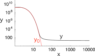
Fig. 13 shows the asymptotic values which we call . I understand this is a confusing notation, but we have to define the “freeze-out” in some way, and the analytic estimate in the previous section suggest that the asymptotic value is nothing but the freeze-out value . This is the result that enters the final estimate of the abundance and is hence the only number we need in the end anyway. It does not exactly agree with the estimate in the previous section, but does very well once I changed the offset in Eq. (6.27) from 24 to 20.43. Logarithmic dependence on is verified beautifully.

Putting everything back together,
| (6.28) |
As before, we use and , where the current Hubble constant is with . To obtain , we find GeV-2, confirming the simple estimate in Section 6.1.
6.5 The New Minimal Standard Model
Now we would like to apply our calculations to a specific model, called the New Minimal Standard Model [2]. This is the model that can account for the empirical facts listed in Section 2.1 with the minimal particle content if you do not pay any attention to the theoretical issues mentioned in Section 2.2. It accomplishes this by adding only four new particles to the standard model;161616The other three are the inflaton and two right-handed neutrinos. very minimal indeed! The dark matter in this model is a real scalar field with an odd parity , and its most general renormalizable Lagrangian that should be added to the Standard Model Eq. (LABEL:eq:LSM) is
| (6.29) |
The scalar field is the only field odd under , and hence the boson is stable. Because of the analysis in the previous sections, we know that if is at the electroweak scale, it may be a viable dark matter candidate as a thermal relic. This is a model with only three parameters, , , and , and actually the last one is not relevant to the study of dark matter phenomenology. Therefore this is a very predictive model where one can work it out very explicitly and easily.
SS1
{fmfgraph*}(100,40)
\fmflefti1,i2
\fmfrighto1,o2
\fmfdashesi1,v1,i2
\fmflabeli1
\fmflabeli2
\fmfvlabel=v1
\fmfdashes,label=v1,v2
\fmffermiono1,v2,o2
\fmflabelo1
\fmflabelo2
\fmfvlabel=v2
{fmffile}SS2
{fmfgraph*}(100,40)
\fmflefti1,i2
\fmfrighto1,o2
\fmfdashesi1,v1,i2
\fmflabeli1
\fmflabeli2
\fmfvlabel=v1
\fmfdashes,label=v1,v2
\fmfphotono1,v2,o2
\fmflabelo1
\fmflabelo2
\fmfvlabel=v2
{fmffile}SS3
{fmfgraph*}(100,40)
\fmflefti1,i2
\fmfrighto1,o2
\fmfdashesi1,v1,i2
\fmflabeli1
\fmflabeli2
\fmfvlabel=v1
\fmfdashes,label=v1,v2
\fmfdasheso1,v2,o2
\fmflabelo1
\fmflabelo2
\fmfvlabel=v2
{fmffile}SS4
{fmfgraph*}(100,40)
\fmflefti1,i2
\fmfrighto1,o2
\fmfdashesi1,v1
\fmfdashes,label=v1,v2
\fmfdashesv2,i2
\fmflabeli1
\fmflabeli2
\fmfvlabel=v1
\fmfvlabel=v2
\fmfdasheso1,v1
\fmfdasheso2,v2
\fmflabelo1
\fmflabelo2
{fmffile}SS5
{fmfgraph*}(100,40)
\fmflefti1,i2
\fmfrighto1,o2
\fmfdashesi1,v1,i2
\fmfdasheso1,v1,o2
\fmflabeli1
\fmflabeli2
\fmfvlabel=v1
\fmflabelo1
\fmflabelo2
To calculate the dark matter abundance, what we need to know is the annihilation cross section of the scalar boson . This was studied first in [68] and later in [69], but the third diagram was missing. In addition, there is a theoretical bounds on the size of couplings and so that they would stay perturbative up to high scales (e.g., Planck scale). The cosmic abundance is determined by and in addition to . Therefore on the plane, the correct cosmic abundance determines what should be. This is shown in Fig. 15. You can see that for a very wide range GeV–1.8 TeV, the correct cosmic abundance can be obtained within the theoretically allowed parameter space. For heavy , the cross section goes like and is independent of . This is why the contours are approximately straight vertically. For light , the cross section goes like . This is why the contours approximately have a fixed ratio. Note that when , the first two diagrams can hit the Higgs pole and the cross section can be very big even for small . This resonance effect is seen in Fig. 15 where GeV line reaches almost for GeV.
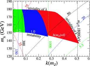
You may wonder why I am talking about as light as 5.5 GeV. Shouldn’t we have seen it already in accelerator experiments? Actually, no. The only interaction the boson has is with the Higgs boson which we are yet to see. Therefore, we could not have produced the boson unless we had produced the Higgs boson. That is why even such a light boson does not contradict data. In other words, it wouldn’t be easy to find this particle in accelerator experiments.
6.6 Direct Detection Experiments
How do we know if dark matter is indeed in the form of WIMP candidate you like? One thing we’d love to see is the direct detection of WIMPs. The idea is very simple. You place a very sensitive device in a quite location. WIMPs are supposed to be flying around in the halo of our galaxy with the typical speed of km/s . Because they are only very weakly interacting, they can go through walls, rocks, even the entire Earth with little trouble, just like neutrinos. For a mass of GeV, its typical kinetic energy is keV. If the WIMP (ever) scatters off an atomic nucleus, the energy deposit is only (at most) of this order of magnitude. It is a tiny energy deposit that is very difficult to pick out against background from natural radioactivity (typically MeV energies). Therefore you have to make the device very clean, and also place it deep underground to be shielded from the cosmic-ray induced backgrounds, most importantly neutrons ejected from the rocks by cosmic-ray muons. One you’ve done all this, what you do is to wait to see this little “kick” in your detector.
Let us do an order of magnitude estimate. The local halo density is estimated to be about GeV/cm3. The number density of WIMPs is . The flux of WIMPs is roughly . The elastic cross section of WIMP on neutron or proton may be spin-independent or spin-dependent. In the spin-independent case, the amplitude of the WIMP-nucleus cross section goes as (mass number) and hence the cross section on the nucleus goes as . Of course the detailed scaling is model-dependent, but in most phenomenological analyses (and also analyses of data) we assume . Let us also assume 56Ge as the detector material so that . Then the expected event rate is
| (6.30) |
To prepare a very sensitive device as big as 100 kg and make it very clean is a big job. You can see that your wait may be long.
Now back to the New Minimal Standard Model. The scattering of the boson off a proton comes from the -channel Higgs boson exchange. The coupling of the Higgs boson to the nucleon is estimated by the famous argument [70] using the conformal anomaly. The mass of the proton is proportional to the QCD scale ( are ignored and hence this is the three-flavor scale). It is related to the Higgs expectation value through the one-loop renormalization group equation as (we do not consider higher loop effects here)
| (6.31) |
where is some high scale and each quark mass is proportional to . The coupling of the Higgs to the proton is given by expanding the vacuum expectation value as , and hence
| (6.32) |
This allows us to compute the scattering cross section of the boson and the nucleon.
Sp {fmfgraph*}(100,40) \fmflefti1,i2 \fmfrighto1,o2 \fmffermioni1,v1,o1 \fmflabeli1 \fmfdashesi2,v2,o2 \fmfdashes,label=v1,v2 \fmflabeli2 \fmfvlabel=v2 \fmfvlabel=v1

The result is shown in Fig. 16 as the red solid line. The point is that the elastic scattering cross section tends to be very small. Note that a hypothetical neutrino of the similar mass would have a cross section of cm2 which is much much bigger than this. This is the typical WIMP scattering cross section. Superimposed is the limit from the CDMS-II experiment [71] and hence the direct detection experiments are just about to reach the required sensitivity. In other words, this simple model is completely viable, and may be tested by future experiments. For the resonance region , the coupling is very small to keep enough abundance and hence the direct detection is very difficult.
The future of this field is not only to detect WIMPs but also understand its identity. For this purpose, you want to combine the accelerator data and the direct detection experiments. The direct detection experiments can measure the energy deposit and hence the mass of the WIMP. It also measures the scattering cross section, even though it suffers from the astrophysical uncertainty in the estimate of the local halo density. On the other hand, assuming , the Higgs boson decays invisibly . Such an invisible decay of the light Higgs boson can be looked for at the LHC using the -fusion process. Quarks from both sides radiate an off-shell -boson that “fuse” in the middle to produce a Higgs boson. Because of the kick by the off-shell -boson, the quarks acquire in the final state and can be tagged as “forward jets.” Even though the Higgs boson would not be seen, you may “discover” it by the forward jets and missing [74]. The ILC can measure the mass of the Higgs precisely even when it decays dominantly invisibly (see, e.g., [75]) and possibly its width. Combining it with the mass from the direct detection experiments, you can infer the coupling and calculate its cosmic abundance. It would be a very interesting test if it agrees with the cosmological data . If it does, we can claim a victory; we finally understand what dark matter is!
6.7 Popular WIMPs
Superpartners of the photon and , and neutral Higgs bosons (there are two of them), mix among each other once symmetry breaks. Out of four such “neutralino” states, the lightest one is often the LSP171717Superpartner of neutrinos is not out of the question [80]. and is the most popular candidate for dark matter in the literature (see, e.g., [77, 78, 79] for some of the recent papers). One serious problem with the supersymmetric dark matter is that there are many parameters in the model. Even the Minimal Supersymmetric Standard Model (MSSM) has 105 more parameters than the standard model. It is believed that the fundamental theory determines all these parameters or at least reduces the number drastically, and one typically ends up with five or so parameters in the study. Depending on what parameter set you pick, the phenomenology may be drastically different. For the popular parameter set called CMSSM (Constrained MSSM, also called minimal supergravity or mSUGRA) with four parameters and one sign, see a recent study in [76]. I do not go into detailed discussions about any of them. I rather mention a few generic points.
First, we do get viable dark matter candidates from sub-TeV supersymmetry as desired by the hierarchy problem. This is an important point that shouldn’t be forgotten. Second, what exactly is the mass and composition of the neutralino depends on details of the parameter set. The supersymmetric standard model may not be minimal either; an extension with additional singlet called Next-to-Minimal Supersymmetric Standard Model (NMSSM) is also quite popular. Third, sub-TeV supersymmetry can be studied in great detail at LHC and (hopefully) ILC, so that we can measure their parameters very precisely (see [81] for the early work). One can hope to correlate the accelerator and underground data to fully test the nature of the dark matter [82]. Fourth, a large number of particles present in the model may lead to interesting effects we did not consider in the discussions above. I’ll discuss one of such effects briefly below.
Universal Extra Dimension (UED) is also a popular model. I’m sure Geraldine Servant will discuss dark matter in this model in her lectures because she is one of the pioneers in this area [86]. Because the LKP is stable, it is a dark matter candidate. Typically the first KK excitation of the gauge boson is the LKP, and its abundance can be reasonable. Its prospect for direct and indirect detection experiments is also interesting. See a review article that came out after Les Houches [87].
The most striking effect of having many particle species is the coannihilation [83]. An important example in the case of supersymmetry is bino and stau. Bino is the superpartner of the gaugino (mixture of photino and zino), and its annihilation cross section tends to be rather small partly because it dominantly goes through the -wave annihilation. If, however, the mass of the stau is not too far above bino, stau is present with the abundance suppressed only by ( assuming they are in chemical equilibrium . There are models that suggest the mass splitting is indeed small. The cross sections and etc tend to be much larger, the former going through the -wave and the latter with many final states. Therefore, despite the Boltzmann suppression, these additional contributions may win over . There are other cases where the mass splitting is expected to be small, such as higgsino-like neutralinos [84]. In the UED, the LKP is quite close in its mass to the low-lying KK states and again coannihilation is important.
6.8 Indirect Detection Experiments
On the experimental side, there are other possible ways of detecting signals of dark matter beyond the underground direct detection experiments and collider searches. They are indirect detection experiments, namely that they try to detect annihilation products of dark matter, not the dark matter itself. For annihilation to occur, you need some level of accumulation of dark matter. The possible sites are: galactic center, galactic halo, and center of the Sun. The annihilation products that can be searched for include gamma rays from the galactic center or halo, from the galactic halo, radio from the galactic center, anti-protons from the galactic halo, and neutrinos from the center of the Sun. Especially the neutrino signal complements the direct detection experiments because the sensitivity of the direct detection experiments goes down as because the number density goes down, while the sensitivity of the neutrino signal remain more or less flat for heavy WIMPs because the neutrino cross section rises as . You can look at a recent review article [85] on indirect searches.
7 Dark Horse Candidates
7.1 Gravitino
Assuming -parity conservation, superparticles decay all the way down to whatever is the lightest with odd -parity. We mentioned neutralino above, but another interesting possibility is that the LSP is the superpartner of the gravitino, namely gravitino. Since gravitino couples only gravitationally to other particles, its interaction is suppressed by . It practically removes the hope of direct detection. On the other hand, it is a possibility we have to take seriously. This is especially so in models with gauge-mediated supersymmetry breaking [88].
The abundance of light gravitinos is given by
| (7.1) |
if the gravitinos were thermalized. In most models, however, the gravitino is heavier and we cannot allow thermal abundance. The peculiar thing about a light gravitino is that the longitudinal (helicity ) components have a much stronger interaction if . Therefore the production cross section scales as , and the abundance scales as . Therefore we obtain an upper limit on the reheating temperature after the inflation [89, 90]. If the reheating temperature is right at the limit, gravitino may be dark matter.

There is however another mechanism of gravitino production. The abundance of the “LSP”is determined the usual way as a WIMP, while it eventually decays into the gravitino. This decay can upset the Big-Bang Nucleosynthesis [89], but it may actually be helpful for a region of parameter space to ease some tension among various light element abundances [91]. Note that the “LSP” (or more correctly NLSP: Next-Lightest Supersymmetric Particle) may be even electrically charged or strongly coupled as it is not dark matter. When superparticles are produced at colliders, they decay to the “LSP” inside the detector, which escapes and most likely decays into the gravitino outside the detector. If the “LSP” is charged, it would leave a charged track with anomalously high . It is in principle possible to collect the NLSP and watch them decay, and one may even be able to confirm the spin nature of the gravitino [92] and its gravitational coupling to matter [93].
If the gravitino is heavier than the LSP, its lifetime is calcuated as
| (7.2) |
It tends to decay after the BBN and upsets its success. Its production cross section scales as and hence . Depending on its mass and decay modes, one can again obtain upper limits on the reheating temperature. The case of hadronic decay for TeV is the most limiting case that requires GeV [94], causing trouble to many baryogenesis models.
7.2 Axion
One of the puzzles about the standard model I discussed earlier is why in QCD. A very attractive solution to this problem is to promote to a dynamical field, so that when it settles to the minimum of the potential, it automatically makes effectively zero [95]. The dynamical field is called axion, and couples (after integrating out some heavy fields) as
| (7.3) |
Here, is called axion decay constant which has a dimension of energy. The potential is given approximately as
| (7.4) |
and indeed the axion field settles to and the term vanishes. The axion mass is therefore
| (7.5) |
Various astrophysical limits basically require GeV and hence the axion is a very light boson (see, e.g., [96]). Most of these limits come from the fact that the axion can carry away energy from stars and would cool them too quickly, such as white dwarfs, red giants, and SN1987A. Models of such high are called “invisible axion” models because then the axion coupling is very weak to other particles, avoids these limits, and hence is very difficult to observe. There are two popular versions, KSVZ [97, 98] and DFSZ [99, 100] models.
In the early universe GeV, the axion potential looks so flat that it cannot tell where the minimum is.181818This is especially true for the axion because its mass originates from the QCD instaton effects which are suppressed by powers of the temperature in hot thermal bath [101]. Therefore we expect it starts out wherever it finds itself, mostly likely not at the minimum. The likely initial misplacement is of the order of . Now we would like to know what happens afterwards.
Let us consider a scalar field in an expanding universe. Neglecting the spatial variation and considering the time dependence alone, the equation of motion is
| (7.6) |
For a quadratic potential (mass term) , the equation is particularly simple and homogeneous,
| (7.7) |
It is useful to solve this equation for a constant (time-independent) first. For Fourier modes (of course we take the real part later on), we need to solve
| (7.8) |
and we find
| (7.11) | |||||
Therefore for (early universe), one of the solutions damps quickly , while the other is nearly stationary . This is because it is “stuck” by the friction term . On the other hand the field oscillates around the minimum as .
One can improve this analysis for time-dependent and in the radiation-dominated univese, by replacing by (adiabatic approximation). When (), we find
| (7.12) |
The second one is the solution that is stuck by the friction. On the other hand when ,
The field damps as , and its energy as , just like non-relativistic matter. In fact, a coherently oscillating homogeneous field can be regarded as a Bose–Einstein condensate of the boson at zero momentum state.
Therefore, the axion field can sit on the potential and does not roll down because of the large friction term when . On the other hand for later universe , it oscillates as a usual harmonic oscillator and dilutes as non-relativistic matter. This is why a very light scalar field can be a candidate for cold dark matter. Counterintuitive, but true. This way of producing cold dark matter is called “misalignment production” because it is due to the initial misalignment of the axion field relative to the potential minimum. Because the amount of misalignment is not known, we cannot predict the abundance of axion precisely. Assuming the misalignment of , GeV is the preferred range for axion dark matter.
There is a serious search going on for axion dark matter in the halo of our galaxy. In addition to the required coupling of the axion to gluons, most models predict its coupling to photons of the similar order of magnitude. The ADMX experiment places a high- cavity in a magnetic field. When an axion enters the cavity, this coupling would allow the axion to convert to a photon, which is captured resonantly by the cavity with a high sensitivity. By changing the resonant frequencies in steps, one can “scan” a range of axion mass. Their limit has just reached the KSVZ axion model [103, 104],191919They ignored theoretical uncertainty in the prediction of the axion-to-photon coupling, and the KSVZ model is not quite excluded yet [102]. and an upgrade to reach the DFSZ axion model using SQUID is in the works. See [105] for more on axion microwave cavity searches.
7.3 Other Candidates
I focused on the thermal reclic of WIMPs primarily because there is an attractive coincidence between the size of annihilation cross section we need for the correct abundance and the energy scale where we expect to see new partices from the points of view of electroweak symmetry breaking and hierarchy problem. Axion is not connected to any other known energy scale, yet it is well motivated from the strong CP problem. On the other hand, nature may not necessarily tell us a “motivation” for a particle she uses. Indeed, people have talked about many other possible candidates for dark matter. You may want to look up a couple of keywords: sterile neutrinos, axinos, warm dark matter, mixed dark matter, cold and fuzzy dark matter, -balls, WIMPZILLAs, etc. Overall, the candidates in this list range in their masses from eV to eV, not to mention still possible MACHOs eV. Clearly, we are making progress.
8 Cosmic Coincidence
Whenever I think about what the univese is made of, including baryons, photons, neutrinos, dark matter, and dark energy, what bothers me (and many other people) is this question: why do they have energy densities within only a few orders of magnitude? They could have been many orders of magnitude different, but they aren’t. This question is related to the famous “Why now?” problem. The problem is clear in Fig. 19. As we think about evolution of various energy densities over many decades of temperatures, why do we live at this special moment when the dark matter and dark energy components become almost exactly the same? I feel like I’m back to Ptolemy from Copernicus. We are special, not in space any more, but in time. Is that really so?

In Fig. 19, the radiation component goes down as , while the matter . The cosmological constant is by definition constant . Matter and meet now. When thinking about this problem, it is always tempting but dangerous to bring “us” into the discussion. Then we will be forced to talk about conditions for emergence of intelligent lifeforms, which we don’t know very well about. Instead, it may be better to focus on physical quantities; namely the triple coincidence problem that three lines with different slopes seem to more or less meet at a point. In fact, dimensional analysis based on TeV-scale WIMP suggests
| (8.1) |
which agrees with at the temperature K; this is about now! In order for the cosmological constant to meet at the same time, we suspect there is a deep reason
| (8.2) |
Indeed, is observationally about 2 meV, while meV. Maybe that is why we see a coincidence [106].
Actually, an exact coincidence does not leave a window for structure formation, which requires matter-dominated period. Fortunately, WIMP abundance is enhanced by weakness of the annihilation cross section, which goes like . This enhancement of matter relative to the triple coincidence gives us a window for matter domination and structure formation. May be that is why we seems to be in this triangle. But then, why is the baryon component also just a factor of five smaller than dark matter? Are they somehow related?
Oh well, we know so little.
9 Conclusions
In my lectures, I tried to emphasize that we are approaching an exciting time to cross new threshold of rich physics at the TeV energy scale in the next few years at the LHC. At the same time, the dark matter of the universe is now established to be not made of particles we know, requiring physics beyond the standard model. The main paradigm for dark matter now is WIMPs, TeV-scale particles produced by the Big Bang which naturally give the correct order of magnitude for its abundance. Even though nature may be tricking us by this coincidence, many of us (including I) think that there is indeed a new particle (or many of them) waiting to be discovered at the LHC (or ILC) that tells us something about the dark side of the universe. If this is so, I would feel lucky to be born to this age.
Appendix A Gravitational Lensing
Gravitational lensing is an important tool in many studies in cosmology and astrophysics. In this appendix I introduce the deflection of light in a spherically symmetric gravitational field (Schwarzschild metric)
Appendix A.1 Deflection Angle
Using the Schwarzschild metric ()
| (A. 1) |
where is the Schwarzschild radius. The Hamilton–Jacobi equation202020For an introduction to Hamilton–Jacobi equations, see http://hitoshi.berkeley.edu/221A/classical2.pdf. for light in this metric is
We separate the variables as
| (A. 3) |
where
Because the equation does not contain or explicitly, their functions must be constants,
| (A. 4) | |||||
| (A. 5) |
We can solve them immediately as
| (A. 6) | |||||
| (A. 7) |
Then Eq. (Appendix A.1) becomes
The dependence is only in the last two terms and hence
| (A. 8) |
is a constant which can be integrated explicitly if needed. Without a loss of generality, we can choose the coordinate system such that the orbit is on the - plane, and hence . In this case, and . Finally, the equation reduces to
| (A. 9) |
Therefore,
| (A. 10) |
Since , can be regarded as Legendre transform of the action, and hence the inverse Legendre transform gives
| (A. 11) |
Using the expression Eq. (A. 10), we find
| (A. 12) |
The closest approach is where the argument of the square root vanishes,
| (A. 13) |
It is useful to verify that the () limit makes sense. The closest approach is and hence , which is the impact parameter. The orbit Eq. (A. 12) is
| (A. 14) |
Change the variable to , and we find
| (A. 15) |
Hence , and
| (A. 16) |
Therefore which is nothing but a straight line.
To find the deflection angle, we only need to calculate the asymptotic angle . Going back to Eq. (A. 12), we need to calculate
| (A. 17) |
We would like to expand it up to the linear order in . If you naively expand the integrand in , the argument of the square root in the resulting expression can be negative for . To avoid this problem, we change the variable to :
| (A. 18) |
Using Eq. (A. 13), we write and obtain
| (A. 19) |
Expanding it to the linear order in , we find
| (A. 20) | |||||
The deflection angle is . It is easy to recover by looking at the dimensions, and we find .
It is also useful to know the closest approach to the first order in . We expand as . Then Eq. (A. 13) gives
| (A. 21) |
and hence
| (A. 22) |
Appendix A.2 Amplification in Microlensing
Once the deflection angle is known, it is easy to work out the amplification using simple geometric optics. Throughout the discussion, we keep only the first order in very small angles. Just by looking at the geometry in Fig. 20, the deflection angle is
| (A. 23) |
Here, is the impact parameter. When (exactly along the line of sight), the solution is simple:
| (A. 24) |
This is what is called the Einstein radius, in Paczynski’s notation [56]. For general , Eq. (A. 23) can be rewritten as
| (A. 25) |
which is Eq. (1) in the Packzynski’s paper. It has two solutions
| (A. 26) |
The solution with the positive sign is what is depicted in Fig. 20, while the solution with the negative sign makes the light ray go below the lens.

To figure out the amplification due to the gravitational lensing, we consider the finite aperture of the telescope (i.e., the size of the mirror). We assume an infinitesimal circular aperture. From the point of view of the star, the finite aperture is an image on the deflection plane of size , namely the plane perpendicular to the straight line from the star to the telescope where the lens is. The vertical aperture changes the impact parameter to a range (size of the mirror is ). Correspondingly, the image of the telescope is at .212121Note that this Taylor expansion is valid only when . For , we have to work it out more precisely; see next section. Using the solution Eq. (A. 26), we find that the vertical aperture always appears squashed (see Fig. 21),
On the other hand, the horizontal aperture is scaled as
| (A. 27) |
Because the amount of light that goes into the mirror is proportional to the elliptical aperture from the point of view of the star that emits light isotropically, the magnification is given by
The total magnificiation sums two images,
| (A. 28) |
with .222222The singular behavior for is due to the invalid Taylor expansion in . This is practically not a concern because it is highly unlikely that a MACHO passes through with . Note that the true image is actually not quite elliptic but distorted in this case. Basically, there is a significant amplification of the brightness of the star when the lens passes through the line of sight within the Einstein radius.
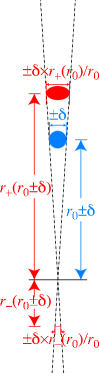
Appendix A.3 MACHO search
We estimate the frequency and duration of gravitational microlensing due to MACHOs in the galactic halo. The Large Magellanic Cloud is about 50kpc away from us, while we are about 8.5kpc away from the galactic center. The flat rotation curve for the Milky Way galaxy is about 220 km/sec (see Fig. 6 in [48]). The Einstein radius for a MACHO is calculated from Eq. (A. 24),
| (A. 29) |
To support the rotation speed of km/sec in the isothermal model of halo, we need the velocity dispersion . The average velocity transverse to the line of sight is
| (A. 30) |
The time it takes a MACHO to traverse the Einstein radius is
| (A. 31) |
about two months for and kpc. A microlensing event of duration shorter than a year can be in principle be seen.232323MACHO collaboration did even more patient scanning to look for microlensing events longer than a year [67].
The remaining question is the frequency of such microlensing events. It is the probability of a randomly moving MACHO coming within the Einstein radius of a star in the LMC. We will make a crude estimate. The flat rotation curves requires and hence the halo density . The number density of MACHOs, assuming they dominate the halo, is then . Instead of dealing with the Boltzmann (Gaussian) distribution in velocities, we simplify the problem by assuming that . From the transverse distance , only the fraction heads the right direction for the distance . Therefore the fraction of MACHOs that pass through the Einstein radius is
| (A. 32) |
We then integrate it over the depth with the number density. The distance from the solar system to the LMA is not the same as the distance from the galactic center because of the relative angle . The solar system is away from the galactic center by kpc. Along the line of sight to the LMA with depth , the distance from the galactic center is given by with . Therefore the halo density along the line of sight is
| (A. 33) |
The number of MACHOs passing through the line of sight towards a star in the LMA within the Einstein radius is
| (A. 34) | |||||
Pakzynski evaluates the optical depth, but I’d rather estimate a quantity that is directly relevant to the experiment, namely the rate of the microlensing events. Just by taking away,
| (A. 35) | |||||
The integral can be evaluated numerically. For kpc, kpc, , Mathematica gives 3.05. Then with , km/sec, we find
Therefore, if we can monitor about a million stars, we may see 5 microlensing events for a solar mass MACHO per year, even more for ligher ones.
Appendix A.4 Strong Lensing
Even though it is not a part of this lecture, it is fun to see what happens when . This can be studied easily with a slightly tilted coordinates in Fig. 22.

Using this coordinate system, we can draw a circle on the plane , and the corresponding image on the deflector plane is . The impact parameter is then which allows us to calculate using Eq. (A. 26) for each . Obviously is the same for the undistorted and distorted images. Fig. 23 shows a spectacular example with , , . Because , the Taylor expansion does not work, and the image is far from an ellipse.
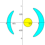
This kind of situation is not expected to occur for something as small as the mirror of a telescope, but may for something as big as a galaxy. When an image of a galaxy is distorted by a concentration of mass in the foreground, such as a cluster of galaxies, people have seen spectacular “strong lensing” effects, as shown in Fig. 24.

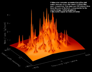
Acknowledgements
I’d like to express my gratitute to the organizers of the school, Francis Bernardeau and Christophe Grojean. I am especially indebted to Christophe for his patience waiting for this contribution. I also thank Adam Brown, Edoardo Di Napoli, Alexander Sellerholm, Ethan Siegel, Daniel Sunhede, Federico Urban, and Gilles Vertongen for our excursion to Tête Rousse. Matt Buckley kindly read and corrected the original manuscript. This work was supported in part by the U.S. Department of Energy under Contract DE-AC03-76SF00098, and in part by the National Science Foundation under grant PHY-04-57315.
References
- [1] G. Steigman, Int. J. Mod. Phys. E 15, 1 (2006) [arXiv:astro-ph/0511534].
- [2] H. Davoudiasl, R. Kitano, T. Li and H. Murayama, Phys. Lett. B 609, 117 (2005) [arXiv:hep-ph/0405097].
- [3] H. Murayama, Int. J. Mod. Phys. A 19, 1265 (2004) [arXiv:hep-ph/0312096].
- [4] C. A. Baker et al., Phys. Rev. Lett. 97, 131801 (2006) [arXiv:hep-ex/0602020].
- [5] M. Pospelov and A. Ritz, Annals Phys. 318, 119 (2005) [arXiv:hep-ph/0504231].
- [6] N. Arkani-Hamed and S. Dimopoulos, JHEP 0506, 073 (2005) [arXiv:hep-th/0405159].
- [7] V. Agrawal, S. M. Barr, J. F. Donoghue and D. Seckel, Phys. Rev. D 57, 5480 (1998) [arXiv:hep-ph/9707380].
- [8] R. Harnik, G. D. Kribs and G. Perez, Phys. Rev. D 74, 035006 (2006) [arXiv:hep-ph/0604027].
- [9] H. Murayama, Talk given at 22nd INS International Symposium on Physics with High Energy Colliders, Tokyo, Japan, 8-10 Mar 1994. Published in Proceedings, eds. S. Yamada and T. Ishii. World Scientific, 1995. 476p. [hep-ph/9410285].
- [10] V.F. Weisskopf, Phys. Rev. 56, 72 (1939).
-
[11]
M. Veltman,
Acta Phys. Polon. B12, 437 (1981);
S. Dimopoulos and S. Raby, Nucl. Phys. B192, 353 (1981);
E. Witten, Nucl. Phys. B188, 513 (1981);
M. Dine, W. Fischler and M. Srednicki, Nucl. Phys. B189, 575 (1981). -
[12]
R. Barbieri and G. F. Giudice,
Nucl. Phys. B306, 63 (1988);
G. W. Anderson and D. J. Castano, Phys. Lett. B347, 300 (1995) [hep-ph/9409419]; Phys. Rev. D 52, 1693 (1995) [hep-ph/9412322]. - [13] H. Murayama, “Supersymmetry phenomenology,” ICTP Summer School in Particle Physics, Trieste, Italy, 21 Jun - 9 Jul 1999. Published in PARTICLE PHYSICS 1999: Proceedings. Edited by G. Senjanovic and A.Yu. Smirnov. Singapore, World Scientific, 2000. 394p. (ICTP Series in Theoretical Physics, Vol. 16). arXiv:hep-ph/0002232.
- [14] S. P. Martin, arXiv:hep-ph/9709356.
- [15] L. E. Ibanez and G. G. Ross, Nucl. Phys. B 368, 3 (1992).
- [16] H. Murayama and D. B. Kaplan, Phys. Lett. B 336, 221 (1994) [arXiv:hep-ph/9406423].
- [17] C. D. Carone, L. J. Hall and H. Murayama, Phys. Rev. D 54, 2328 (1996) [arXiv:hep-ph/9602364].
- [18] E. Farhi and L. Susskind, Phys. Rept. 74, 277 (1981).
- [19] C. T. Hill and E. H. Simmons, Phys. Rept. 381, 235 (2003) [Erratum-ibid. 390, 553 (2004)] [arXiv:hep-ph/0203079].
- [20] C. Kolda and H. Murayama, JHEP0007, 035 (2000) [hep-ph/0003170].
- [21] C. Csaki, C. Grojean, H. Murayama, L. Pilo and J. Terning, Phys. Rev. D 69, 055006 (2004) [arXiv:hep-ph/0305237].
- [22] C. Csaki, C. Grojean, L. Pilo and J. Terning, Phys. Rev. Lett. 92, 101802 (2004) [arXiv:hep-ph/0308038].
- [23] H. Murayama, arXiv:hep-ph/0307293.
- [24] N. Arkani-Hamed, A. G. Cohen, E. Katz, A. E. Nelson, T. Gregoire and J. G. Wacker, JHEP 0208, 021 (2002) [arXiv:hep-ph/0206020].
- [25] N. Arkani-Hamed, A. G. Cohen, E. Katz and A. E. Nelson, JHEP 0207, 034 (2002) [arXiv:hep-ph/0206021].
- [26] D. B. Kaplan and H. Georgi, Phys. Lett. B 136, 183 (1984).
- [27] H. Georgi and D. B. Kaplan, Phys. Lett. B 145, 216 (1984).
- [28] N. S. Manton, Nucl. Phys. B 158, 141 (1979).
- [29] L. J. Hall, Y. Nomura and D. R. Smith, Nucl. Phys. B 639, 307 (2002) [arXiv:hep-ph/0107331].
- [30] G. von Gersdorff, N. Irges and M. Quiros, Nucl. Phys. B 635, 127 (2002) [arXiv:hep-th/0204223].
- [31] C. Csaki, C. Grojean and H. Murayama, Phys. Rev. D 67, 085012 (2003) [arXiv:hep-ph/0210133].
- [32] G. Burdman and Y. Nomura, Nucl. Phys. B 656, 3 (2003) [arXiv:hep-ph/0210257].
- [33] R. Contino, Y. Nomura and A. Pomarol, Nucl. Phys. B 671, 148 (2003) [arXiv:hep-ph/0306259].
- [34] K. Agashe, R. Contino and A. Pomarol, Nucl. Phys. B 719, 165 (2005) [arXiv:hep-ph/0412089].
- [35] H. C. Cheng, J. Thaler and L. T. Wang, JHEP 0609, 003 (2006) [arXiv:hep-ph/0607205].
- [36] H. C. Cheng and I. Low, JHEP 0408, 061 (2004) [arXiv:hep-ph/0405243].
- [37] S. Nussinov, Phys. Lett. B 165, 55 (1985).
-
[38]
N. Arkani-Hamed, S. Dimopoulos and G. Dvali,
Phys. Lett. B429, 263 (1998)
[hep-ph/9803315];
I. Antoniadis, N. Arkani-Hamed, S. Dimopoulos and G. Dvali, Phys. Lett. B436, 257 (1998) [hep-ph/9804398]. - [39] D. J. Kapner, T. S. Cook, E. G. Adelberger, J. H. Gundlach, B. R. Heckel, C. D. Hoyle and H. E. Swanson, Phys. Rev. Lett. 98, 021101 (2007) [arXiv:hep-ph/0611184].
- [40] L. J. Hall and D. R. Smith, Phys. Rev. D 60, 085008 (1999) [arXiv:hep-ph/9904267].
- [41] L. Randall and R. Sundrum, Phys. Rev. Lett. 83, 3370 (1999) [arXiv:hep-ph/9905221].
- [42] J. M. Maldacena, Adv. Theor. Math. Phys. 2, 231 (1998) [Int. J. Theor. Phys. 38, 1113 (1999)] [arXiv:hep-th/9711200].
- [43] S. B. Giddings, S. Kachru and J. Polchinski, Phys. Rev. D 66, 106006 (2002) [arXiv:hep-th/0105097].
- [44] K. Agashe and G. Servant, Phys. Rev. Lett. 93, 231805 (2004) [arXiv:hep-ph/0403143].
- [45] T. Appelquist, H. C. Cheng and B. A. Dobrescu, Phys. Rev. D 64, 035002 (2001) [arXiv:hep-ph/0012100].
- [46] H. C. Cheng, K. T. Matchev and M. Schmaltz, Phys. Rev. D 66, 036005 (2002) [arXiv:hep-ph/0204342].
- [47] H. C. Cheng, K. T. Matchev and M. Schmaltz, Phys. Rev. D 66, 056006 (2002) [arXiv:hep-ph/0205314].
- [48] G. G. Raffelt, “Dark matter: Motivation, candidates and searches,” 1997 European school of high energy physics, Proceedings edited by N. Ellis and M. Neubert. Geneva, Switzerland, CERN, 1998. 351p. (CERN-98-03) arXiv:hep-ph/9712538.
- [49] D. N. Spergel et al. [WMAP Collaboration], arXiv:astro-ph/0603449.
- [50] R. H. Cyburt, Phys. Rev. D 70, 023505 (2004) [arXiv:astro-ph/0401091].
- [51] D. J. Eisenstein et al. [SDSS Collaboration], Astrophys. J. 633, 560 (2005) [arXiv:astro-ph/0501171].
- [52] K. G. Begeman, A. H. Broeils and R. H. Sanders, Mon. Not. Roy. Astron. Soc. 249, 523 (1991).
- [53] B. J. Carr, Astrophys. J. 201, 1 (1975).
- [54] L. J. Hall and S. Hsu, Phys. Rev. Lett. 64, 2848 (1990).
- [55] K. Jedamzik, Phys. Rev. D 55, 5871 (1997) [arXiv:astro-ph/9605152].
- [56] B. Paczynski, Astrophys. J. 304, 1 (1986).
- [57] P. Tisserand et al. [EROS-2 Collaboration], arXiv:astro-ph/0607207.
- [58] C. Alcock et al. [MACHO Collaboration], arXiv:astro-ph/9803082.
- [59] W. M. Yao et al. [Particle Data Group], J. Phys. G 33, 1 (2006).
- [60] S. Tremaine and J. E. Gunn, Phys. Rev. Lett. 42, 407 (1979).
- [61] D. N. C. Lin and S. M. Faber, Astrophys. J. 266, L21 (1983).
- [62] S. Hannestad and G. G. Raffelt, JCAP 0611, 016 (2006) [arXiv:astro-ph/0607101].
- [63] U. Seljak, A. Slosar and P. McDonald, JCAP 0610, 014 (2006) [arXiv:astro-ph/0604335].
- [64] S. Dimopoulos, D. Eichler, R. Esmailzadeh and G. D. Starkman, Phys. Rev. D 41, 2388 (1990).
- [65] G. D. Starkman, A. Gould, R. Esmailzadeh and S. Dimopoulos, Phys. Rev. D 41, 3594 (1990).
- [66] M. Kawasaki, H. Murayama and T. Yanagida, Prog. Theor. Phys. 87, 685 (1992).
- [67] R. A. Allsman et al. [(Macho Collaboration) C Alcock], Astrop. J. Lett. 550, L169 (2001), arXiv:astro-ph/0011506.
- [68] J. McDonald, Phys. Rev. D 50, 3637 (1994), actually considered a complex .
- [69] C. P. Burgess, M. Pospelov and T. ter Veldhuis, Nucl. Phys. B 619, 709 (2001).
- [70] M. A. Shifman, A. I. Vainshtein and V. I. Zakharov, Phys. Lett. B 78, 443 (1978).
- [71] [CDMS Collaboration], arXiv:astro-ph/0405033.
- [72] R. Bernabei et al., Riv. Nuovo Cim. 26N1, 1 (2003).
- [73] R. Gaitskell and V. Mandic, http://dmtools.berkeley.edu/limitplots/
-
[74]
O. J. P. Eboli and D. Zeppenfeld,
Phys. Lett. B 495, 147 (2000)
[arXiv:hep-ph/0009158].
L. Neukermans and B. Di Girolamo, Observing an invisibly decaying Higgs boson in ATLAS via vector boson fusion, ATLAS note, ATL-PHYS-2003-006.
V. Buscher and K. Jakobs, Int. J. Mod. Phys. A 20, 2523 (2005) [arXiv:hep-ph/0504099]. - [75] G. Weiglein et al. [LHC/LC Study Group], Phys. Rept. 426, 47 (2006) [arXiv:hep-ph/0410364].
- [76] J. R. Ellis, K. A. Olive, Y. Santoso and V. C. Spanos, Phys. Lett. B 565, 176 (2003) [arXiv:hep-ph/0303043].
- [77] J. R. Ellis, K. A. Olive, Y. Santoso and V. C. Spanos, JHEP 0605, 063 (2006) [arXiv:hep-ph/0603136].
- [78] H. Baer, E. K. Park, X. Tata and T. T. Wang, JHEP 0608, 041 (2006) [arXiv:hep-ph/0604253].
- [79] R. Trotta, R. R. de Austri and L. Roszkowski, New Astron. Rev. 51, 316 (2007) [arXiv:astro-ph/0609126].
- [80] N. Arkani-Hamed, L. J. Hall, H. Murayama, D. R. Smith and N. Weiner, Phys. Rev. D 64, 115011 (2001) [arXiv:hep-ph/0006312].
- [81] T. Tsukamoto, K. Fujii, H. Murayama, M. Yamaguchi and Y. Okada, Phys. Rev. D 51, 3153 (1995).
- [82] E. A. Baltz, M. Battaglia, M. E. Peskin and T. Wizansky, Phys. Rev. D 74, 103521 (2006) [arXiv:hep-ph/0602187].
- [83] K. Griest and D. Seckel, Phys. Rev. D 43, 3191 (1991).
- [84] S. Mizuta and M. Yamaguchi, Phys. Lett. B 298, 120 (1993) [arXiv:hep-ph/9208251].
- [85] J. Carr, G. Lamanna and J. Lavalle, Rept. Prog. Phys. 69, 2475 (2006).
- [86] G. Servant and T. M. P. Tait, Nucl. Phys. B 650, 391 (2003) [arXiv:hep-ph/0206071].
- [87] D. Hooper and S. Profumo, arXiv:hep-ph/0701197.
- [88] M. Dine, A. E. Nelson and Y. Shirman, Phys. Rev. D 51, 1362 (1995) [arXiv:hep-ph/9408384]; M. Dine, A. E. Nelson, Y. Nir and Y. Shirman, Phys. Rev. D 53, 2658 (1996) [arXiv:hep-ph/9507378].
- [89] T. Moroi, H. Murayama and M. Yamaguchi, Phys. Lett. B 303, 289 (1993).
- [90] A. de Gouvea, T. Moroi and H. Murayama, Phys. Rev. D 56, 1281 (1997) [arXiv:hep-ph/9701244].
- [91] J. L. Feng, A. Rajaraman and F. Takayama, Phys. Rev. D 68, 063504 (2003) [arXiv:hep-ph/0306024].
- [92] W. Buchmuller, K. Hamaguchi, M. Ratz and T. Yanagida, Phys. Lett. B 588, 90 (2004) [arXiv:hep-ph/0402179].
- [93] J. L. Feng, A. Rajaraman and F. Takayama, Int. J. Mod. Phys. D 13, 2355 (2004) [arXiv:hep-th/0405248].
- [94] K. Kohri, T. Moroi and A. Yotsuyanagi, Phys. Rev. D 73, 123511 (2006) [arXiv:hep-ph/0507245].
- [95] R. D. Peccei and H. R. Quinn, Phys. Rev. Lett. 38, 1440 (1977).
- [96] H. Murayama, G. Raffelt, C. Hagmann, K. van Bibber and L. J. Rosenberg, “Axions and other very light bosons,” in [59].
- [97] J. E. Kim, Phys. Rev. Lett. 43, 103 (1979).
- [98] M. A. Shifman, A. I. Vainshtein and V. I. Zakharov, Nucl. Phys. B 166, 493 (1980).
- [99] A. R. Zhitnitsky, Sov. J. Nucl. Phys. 31, 260 (1980) [Yad. Fiz. 31, 497 (1980)].
- [100] M. Dine, W. Fischler and M. Srednicki, Phys. Lett. B 104, 199 (1981).
- [101] D. J. Gross, R. D. Pisarski and L. G. Yaffe, Rev. Mod. Phys. 53, 43 (1981).
- [102] M. Buckley and H. Murayama, in preparation.
- [103] S. J. Asztalos et al., Phys. Rev. D 69, 011101 (2004) [arXiv:astro-ph/0310042].
- [104] L. D. Duffy et al., Phys. Rev. D 74, 012006 (2006) [arXiv:astro-ph/0603108].
- [105] R. Bradley et al., Rev. Mod. Phys. 75, 777 (2003).
- [106] N. Arkani-Hamed, L. J. Hall, C. F. Kolda and H. Murayama, Phys. Rev. Lett. 85, 4434 (2000) [arXiv:astro-ph/0005111].
- [107] http://www.bell-labs.com/org/physicalsciences/projects/darkmatter/darkmatter1.html.