On the Hardness of Approximating Stopping and Trapping Sets

Abstract

We prove that approximating the size of stopping and trapping sets in Tanner graphs of linear block codes, and more restrictively, the class of low-density parity-check (LDPC) codes, is NP-hard. The ramifications of our findings are that methods used for estimating the height of the error-floor of moderate- and long-length LDPC codes based on stopping and trapping set enumeration cannot provide accurate worst-case performance predictions.

1 Introduction

In the past decade, the search for efficient and near-optimal decoding algorithms for linear block codes culminated with the rediscovery and generalization of the notion of sparse codes and iterative message passing algorithms. Although Maximum Likelihood (ML) decoding of linear block codes is NP-hard [5], iterative decoders can approach the Shannon limit of reliable communication with polynomial time complexity, provided that they operate on codes with long length that have sparse parity-check matrices, also known as LDPC codes [17]. Decoding is achieved via message passing on the Tanner graph of the code, a suitably chosen bipartite graphical representation of the code which contains a very small number of edges. On such graphs, probabilistic inference of the form of iterative message passing is known to have linear complexity in the code length.

The performance of linear block codes under iterative decoding, and the performance of LDPC codes in particular, depends on the structural properties of their chosen Tanner graphs. For each channel-decoder pair, there exist vertex configurations in the code graph on which the given iterative decoder fails. For some frequently encountered Discrete Memoryless Channels (DMCs), such configurations are known as near-codewords [26], trapping and stopping sets [12, 31], pseudocodewords [41, 22], and instantons [36].

It is known that ML decoders fail when transmission errors are confined to Tanner graph configurations containing codewords, while iterative decoders usually fail to make correct decisions on (strictly) larger sets of configurations. For example, iterative edge-removal (ER) decoders for signalling over the Binary Erasure Channel (BEC) fail on stopping sets [12], a subset of which are the codewords themselves. For the Additive White Gaussian Noise (AWGN) channel and sum-product decoding, failures arise due to subsets of vertices in the code graph that have similar structural properties as codewords, and are consequently termed near-codewords [26]. As a result, iterative decoders exhibit sub-optimal performance compared to ML decoders, and this performance loss most frequently manifests itself in terms of the emergence of error-floors in the Bit-Error-Rate (BER) curve of the code.

The error-floor phenomena is a problem of focal importance in the theory of iterative decoding, since many practical applications of codes on graphs require extremely low operational BERs. Since such low BERs are well beyond the scope of current Monte-Carlo simulation techniques, several methods were proposed for estimating the height of the error-floor through enumerating small stopping and small trapping sets [34], and exploring dominant instantons [31, 36]. These techniques operate fairly accurately for codes of very short and moderate length and small minimum pseudoweight, but they are time consuming, and no rigorous analytical study of the performance of these search procedures is known.

Recently, it was shown that the problem of finding the smallest stopping set in an arbitrary code graph is NP-hard to approximate up to a constant term [27]. In [40], it was shown that finding the smallest $k$-out set, which represents a straightforward generalization of the notion of a stopping set, is NP-hard as well. Despite the fact that $k$-out sets may lead to decoding failures similar to those caused by trapping sets, the results in [40] do not capture the fact that trapping sets are usually characterized in terms of two parameters. Furthermore, the notion of a trapping set is meaningful only in conjunction with a fixed decoding method. Finally, no hardness results for approximating $k$-out sets or more general trapping sets are currently known.

The main contributions of our work are three-fold. First, we improve upon the hardness results for approximating stopping sets, presented in [27]. Furthermore, we introduce the notion of a cover stopping set, and show that the problem of finding such a set of smallest cardinality in an arbitrary Tanner graph is NP-hard. Second, we provide a set of new results regarding the hardness of finding trapping sets for Gallager A decoder (GA) [4], the Zyablov-Pinsker (ZP) decoder [43, 42], and the product-sum decoder. The third, and most important finding presented in the paper is that these hardness results carry over to the case of LDPC code graphs (provided that the notion of “low-density” is properly defined). We discuss the impact of these findings on the accuracy of estimating the error-floor based on trapping set enumeration techniques. In addition, we give a brief overview of the theory of fixed parameter tractability (FPT), and show that the minimum cover stopping set problem is FPT.

The paper is organized as follows. Section 2 introduces the trapping set structures under investigation, as well as their corresponding decoding algorithms. Section 3 provides a brief overview of a class of NP-hard problems that are used in the reduction proofs of our main results. Section 4 contains theorems regarding the hardness of approximating classes of trapping sets, while Section 5 specializes these results for the class of sparse code graphs and short code lengths. In Section 6 we briefly comment on the accuracy of error-floor estimation procedures relying on exhaustive trapping set enumeration techniques. In Section 7, we describe the notion of fixed parameter tractability and its implications for stopping and trapping set size estimation. Concluding remarks are given in Section 8.

(a) Stopping Set.

(b) ZP Trapping Set.

Figure 1: Examples of Stopping and ZP-Trapping Sets.

(a) AWGN $(a,b)$-Trapping Set.

(b) AWGN Elementary $(a,b)$-Trapping Set.

Figure 2: Examples of AWGN Trapping Sets.

2 Definitions and Problem Formulation

A binary, linear $[n,k,d]$ code $\mathcal{C}$ is a $k$-dimensional vector subspace of an $n$-dimensional vector space $F_{2}^{n}$. The generator matrix $M$ of the code $\mathcal{C}$ is a $k\times n$ matrix of full row-rank, with rows that correspond to basis vectors of the subspace. The parity-check matrix $H$ of $\mathcal{C}$ is the generator matrix of the null-space of the code. The matrix $H$ defines a bipartite graph $G=(L\cup R,E)$, with columns of $H$ indexing the variable nodes in $L$, and the rows of $H$ indexing the check nodes in $R$. For $i\in L$ and $j\in R$, $(i,j)\in E$ if and only if $H_{i,j}=1$. The graph $G$ is called the Tanner graph of $\mathcal{C}$ with parity-check matrix $H$. If the parity-check matrix of a code contains only a “small” number of non-zero entries, i.e., it is sparse, then the corresponding code is called a Low-Density Parity-Check (LDPC) code. A precise definition of the notion “small” will be given in Section 5.

For the remaining definitions in this section we need to introduce the following notation and definitions. For $S\subset L$, the notation $\Gamma(S)$ is reserved for the set of neighbors of $S$ in $R$. $G_{S}$ denotes the induced subgraph for $S\subset L$ which is defined as the graph on nodes $S\cup\Gamma(S)$ with edges $\{(u,v):u\in S,v\in\Gamma(S)\}$. Equivalently, $G_{S}$ is the Tanner graph of the punctured parity-check matrix of the code, consisting of the columns indexed by $S$. For any graph $G^{\prime}$, $V(G^{\prime})$ denotes the set of nodes of $G^{\prime}$ and $E(G^{\prime})$

Iterative decoders are a class of inference algorithms that operate on Tanner graphs of codes. These decoders are known to compute the maximum likelihood estimates of variables only on Tanner graphs free of cycles. Nevertheless, when applied to LDPC codes that contain cycles, they can approach the Shannon limit on optimal performance with complexity linear in the length of the code.

The messages passed between vertices of the Tanner graphs during iterative decoding depend on the characteristics of the transmission channel, and there usually exist many different iterative decoding methods that can be used for the same channel. For various decoder architectures specialized for the BEC, BSC, and AWGN channel, the interested reader is referred to [32]. For clarity of the future exposition, we briefly describe three of these procedures: the edge-removal (ER) algorithm, the Zyablov-Pinsker (ZP) bit-flipping method [12, 43, 42], and the regular Gallager A algorithm [7]. The first algorithm operates on outputs of the BEC, while the second two are designed for the BSC. A detailed description of different decoding procedures for signalling over the AWGN channel can be found in [31].

The ER algorithm is used for codes transmitted over the BEC channel, where the input to the channel is a vector $c_{1}c_{2}\ldots c_{n}\in\mathcal{C}$, and the output is a vector $v_{1}v_{2}\ldots v_{n}$ over the symbol alphabet $\{{0,1,e\}}$. For a BEC channel with erasure probability $p$, one has $\Pr[v_{i}=c_{i}]=1-p$, and $\Pr[v_{i}=e]=p$. The ER algorithm assigns to each vertex $i$ in $L$ of the Tanner graph of $\mathcal{C}$ the symbol $v_{i}$. It then iteratively searches for vertices in $R$ adjacent only to one $e$ symbol in $L$. Due to the even-parity restriction, the corresponding $c_{i}$ value for such a symbol can be uniquely determined. The decoder terminates either when the correct codeword is recovered or if every every parity-check vertex connected to one $e$ symbol is connected to at least two such symbols. In the latter case, we say that the decoder failed on a stopping set.

Definition 1 (BEC Stopping Sets).

Given a bipartite graph $G=(L\cup R,E)$, we say that $S\subset L$ is a stopping-set if the degree of each vertex in $\Gamma(S)$ in the induced subgraph $G_{S}$ is at least two.

Of independent interest is the problem of determining the size of the smallest stopping set $S$ such that $\Gamma(S)=R$, i.e., the smallest set of vertices that covers each check node in $R$ at least twice. We refer to such a set as the cover stopping set. If symbols corresponding to a cover stopping set are erased, then the decoding process terminates before proceeding with the first iteration, and no erasure can be corrected.

Assume next that the Tanner graph of $\mathcal{C}$ is left-regular, with degree $\ell$. For a BSC channel with error probability $p$, the word $v_{1}v_{2}\ldots v_{n}\in\{{0,1\}}^{n}$ and $\Pr[v_{i}=c_{i}]=1-p$, and $\Pr[v_{i}=\bar{c}_{i}]=p$. In the first iteration of ZP-decoding, the decoder scans for received symbols $v_{i}$ that are connected to $\ell$ unsatisfied parity-check equations. If symbols with such a property are encountered, the decoder flips their values sequentially. The procedure is repeated for vertices with $\ell-1$, $\ell-2$, …, $\ell-\lfloor(\ell-1)/2\rfloor$ unsatisfied check-equations. The decoder terminates by either recovering the correct codeword or by encountering a word for which each symbol is included in less than $\ell-\lfloor(\ell-1)/2\rfloor$ unsatisfied check-equations. In the latter case, we say that the decoder failed on a ZP trapping set.

Definition 2 (BSC ZP-Trapping Sets).

Let $G=(L\cup R,E)$ be a left-regular bipartite graph with degree $\ell$. We say that $S\subset L$ is a ZP-trapping set if the induced subgraph $G_{S}$ is such that all vertices in $S$ are connected to less than $\ell-\lfloor(\ell-1)/2\rfloor$ odd degree vertices in $G_{S}$.

Figure 3: Example of Majority Trapping Set.

Another frequently used iterative decoding algorithm for signaling over the BSC that has a complete characterization of trapping sets is the Gallager A algorithm for regular codes with left vertex degree $\ell=3$. The decoding rule is straightforward: unless all incoming massages to a variable node are identical, the variable node transmits its received symbol. Otherwise, the node transmits the consensus vote. On the other hand, the check-nodes pass on their parity estimates to their neighboring variable nodes.

Definition 3 (BSC GA-Trapping Sets).

Let $G=(L\cup R,E)$ be a bipartite graph with left-degree three, such that all vertices in $R$ have degree $r>3$. Let $T\subset L$ and let $G_{T}$ be the subgraph of $G$ induced by $T$. Let $O=\{v\in\Gamma(T):\deg_{G_{T}}(v)\mbox{odd}\}$. We say $T$ is a GA-trapping set with parameter $a$ if $|O|=a$ and if $|\Gamma(u)\cap O|\leq 1$ for each $u\in T$ and no two checks in $O$ have a common neighbor in $L\setminus T$.

For the AWGN channel, and message-passing algorithms, no precise analytic characterization of failing configurations is known. Extensive computer simulations [31, 24] show that errors are usually confined to near codewords, also known as trapping sets or instantons. Roughly speaking, trapping sets resemble codewords in so far that they result in a very small number of unsatisfied check equations (for codewords, this number equals zero). We focus our attention on three such configurations, defined below.

Definition 4 (AWGN $(a,b)$-Trapping Sets).

Given a bipartite graph $G=(L\cup R,E)$, we say that $S\subset L$ is an $(a,b)$-trapping set if $|S|=a$ and the induced subgraph is such that $\Gamma(S)$ has exactly $b$ vertices of odd degree. Similarly, we say that $S\subset L$ is an elementary $(a,b)$-trapping set if $b$ vertices in $\Gamma(S)$ have degree one, and $|\Gamma(S)|-b$ vertices have degree two.

Definition 5 (AWGN Majority Trapping Set).

Given a bipartite graph $G=(L\cup R,E)$ we say $S\subset L$ is good if the induced subgraph $G_{S}$ is such that the majority of vertices of $G_{S}$ in $\Gamma(S)$ have even degree. $T$ is a majority trapping set if $T$ and $L\setminus T$ are both good.

Examples of Tanner graphs including stopping sets, ZP-trapping sets, as well as AWGN trapping sets are shown in Figures 1, 2, and 3, respectively. Circles denote variable nodes in $L$, while squares denote check nodes in $R$ of the Tanner graph $G(L\cup R,E)$.

Complexity Theory:

A problem belongs to the class NP if it can be solved in polynomial time by a non-deterministic Turing machine. Alternatively, the complexity category of decision problems for which answers can be checked for correctness using a certificate and an algorithm with polynomial running time in the size of the input is known as the NP class. A problem is NP-hard if the existence of a deterministic polynomial time algorithm for the problem would imply the existence of deterministic polynomial time algorithms for every problem in NP. This consequence is widely believed to be false, and hence determining that a problem is NP-hard is a very strong indicator that the problem in computational intractable, i.e., no deterministic, polynomial time algorithm exists for the problem.

For optimization problems, there exists a large body of work that considers approximate solutions rather than exact solutions [39]. When minimizing a function subject to constraints, we say an algorithm is an $\alpha$-approximation algorithm if it always returns a solution whose value is at most a factor $\alpha$ greater than the value for the optimal solution. For some NP-hard problems, it is possible to show that it is also NP-hard to $\alpha$-approximate the problem. For a more thorough treatment of these and other subjects in complexity theory, the interested reader is referred to [20].

Our Results:

We are concerned with the worst-case computational complexity of the following problems.

1. MinStop: Find a stopping set of minimum cardinality.

2. MinCStop: Find a cover stopping set of minimum cardinality .

3. MinTrap_ZP: Find a ZP-trapping set of minimum cardinality.

4. MinTrap_GA: Given $a$, find a GA-trapping set of minimum cardinality.

5. MinTrap_AWGN: Given $a$, find an $(a,b)$-trapping set with minimum parameter $b$.

6. MinTrap_AWGN-elem: Given $b$, find an $(a,b)$-elementary trapping set with minimum parameter $a$.

7. MinTrap_AWGN-maj: Find a majority trapping set of minimum cardinality.

We show that there are no polynomial time algorithms for any of the above problems under standard complexity assumptions. Furthermore, there are no polynomial time algorithms that even approximate the optimal solutions to a guaranteed precision. Many of these hardness results also apply when we restrict our attention to Tanner graphs that correspond to LDPC codes. Our proofs can all be cast as reductions from the NP-hard Minimum Set Cover, Minimum Distance [37, 38, 15], and Maximum Three-Dimensional Matching problems [5]. These, and some other relevant problems subsequently referred to, are briefly described in the following section.

3 A Class of NP-hard problems

For completeness, we provide known NP hardness and approximation results for a class of combinatorial optimization problems that will be used in the proofs of Sections 3, 4, and 5. Most of the results presented in this section are available at [21].

1. The Minimum Set Cover Problem, MinSetCov: Given a set of sets ${\mathcal{S}}=\{S_{1},\ldots,S_{a}\}$ of $[b]$, find ${\mathcal{S}}^{\prime}\subset{\mathcal{S}}$ of minimum cardinality such that $\cup_{S\in{\mathcal{S}}^{\prime}}S=[b]$. It is NP-hard to $c\log N$-approximate MinSetCov [30] for some $c$ where $N$ is the description length of the problem. Even in the case that $|S_{i}\cap S_{j}|\leq 1$, for $1\leq i<j\leq a$, it can be shown that there exists no polynomial time $c\log N$-approximation algorithm unless $NP\subset ZTIME(N^{O(\log\log N)})$ [23] where $ZTIME(t)$ denotes the class of problems that have a probabilistic algorithm with expected running time $t$ and with zero error probability.

2. The Minimum Hitting Set Problem, MinHitSet: Given a set of subsets ${\mathcal{S}}=\{S_{1},\ldots,S_{b}\}$ of $[a]$, find a set $S^{\prime}$ of smallest cardinality, such that $|S^{\prime}\cap S_{i}|\geq 1$, for all $i=1,2,\ldots,b$. The MinHitSet problem is equivalent to the MinSetCov problem [2] and as a consequence it is also NP-hard to $(c\log N)$-approximate MinHitSet [30] for some $c>0$. In the case when $|S_{i}|=2$ for all $i\in[b]$ the problem is often called the vertex cover problem MinVertCov. The vertex cover problem, even when we have $|\{i:j\in S_{i}\}|\leq 3$ is NP-hard to approximate up to some constant $\alpha>1$.

3. The Maximum Three-Dimensional Matching Problem, MaxThreeDimMatch: Given a set $T\subset X\times X\times X$, determine if a set $S\subset T$ of size $|X|$ exists such that no elements in $S$ agree in any coordinate. This decision problem is NP-hard even if no element of $X$ appears more than $3$ times in the same coordinate of sets from $T$ [20].

4. The Maximum Likelihood Decoding Problem, MaxLikeDecode: Given a code $\mathcal{C}$ specified by an $m\times n$ parity-check matrix $H$ (we may assume $H$ has linearly independent rows), a vector $s\in F_{2}^{m}$, and an integer $\omega>0$, determine if there is a vector $x\in F_{2}^{n}$ with weight bounded from above by $\omega$ and such that $H\,x^{T}=s$. The MaxLikeDecode problem is NP-hard to approximate within any constant factor [1].

5. The Minimum Weight Codeword Problem, MinCodeword: Given a code $\mathcal{C}$ specified by an $n\times k$ generator matrix $M$ of full row-rank, find the smallest weight of a non-zero codeword. The MinCodeword problem is not approximable within any constant factor unless $NP\subset RP$, where RP is the set of decision problems for which there exists a randomized algorithm that is always correct on no instances and correct with probability 1/2 on yes instances.

4 Hardness of Approximation Results

4.1 Hardness of Approximation for MinStop

We start by showing that MinStop is not approximable within $o(\log\,N)$, where $N$ denotes the description length of the problem, unless $P=NP$. This results improves upon the finding in [27], where the weaker claim that MinStop cannot be approximated within any positive constant was proved. This improvement is a consequence of the fact that our proof relies on reduction from the MinSetCov, rather than the MinVertCov problem [27].

Theorem 1.

There exists a constant $c>0$ such that it is NP-hard to $(c\log N)$-approximate MinStop.

Proof.

The proof is by a reduction from MinSetCov. Let $b=\left|\cup_{i\in[a]}S_{i}\right|$, and without loss of generality, assume that $S\subset[b]$, for each $S\in{\mathcal{S}}.$ Form a bipartite graph $G=(L\cup R,E)$ with $L=\{u_{1},...u_{a},x,y\}$, $R=\{v_{1},...v_{b},w_{1},...,w_{a},z\}$, and edges

$$E=\{(u_{i},v_{j}):j\in S_{i}\}\cup\{(u_{i},w_{i}):i\in[a]\}\cup\{(x,v):v\in R\}\cup\{(y,v):v\in\{w_{1},...,w_{a},z\}\}\enspace.$$

An illustration of this graphical structure is given in Figure 4.

We show that $G$ has stopping distance $2+t$ if and only if the minimum set cover is of size $t$. Since there is no polynomial algorithm returning an $c\log N$ approximation for MinSetCov unless $P=NP$ (for some sufficiently small $c>0$), this establishes the theorem.

Let $S$ be a stopping set. Consequently,

1. If $\left(x\in S\mbox{ or }y\in S\right)$, then $\left(x\in S\mbox{ and }y\in S\right)$ since otherwise $d_{G_{S}}(z)=1$.

2. If $x\in S$ then $u_{i}\in S$ for some $i$ since otherwise $d_{G_{S}}(v_{j})=1$ for some $j\in[b]$.

3. If $u_{i}\in S$ then $\left(x\in S\mbox{ or }y\in S\right)$ since otherwise $d_{G_{S}}(w_{i})=1$.

Therefore, if $S$ is non-empty $x,y,u_{i}\in S$ for some $i\in[a]$. But then $d_{G_{S}}(v_{j})\geq 2$ for $j\in S_{i}$. However this means that for all $j\in[b],\ d_{G_{S}\setminus\{x,y\}}(v_{j})\geq 1$. Therefore, $S$ being a stopping set implies that the included $u_{i}$ nodes correspond to a covering of $[b]$. The nodes corresponding to a covering of $[b]$, in addition to $x$ and $y$, form a stopping set, since every node on the right hand side ($R$) is in the neighborhood and has degree at least two. Hence the size of the minimum stopping set of $G$ is exactly 2 plus the size of the minimum set cover. ∎

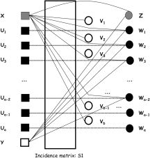
Figure 4: Reduction from MinSetCov to MinStop.

MinCStop:

The proof of Theorem 1 also implies that there exists a $c>0$ such that it is NP-hard to $(c\log n)$-approximate MinCStop. This is a consequence of the fact that the family of hard instances considered all had the property that the neighborhood of all stopping sets was all the check nodes. We next show that there exists a deterministic, polynomial-time, $O(\log n)$-approximation algorithm for MinCStop. This follows because we can relate MinCStop to MinHitSet as follows.

For each $r\in R$, create a set of sets $S_{r}$ that consists of all $(|\Gamma(r)|-1)$-subsets of $\Gamma(r)$. For example, if $\Gamma(r)=\{{a,b,c,d\}}$, then $S_{r}=\{{(a,b,c),(a,b,d),(a,c,d),(b,c,d)\}}.$ Let ${\mathcal{S}}=\{S_{r}:r\in R\}$. Then $Q\subset L$ is a hitting set for $\mathcal{S}$ iff it is a cover stopping set of $L$. This claim can be proved in a straightforward manner: if $\mathcal{S}$ contains at least one element, say $a$, from $\Gamma(r)$, then it must contain at least two elements from the same set since otherwise, the $(|\Gamma(r)|-1)$ set that does not contain $a$ will not be hit.

Consequently, any $\alpha$-approximation algorithm for MinHitSet can also be used to obtain an $\alpha$-approximation algorithm for MinCStop. For example the following simple greedy algorithm can be shown to be an $O(\log n)$-approximation algorithm for MinHitSet: At each step add the element that appears in the most sets from $\mathcal{S}$ can remove these sets from $\mathcal{S}$ can repeat until all the elements chosen appear in every set from $\mathcal{S}$.

The greedy algorithm searches for cover stopping sets by going through the list of variable nodes in decreasing order of their degree, and it is straightforward to see that the algorithm terminates after at most $(n-k)\,\delta_{\max}$ steps, where $\delta_{\max}$ denotes the largest degree of any check node in the Tanner graph of the code. As a consequence, this algorithm is especially well suited for LDPC codes, to be formally defined in Section 5.

Hardness under Stronger Assumptions:

Under the assumption that $NP\not\subset DTIME(N^{\operatorname{polylog}N})$, it was shown in [27] that there exists no polynomial time approximation algorithm for MinStop within $2^{(\log N)^{1-\epsilon}},$ for any $\epsilon>0$.

4.2 Hardness of Approximation for MinTrap_ZP, MinTrap_GA, and MinTrap_AWGN

We show next that the problems MinTrap_ZP, MinTrap_GA, and MinTrap_AWGN are computationally at least as hard as the MinCodeword problem.

Theorem 2.

For any constant $\alpha$, there is no polynomial-time $\alpha$-approximation algorithm for MinTrap_ZP, unless $RP=NP$.

Proof.

Recall that unless $RP=NP$, there is no polynomial time MinCodeword problem is $O(1)$-hard to approximate even under the restriction that the Tanner graph of the code is left regular. This follows directly from the results in [15].

Given a Tanner graph $G=(L\cup R,E)$ that is left regular say with degree $\lfloor(\ell-1)/2\rfloor+1$, for each node $u\in L$ create $\ell-\lfloor(\ell-1)/2\rfloor-1$ new nodes in $R$ each connected to $u$. Call the new Tanner graph $G^{\prime}$. Then any $S\subset L$ is a ZP-trapping set in $G^{\prime}$ iff $S$ is the support of a codeword in $G$. Hence any $\alpha$-approximation algorithm for MinTrap_ZP yields an $\alpha$-approximation algorithm for MinCodeword and the result follows. ∎

A very similar argument can be used to prove the following claim.

Theorem 3.

For any constant $\alpha$, there is no polynomial-time, $\alpha$-approximation algorithm for MinTrap_GA, unless $RP=NP$.

Proof.

Similarly as in the proof of Theorem 2, create for each node $u\in L$ one new node in $R$ each connected only to $u$. Call the new Tanner graph $G^{\prime}$. Then any $S\subset L$ is a GA-trapping set in $G^{\prime}$ iff $S$ is the support of a codeword in $G$. This follows due to the fact that the first condition in the definition of GA-trapping sets is identical to the ZP-restriction, with $\ell=3$. The second condition in the definition of an GA-trapping set is enforced automatically, since vertices in $L\setminus S$ cannot be connected to odd-degree check nodes in $G_{S}$ due to the fact that all such checks have degree one. Hence any $\alpha$-approximation algorithm for MinTrap_ZP yields an $\alpha$-approximation algorithm for MinCodeword and the result follows.

∎

Theorem 4.

For any constant $\alpha$, there is no polynomial-time, $\alpha$-approximation algorithm for MinTrap_AWGN, unless $RP=NP$.

Proof.

The proof is by a reduction from MinCodeword, and follows along similar lines as the proof of the above theorems. To this end, we construct the Tanner graph $(L\cup R,E)$ of the dual code $C^{\perp}$ where $L=\{u_{1},...u_{k}\},R=\{v_{1},...v_{n}\},$ and $E=\{(u_{i},v_{j}):M_{i,j}=1\}$ where $M$ denotes a generator matrix of the code of full row-rank. Note that for each $S\subset L$, $\Gamma(S)$ corresponds to a codeword. Hence, if we have an $\alpha$-approx to the min-trapping set problem for any $a$, then this gives an $\alpha$ approximation algorithm to the minimum weight codeword problem by running through all values of $a$ and taking the minimum of the resulting $b$’s. But, since it is impossible to $O(1)$-approximate MinCodeword in polynomial time unless $RP=NP$ [15], it is impossible to $O(1)$-approximate MinTrap_AWGN in polynomial time unless $RP=NP$. ∎

4.3 Hardness of Approximation for MinTrap_AWGN-elem

Theorem 5.

For any $\alpha$, it is NP-hard to $\alpha$-approximate MinTrap_AWGN-elem.

Proof.

The proof is based on showing that a polynomial time algorithm for solving MinTrap_AWGN-elem can be used for solving the MaxThreeDimMatch problem, and is based on similar arguments as those used for showing that MaxLikeDecode is NP-complete [5]. To this end, let us construct the matching incidence matrix $D$ as follows. Let the collection of ordered triples be $T\subset X\times X\times X$, where $|T|=t$, and $|X|=n$. Then $D$ is a $3\,n\times t$ dimensional zero-one matrix, with entries

$$1\leq i\leq n:\;\,D_{i,j}=1,\;\text{iff}\;\,x_{j}=i;$$

$$n+1\leq i\leq 2n:\;\,D_{i,j}=1,\;\text{iff}\;\,y_{j}=i;$$

$$2n+1\leq i\leq 3n:\;\,D_{i,j}=1,\;\text{iff}\;\,z_{j}=i.$$

As an example, the matrix $D$ for the set of triples

$$\{{(1,2,2),(3,2,1),(2,3,1),(1,2,3),(2,3,3),(3,1,3)\}}$$

over $X=\{{1,2,3\}}$ has the form

$$D=\left(\begin{array}[]{cccccc}1&0&0&1&0&0\\ 0&0&1&0&1&0\\ 0&1&0&0&0&1\\ 0&0&0&0&0&1\\ 1&1&0&1&0&0\\ 0&0&1&0&1&0\\ 0&1&1&0&0&0\\ 1&0&0&0&0&0\\ 0&0&0&1&1&1\\ \end{array}\right).$$

The set of triples $\{{(1,2,2),(2,3,1),(3,1,3)\}}$ is a maximum three-dimensional matching over the set $\{{1,2,3\}}$. Observe that all rows in the sub-matrix of $D$ induced by the three columns corresponding to these triples have Hamming weight one. This is a consequence of the defining constraint of the MaxThreeDimMatch problem that asserts that every element in $X$ appears at a given position of the matching exactly once.

Assume next that there exists a polynomial-time, $\alpha$-approximation algorithm for the MinTrap_AWGN-elem problem. Construct $D$ for a given matching problem, set $b=3\times n$, and run the MinTrap_AWGN-elem algorithm on $D$. If the algorithm the algorithm finds an elementary trapping set then it must have size $n$. Consider the corresponding set of $n$ columns indexed by a set of $n$ triples from $T$. Each row in the sub-matrix induced by the triples has weight one, which follows from the definition of an elementary trapping set. Consequently, these triples represent a matching for $T$. This implies that no polynomial time algorithm for the MinTrap_AWGN-elem problem exists, unless P=NP. ∎

4.4 Hardness of Approximation for MinTrap_AWGN-maj

First we prove a hardness of approximation result for the problem of finding the good set of minimum cardinality. Recall that a set $S\subset L$ us good if the majority of nodes in $\Gamma(S)$ have even degree in $G_{S}$. We call this problem MinGood. We will then use this to show a hardness of approximation result for MinTrap_AWGN-maj.

Our proof uses a reduction from MinCodeword. Let $H$ be the $n\times(n-k)$ parity check of some code. We may assume that the code specified by $H$ includes at least one codeword in addition to the zero vector. This gives rise to the graph $G^{\prime}=(L^{\prime}\cup R^{\prime},E^{\prime})$ where $L^{\prime}=\{x_{1},\ldots,x_{n}\},R^{\prime}=\{y_{1},\ldots,y_{m}\},$ and $E^{\prime}=\{(x_{i},y_{j}):H_{i,j}=1\}.$ We will create a bipartite graph $G=(L\cup R,E)$ by augmenting $G^{\prime}$ with graphical objects termed “ZigZag”s and “OrGate”s. These graphical objects will ensure that the minimum cardinality of a good set is approximately proportional to the minimum weight of any codeword.

4.4.1 The ZigZag

For each $x\in L^{\prime}$ we add a $\textup{{ZigZag}}(x)$ structure. This structure consists of $3(m-1)$ nodes, given by $L(\textup{{ZigZag}}(x))=\{v_{1},\ldots,v_{m-1}\},R(\textup{{ZigZag}}(x))=\{u_{1},\ldots,u_{m-1},w_{1},\ldots,w_{m-1}\},$ and edges,

$$E(\textup{{ZigZag}}(x))=\{(u_{i},v_{i}),(v_{i},w_{i}):i\in[m-1]\}\cup\{(v_{i},w_{i+1}:i\in[m-2]\}\cup\{(x,w_{1})\}\$$

The intuition behind the $\textup{{ZigZag}}(x)$ structure is that if $x$ is in the trapping set then the nodes $L(\textup{{ZigZag}}(x))$ will also be in the trapping set. For a subgraph $G^{\prime\prime}$ of $G$, and $S\in L$ we define

$$\operatorname{Disc}_{S}(G^{\prime\prime}) = |\{v\in\Gamma(S)\cap V(G^{\prime\prime}):d_{G_{S}}(v)\mbox{ even}\}|-|\{v\in\Gamma(S)\cap V(G^{\prime\prime}):d_{G_{S}}(v)\mbox{ odd}\}|.$$

Lemma 1.

For all $x\in S$, $\operatorname{Disc}_{S}(\textup{{ZigZag}}(x))\leq 0$ and $\operatorname{Disc}_{S}(\textup{{ZigZag}}(x))=0$ iff $\textup{{ZigZag}}(x)\cap L\subset S$.

Proof.

Note that

$$|\{v\in\Gamma(S)\cap V(\textup{{ZigZag}}(x)):d_{G_{S}}(v)\mbox{ odd}\}|\geq|\{v\in S\cap V(\textup{{ZigZag}}(x))|$$

with equality iff $L^{\prime}\cap V(\textup{{ZigZag}}(x))\subset S$ because each $v_{i}\in S$ is connected to $w_{i}$ which has degree 1. But for any $S$,

$$|\{v\in\Gamma(S)\cap V(\textup{{ZigZag}}(x)):d_{G_{S}}(v)\mbox{ even}\}|\leq|\{v\in S\cap V(\textup{{ZigZag}}(x))|\$$

with equality iff $L^{\prime}\cap V(\textup{{ZigZag}}(x))\subset S$. ∎

4.4.2 The OrGate

For each $y\in R^{\prime}$ we add $\textup{{OrGate}}(y)$, and let $\Gamma(y)\cap L^{\prime}=\{u_{1},\ldots,u_{k^{\prime}}\}$. Let $k=2^{\lceil\log_{2}k^{\prime}\rceil}$. The construction $\textup{{OrGate}}(y)$ consists two node sets $L(\textup{{OrGate}}(y))$ and $R(\textup{{OrGate}}(y))$. Consider a binary tree on the nodes $\{u_{1},\ldots,u_{k}\}$ where $u_{k^{\prime}+i}=u_{k^{\prime}}$ for $i\in[k-k^{\prime}]$. Then $L(\textup{{OrGate}}(y))$ consists of nodes corresponding to the internal nodes of the tree, i.e.

$$L(\textup{{OrGate}}(y))=\{v_{u_{1}\vee u_{2}},\ldots,v_{u_{k-1}\vee u_{k}},v_{u_{1}\vee u_{2}\vee u_{3}\vee u_{4}},\ldots,v_{u_{k-3}\vee u_{k-2}\vee u_{k-1}\vee u_{k}},\ldots,v_{u_{1}\vee u_{2}\vee\ldots\vee u_{k}}\}$$

For each internal node $v$ with children $u$ and $w$, we add four new check nodes $C(v):=\{c_{1}(v),c_{2}(v),c_{3}(v),c_{4}(v)\}$: all are connected $v$, the first and third are connected to $u$ and the first and second are connected to $w$. If $v$ is the root of the tree, we also add one more new check node which is connected only to $v$. We call this node $z$. Let $R(\textup{{OrGate}}(y))$ be the set of such nodes, and let $E(\textup{{OrGate}}(y))$ be the set of such edges. Finally, let

$$f(S,y)=\{v_{u_{i}\vee\ldots\vee u_{j}}\in L(\textup{{OrGate}}(y)):|S\cap\{u_{i},\ldots,u_{j}\}|\geq 1\}\enspace.$$

(a) $\textup{{OrGate}}(y)$

(b) $\textup{{ZigZag}}(x)$

(c) Ballast

Figure 5: Reduction from MinCodeword to MinTrap_AWGN-maj.

Lemma 2.

For all $y\in G_{S}\cap R$, $\operatorname{Disc}_{S}(\textup{{OrGate}}(y))\leq-1$ with equality if $S\cap L(\textup{{OrGate}}(y))=f(S,y)$.

Proof.

Consider the four check nodes $C(v)$ for some internal node $v$ of the tree used in the construction of $\textup{{OrGate}}(y)$. Let $u,w$ be the children of $v$ in the original binary tree tree. Then, if either $u,v,w\in S$ then $\operatorname{Disc}_{S}(C(v))\leq 0$ with equality iff $v\in S$ and at least one of $u,w\in S$. Consequently, if $\Gamma(y)\cap L^{\prime}\cap S\neq\emptyset$, $\operatorname{Disc}_{S}(\cup_{v}C(v))\leq 0$ with equality iff $S\cap L(\textup{{OrGate}}(y))=f(S,y)$. In particular, the root of the binary tree is in $S$ and therefore the final check node $z$ has odd degree. Therefore, if $\Gamma(y)\cap L^{\prime}\cap S\neq\emptyset$, $\operatorname{Disc}_{S}(\cup_{v}C(v))\leq-1$ with equality if $S\cap L(\textup{{OrGate}}(y))=f(S,y)$. ∎

4.4.3 Hardness of MinGood

Note that the graph $G$ that has been constructed has $|L|\leq mn+2n(n-k)$ and $|R|\leq(n-m)+n^{2}$.

Lemma 3.

$\operatorname{Disc}_{S}(G)\geq 0$ iff $S\cap L^{\prime}$ is a codeword and for each $x\in S\cap L^{\prime}$, $\textup{{ZigZag}}(x)\cap L\subset S$.

Proof.

According to Lemma 1 and 2,

$$\operatorname{Disc}_{S}(G) = \operatorname{Disc}_{S}(G^{\prime})+\sum_{x\in L^{\prime}}\operatorname{Disc}_{S}(\textup{{ZigZag}}(x))+\sum_{y\in R^{\prime}}\operatorname{Disc}_{S}(\textup{{OrGate}}(y))$$

$$\leq \operatorname{Disc}_{S}(G^{\prime})-\sum_{x\in L^{\prime}}I_{\textup{{ZigZag}}(x)\cap L\not\subset S}-|\Gamma(S)\cap R^{\prime}|.$$

Note that $\operatorname{Disc}_{S}(G^{\prime})\leq|\Gamma(S)\cap R^{\prime}|$ and therefore $\operatorname{Disc}_{S}(G)\geq 0$ implies that $d_{G_{S}}(y)$ is even for all $y\in R^{\prime}$ and $\textup{{ZigZag}}(x)\subset G_{S}$ for all $x\in S\cap L^{\prime}$. Again, according to Lemma 1 and 2 if $\forall y\in R^{\prime},\ d_{G_{S}}(y)=0\bmod 2$, and $\forall x\in S\cap L^{\prime},\ \textup{{ZigZag}}(x)\subset G_{S}$, then $\operatorname{Disc}_{S}(G)\geq 0$. ∎

Theorem 6.

For any constant $\alpha$, there is no polynomial-time, $\alpha$-approximation algorithm for MinGood, unless $RP=NP$.

Proof.

Assume that $S$ is a good set such that $S\leq\alpha\textsc{MinGood}$ for some constant $\alpha$. By Lemma 3 and Lemma 2,

$$|S|=|S\cap L^{\prime}|m+\sum_{y\in\Gamma(S\cap L^{\prime})}|f(S,y)|,$$

and $S\cap L^{\prime}$ corresponds to a codeword. But $\sum_{y\in\Gamma(S\cap L^{\prime})}|f(S,y)|\leq 2n(n-k)$, and so by setting $m$ sufficiently large we get a constant approximation for MinCodeword. But no such approximation exists unless $RP=NP$ [15]. ∎

4.4.4 Hardness of MinTrap_AWGN-maj

To achieve the hardness result for MinTrap_AWGN-maj we need to further augment our graph $G$ with multiple “Ballast” constructions. We call the resulting graph $G^{+}$. The intuition behind Ballast is that no nodes from Ballast will be chosen in $S$ while the multiple copies of Ballast will ensure that the complement of $S$ is also good. A single Ballast consists of nodes $L(\textup{{Ballast}})=\{u_{1},\ldots,u_{l}\}$, $R(\textup{{Ballast}})=\{v_{1},\ldots,v_{l},w_{2},\ldots,w_{l}\},$ and edges,

$$E(\textup{{Ballast}})=\{(u_{i},v_{i}):i\in[l]\}\cup\{(v_{i},u_{i+1}):i\in[l-1]\}\cup\{(v_{l},u_{1})\}\cup\{(u_{i},w_{i}):1\leq i\leq l-1\}\ .$$

We consider setting $l=n|L|$ and adding $|R|$ copies of Ballast to $G$.

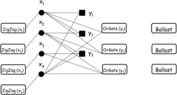
Figure 6: Combining the $\textup{{ZigZag}},\textup{{OrGate}},$ and Ballast constructions.

Lemma 4.

$\operatorname{Disc}_{S}(\textup{{Ballast}})\leq 1$ with equality iff $L(\textup{{Ballast}})\subset S$.

Proof.

Let $A=S\cap\{u_{1},\ldots,u_{l}\}$. Note that $\Gamma(A)$ contains at least $|A|-1$ nodes with odd degree with equality iff $L(\textup{{Ballast}})\subset S$. $\Gamma(A)$ contains at most $|A|$ nodes of even degree with equality iff $L(\textup{{Ballast}})\subset S$. ∎

Lemma 5.

Assuming there exists a non-zero codeword, there is a good set in $G$. Furthermore, any good set in $G$ is a trapping set for $G^{+}$.

Proof.

Let $S^{\prime}$ be the subset of $L^{\prime}$ corresponding to the minimum weight codeword. Let

$$S=S^{\prime}\cup\left(\bigcup_{x\in S^{\prime}}L(\textup{{ZigZag}}(x))\right)\cup\left(\bigcup_{y\in\Gamma(S^{\prime})}f(S,y)\right)\enspace.$$

Then $S$ is a good set in $G$. For the second part of the lemma note that by Lemma 4, for $S\subset L$, $\operatorname{Disc}_{\bar{S}}(G^{+})\geq|R|-|R|=0$. ∎

Theorem 7.

For any constant $\alpha$, there is no polynomial-time, $\alpha$-approximation algorithm for MinGood, unless $RP=NP$.

Proof.

Assume that $S$ is a trapping set such that $S\leq\alpha\textsc{MinTrap${}_{\mathrm{AWGN-maj}}$}$ for some constant $\alpha$. By Lemma 5, we know that $|S|\leq\alpha|L|$ and hence $S$ does not include all left hand side nodes of any copy of Ballast because doing so would imply that $|S|\geq|L(\textup{{Ballast}})|=n|L|$. But then by Lemma 4, we may assume that no nodes from Ballast are included in $S$ because removing all such nodes from $S$ increases $\operatorname{Disc}_{S}(G)$. Consequently $S$ must be a subset of $L$. Since any good subset of $L$ is a trapping set, $\textsc{MinGood}(G)=\textsc{MinTrap${}_{\mathrm{AWGN-maj}}$}(G^{+})$. But, by Theorem 6, there is no constant approximation of MinGood. ∎

5 Hardness of Approximation Results for Sparse Codes

The fact that a problem is NP-hard usually does not imply that a special instance of the problems is NP-hard. Since iterative decoding algorithms have both linear-time complexity and offer good decoding performance only for special classes of codes, it is important to establish the analogues of the results in Section 4 for such codes. We provide next a set of results establishing the hardness of approximating stopping and trapping sets for low-density parity-check (LDPC) codes.

LDPC codes are linear block codes for which the parity-check matrix $H$ is sparse -i.e., for which $H$ has a “small” number of non-zero entries. More formally, we define an LDPC code as follows. An LDPC code is a code with the property that each variable and check node in its Tanner graph $G=(L\cup R,E)$ has degree at most $\delta_{v}$ and $\delta_{c}$, respectively, for some constants $\delta_{v},\delta_{c}>2$ independent on $n$.

Theorem 8.

There exists a constant $\alpha>1$ such that it is NP-hard to $\alpha$-approximate MinStop in the Tanner graph of an LDPC code.

The proof follows along the same lines as the proof of NP-hardness using reduction from the problem MinVertCov problem [27]: Let $G=(V,E)$ be an undirected graph, which, without loss of generality, can be assumed to be connected and of vertex degree bounded from above by three. Furthermore, also assume that $|V|=n$, $|E|=m$, and that $E=\{{e_{1},\ldots,e_{m}\}}$, $V=\{{v_{1},\ldots,v_{n}\}}$. Without loss of generality, one can set $e_{1}=(v_{1},v_{2})\in E$. A bipartite graph $G_{vc}$ is constructed as follows: the left hand side vertices of the graph consist of nodes $L=L_{0}\cup L_{1}$, where $L_{0}=V$, and $L_{1}=\{{e^{\prime}_{1},\ldots,e^{\prime}_{m}\}}$. The right hand side vertices of the graph consist of nodes $R=R_{0}\cup R_{1}$, with $R_{0}=E$, and $R_{1}=\{{z_{1},\ldots,z_{m}\}}$. The set of edges of $G_{vc}$ is a collection of ordered pairs the following form:

$$~{}\{(e_{i}\in R_{0},u\in L_{0}),(e_{i}\in R_{0},v\in L_{0}):e_{i}=(u,v)\in E\}\cup\{(e_{i}\in R_{0},e^{\prime}_{i}\in L_{2}):1\leq i\leq m\}\cup$$

$$~{}\{(z_{i}\in R_{1},e^{\prime}_{i}\in L_{1}),(z_{i}\in R_{1},e^{\prime}_{i+1}\in L_{1}):1\leq i\leq m-1\}\cup\{(z_{m}\in R_{1},v_{1}\in L_{0}),(z_{m}\in R_{1},e^{\prime}_{1}\in L_{1})\}.$$

It is straightforward to show that if $S$ is a stopping set in $\mathcal{G}$, then $S\cap L_{0}$ is a vertex cover in $\mathcal{G}$ [27]. As a consequence, there exists a constant $\epsilon>0$ such that there is no $(1+\epsilon)$ approximation algorithm for the MinStop problem, unless P=NP.

Note that in the construction, each vertex in $L$ has degree bounded from above by four (the auxiliary variable node $e_{1}^{\prime},\ldots,e_{|E|}$ have, by construction, degree two, while all vertices in $V$ other than $v_{1}$ and $v_{2}$ have degree at most three; the vertices $v_{1}$ and $v_{2}$ can have degree at most four). Similarly, the check nodes have maximum degree three, since by construction, the vertices $z_{1},\ldots,z_{|E|}$ have degree two, while the vertices in $R_{0}$ have degree three.

One can establish the even stronger result that the MinStop problem for LDPC codes remains NP hard even for codes with Tanner graphs that avoid cycles of length four. This follows from the same arguments used in the proof of the theorem above, with an additional reference to the hardness of the MinSetCovInterOne problem, which also holds in the setting of sparse codes [23].

Theorem 9.

There exists a constant $\alpha>1$ such that it is NP-hard to $\alpha$-approximate MinTrap_AWGN-elem in the Tanner graph of an LDPC code.

Proof.

The proof follows along the same lines as the proof of Theorem 5, with the three-dimensional matching problem replaced by its constraint version involving a bounded number $\ell$ of appearances of each element in $X$. ∎

Theorem 10.

The problems MaxLikeDecode and MinCodeword are NP-hard for LDPC codes.

Proof.

The proof is a direct consequence of the fact that the parity-check matrix used in the reduction from the MaxThreeDimMatch to the MaxLikeDecode problem is sparse (it has column weight three, and the row weight can be made bounded as well by invoking the constraint that any element of $X$ cannot appear more than $r\geq 3$ times). The claimed result follows from the observation that there exists a polynomial-time reduction algorithm from the MaxLikeDecode to the MinCodeword problem [37, 38]. ∎

As a consequence of the above finding, all trapping set problems described in Section 4, for which the hardness was established in terms of reductions from the MinCodeword problem, remain NP-hard for the class of LDPC codes.

6 Estimation of the Error-Floor

The error floor is a phenomena inherent to iterative decoders that manifests itself as a sudden change in the slope of the BER performance of a code. Alternatively, it represents a phase transition in the dynamical system of the decoder that prohibits it from attaining a sufficiently low BER. The error floor usually appears at moderate to high signal-to-noise ratios, i.e. for small values of the erasure and error probability $p$ of the BEC and BSC channel. For such values of $p$, the codeword error-rate $R(p)$ has the form

$$\log\left(R(p)\right)\simeq\log(N_{\kappa})+\kappa\;\log(p),$$ (1)

where $\kappa$ denotes the size of the smallest stopping/trapping sets, while $N_{i}$ represents the number of such sets. The dominating term in the expression is the linear term $\kappa\;\log(p)$.

As a consequence of the results in Section 4, we have the following result.

Corollary 6.

Unless $P=NP$, there is no polynomial time algorithm for estimating the error-floor of codes used over the BEC and BSC within an $O(1)$ term.

For the AWGN channel with noise variance $\sigma^{2}$, a heuristic formula for the codeword error-rate was derived in [31], where it was shown that

$$R(\sigma)\geq\sum_{T\in\mathcal{T}}P(T,\sigma),$$

where $\mathcal{T}$ denotes the set of dominant (small) elementary trapping sets for the given code, and $P(T,\sigma)$ is the probability of decoder failure on a trapping set $T$. It was observed that simulation of decoding can be viewed as stochastic process for finding trapping sets [31]. This, and other methods that rely on combining simulation techniques with “aided flipping” methods and greedy search strategies, were all observed to be inefficient when estimating the error-floor of “good codes” - i.e. codes with large minimum stopping and trapping set sizes. In the next section, we show that some problems discussed in the paper has complexity that grows exponentially with the size of the smallest set being sought, but only polynomially with respect to the size of the input (i.e., code length). Consequently, one can easily find the smallest stopping sets of fairly long codes, provided that the size of such stopping sets is not greater than $10-15$ [14, 13, 34]. This was observed in several papers, including [34].

7 Fixed-Parameter Tractability

Parameterized complexity represents a measure of the computational cost of problems that have several input parameters. Problems for which one of the parameters, say $\pi$, is fixed are called parameterized problems. There exist problems that require exponential running time in the parameter $\pi$ but that are computable in a time that is polynomial in the input size. Hence, if $\pi$ is fixed at a small value, such problems can still be exactly solved in an efficient manner. A parameterized problem that allows for the existence of such polynomial time algorithms is termed a fixed-parameter tractable problem and it belongs to the class FPT, first studied by Downey and Fellows [13].

Many NP-complete problems are fixed-parameter tractable. As an example, the MinVertCov is FPT, with complexity $O(\kappa\,n+(4/3)^{\kappa}\,\kappa^{2})$, where $\kappa$ denotes the size of the smallest vertex cover, and $n$ is the size of the input, i.e., the number of vertices in the graph. Despite the fact that MinVertCov is a special instant of MinHitSet with set sizes equal to two, the latter is not known to have FPT algorithms when parameterization is performed only with respect to the size of the smallest hitting set $\kappa$. Strong evidence suggests that such an algorithm does not exist, since MinHitSet is $W[2]$-complete (for the non-trivial definition of the $W[2]$ class, see [14]). It is only known that MinHitSet is FPT when the set sizes are bounded, and parameterization is performed with respect to, say, $\kappa+\delta_{\text{max}}$, where $\delta_{\text{max}}$ denotes the size of the largest set in the MinHitSet formulation.

In this section, we use the results of [8, 16, 33] to show that the MinCStop problem is FPT. Furthermore, by invoking the recent results in [11], we show that the problem of enumerating all cover stopping sets is FPT as well.

Theorem 11.

The problem MinCStop for LDPC codes of maximal constant check node degree $\delta_{c}$ is in FTP, with best known complexity bound of the form

$$O\left(\left(\frac{\delta_{c}-2}{2}\left(1+\sqrt{1+\frac{4}{(\delta_{c}-2)^{2}}}\right)\right)^{\kappa}+n\right).$$ (2)

The algorithm that achieves this bound is a tree search algorithm, see [16].

Theorem 12.

The problem of enumerating all minimal cover stopping sets in LDPC codes of maximal constant check node degree $\delta_{c}$ is in FTP, with best known complexity bound of the form $O^{\star}\left((\delta_{c}-1+o(1))^{\kappa}\right),$ where $O^{\star}$ refers to an $O(\cdot)$ function for which all polynomial factors are suppressed, and where $\kappa$ stands for the size of the smallest cover stopping set.

As a final remark, the problem MinStop can be shown to be W[1]-hard, due to its connection to the Exact Even Set problem [8].

8 Conclusion

We showed that a class of problems, pertaining to the size of the smallest stopping and trapping sets in Tanner graphs is NP-hard to even approximate. Furthermore, we showed that similar results apply to the class of LDPC codes. Our findings provide one of the few known families of codes for which the minimum distance and stopping set problems are NP-hard. We also show that a simple instance of the stopping set problem for LDPC codes, namely the complete stopping set problem, is fixed parameter tractable.

References

- [1] S. Arora, L. Babai, J. Stern, and Z. Sweedyk, “The Hardness of Approximate Optima in Lattices, Codes, and Systems of Linear Equations”, J. Comput. System Sci., Vol. 54, pp. 317-331, 1997.
- [2] G. Ausiello, A. D’Atri, M. Protasi, “Structure Preserving Reductions Among Convex Optimization Problems,” Journal of Computer and Systems Science, Vol. 21, pp. 136-153, 1980.
- [3] A. Barg, “Some New NP-Complete Coding Problems”, Problemy Peredachi Informatsii, Vol. 30, pp. 23-28, 1994, (in Russian).
- [4] L. Bazzi, T. Richardson, and R. Urbanke, “Exact Thresholds and Optimal Codes for the Binary-Symmetric Channel and Gallager’s Decoding Algorithm A”, IEEE Trans. on Inform. Theory, Vol. 50, No. 9, pp. 2010–2021, 2004.
- [5] E. R. Berlekamp, R. J. McEliece, and H. Van Tilborg, “On the Inherent Intractability of Certain Coding Problems”, IEEE Trans. Inform. Theory, Vol. 24, pp. 384 – 386, May 1978.
- [6] M. Blaeser, “Computing Small Partial Coverings”, Information Processing Letters, Vol. 85, No. 6, pp. 327-331, 2003.
- [7] S. K. Chilappagari, and B. Vasic, “Error Correction Capability of Column-Weight-Three LDPC Codes,” preprint, 2007.
- [8] M. Cesati, Compendium of Parametrized Problems, 2006.
- [9] A. Clementi and L. Trevisan, “Improved Non-Approximability Results for Minimum Vertex Cover with Density Constraints,” Theor. Comput. Sci., 225(1-2), pp. 113-128, 1999.
- [10] C. Cole, S. Wilson, E. Hall, and T. Giallorenzi, “A General Method for Finding Low Error Rates of LDPC Codes”, www.arxiv.org.
- [11] P. Damaschke, “The Union of Minimal Hitting sets: Parameterized combinatorial bBounds and Counting,” 24th Symposium on Theoretical Aspects of Computer Science STACS 2007, Aachen, LNCS Vol. 4393, pp. 332-343, 2007.
- [12] C. Di, D. Proietti, I. Telatar, T. Richardson, and R. Urbanke, “Finite Length Analysis of Low-Density Parity-Check Codes,” IEEE Trans. on Inform. Theory, Vol. 48, No. 6, pp. 1570 – 1579, June 2002.
- [13] R. Downey and M. Fellows, Parameterized Complexity, Springer Verlag, 1999.
- [14] R. Downey, M. Fellows, A. Vardy, and G. Whittle, “The Parametrized Complexity of Some Fundamental Problems in Coding Theory,” CDMTCS Research Report Series, August 1997.
- [15] I. Dumer, D. Micciancio and M. Sudan, “Hardness of Approximating the Minimum Distance of a Linear Code”, IEEE Trans. on Inform. Theory, Vol. 49, No. 1, pp. 22-37, 2003.
- [16] H. Fernau, Parameterized Algorithms: A Graph-Theoretic Approach, Habilitationsschrift, Universitaet Tuebingen, Teubingen, April 2005, Germany.
- [17] R. Gallager, “Low-Density Parity-Check Codes,” Monograph, M.I.T. Press, 1963.
- [18] M. Garey, D. Johnson, and L. Stockmeyer, “Some Simplified NP-Complete Graph Problems,” Theoretical Computer Science, pp. 237-267, 1976.
- [19] V. Guruswami and A. Vardy, “Maximum-Likelihood Decoding of Reed-Solomon Code is NP-Hard,” IEEE Tran. on Inform. Theory, vol. 51, no. 7, pp. 2249-2256, July 2005.
- [20] M. Garey, D. Johnson, “Computers and Intractibility: a Guide to the Theory of NP-Completeness”, W.H. Freeman, 1979.
- [21] V. Kann, Compendium of NP-hard problems, http://www.csc.kth.se/viggo/wwwcompendium/node276.html
- [22] R. Koetter, “Iterative Coding Techniques, Pseudocodewords, And Their Relationship”, Workshop on Applications of Statistical Physics to Coding Theory, Santa Fe, New Mexico, January 2005.
- [23] V. Kumar, S. Arya, and H. Ramesh, “Hardness of Set Cover with Intersection 1,” ICALP, pp. 624-635, 2000.
- [24] S. Laendner and O. Milenkovic, “Algorithmic and Combinatorial Analysis of Trapping Sets in Structured LDPC Codes,” Proceedings of WirelessCom 2005, Hawaii, June 2005.
- [25] H. Lenstra, “Integer Programming with a Fixed Number of Variables”, Mathematics of Operations Research Vol. 8, 538-548, 1983.
- [26] D. MacKay and M. Postol, “Weaknesses of Margulis and Ramanujan-Margulis low-density parity-check codes,” Electronic Notes in Theoretical Computer Science, Vol. 74, 2003, URL: http://www.elsevier.nl/locate/entcs/volume74.html.
- [27] K. Murali Krishnan and L. Sunil Chandran, “Hardness of Approximation Results for the Problem of Finding the Stopping Distance in Tanner Graphs”, FSTTCS, pp. 69–80, 2006.
- [28] P. Orponen and H. Mannila, “On Approximation Preserving Reductions: Complete Problems and Robust Measures,” 1990.
- [29] A. Peleg, G. Schechtman, and A. Wool, “Approximating Bounded 0-1 Integer Linear Programs,” Proc. of 2nd Israeli Symp. on Theory of Computing and Systems, IEEE Computer Society, pp. 69-77, 1993.
- [30] R. Raz and S. Safra, “A Sub-Constant Error-Probability Low-Degree Test, and a Sub-Constant Error-Probability PCP Characterization of NP”, Proceedings of Symposium on the Theory of Computing, STOC’1997, pp. 475-484, El Paso, May 1997.
- [31] T. Richardson, “Error-floors of LDPC Codes,” Proceedings of the 41st Annual Conference on Communication, Control and Computing, pp. 1426–1435, September 2003.
- [32] T. Richardson and R. Urbanke, “The Capacity of Low-Density Parity Check Codes under Message-Passing Decoding,” IEEE Transactions on Information Theory, Vol. 47, No. 2, pp. 599-618, February 2001.
- [33] F. A. Rosamond, editor: Parameterized Complexity News, Volume 1, May 2005. Available at: http://www.scs.carleton.ca/dehne/ proj/iwpec/newsletter/PCNewsletterMay2005.pdf.
- [34] E. Rosnes and O. Ytrehus, “An Algorithm to Find All Small-Size Stopping Sets of Low-Density Parity-Check Matrices,” Proceedings of the Information Theory Symposium, ISIT’07, pp. 2936-2940, June 2007.
- [35] U. Stege and M. Fellows, “An Improved Fixed-Parameter-Tractable Algorithm for Vertex Cover”, 1999.
- [36] M. Stepanov and M. Chertkov, “Instanton Analysis of Low-Density Parity-Check Codes in the Error-Floor Regime”, Proceedings of the International Symposium on Information Theory, ISIT’2007, pp. 552-556, Seattle, July 2007.
- [37] A. Vardy, “Algorithmic Complexity in Coding Theory and the Minimum Distance Problem”, Proceedings of the twenty-ninth annual ACM symposium on Theory of computing, El Paso, Texas, pp. 92 – 109, 1997.
- [38] A. Vardy, “The Intractability of Computing the Minimum Distance of a Code”, IEEE Trans. Inform. Theory, Vol. 43, pp. 1757–-1766, November 1997.
- [39] V. V. Vazirani, “Approximation Algorithms”, Springer, 2001
- [40] C. C. Wang, S. Kulkarni, and V. Poor, “Exhausting Error-Prone Patterns in LDPC Codes”, preprint.
- [41] N. Wiberg, Codes and Decoding on General Graphs, PhD thesis, Linkoping University, Sweden, 1996. Available at http://citeseer.ist.psu.edu/wiberg96codes.html
- [42] K. Zigangirov, A. Pusane, D. Zigangirov, and D. Costello, “On the Error Correcting Capability of LDPC Codes”, preprint.
- [43] V. Zyablov and M. Pinsker, “Estimates of the Error-Correction Complexity of Gallager’s Low-Density Codes”, Problems of Information Transmission, Vol. 11, No. 1, pp. 18–28, January 1976.