Fermi-liquid and Fermi surface geometry effects in propagation of low frequency electromagnetic waves through thin metal films

Abstract

In the present work we theoretically analyze the contribution from a transverse Fermi-liquid collective mode to the transmission of electromagnetic waves through a thin film of a clean metal in the presence of a strong external magnetic field. We show that at the appropriate Fermi surface geometry the transverse Fermi-liquid wave may appear in conduction electrons liquid at frequencies $\omega$ significantly smaller than the cyclotron frequency of charge carriers $\Omega$ provided that the mean collision frequency $\tau^{-1}$ is smaller than $\omega.$ Also, we show that in realistic metals size oscillations in the transmission coefficient associated with the Fermi-liquid mode may be observable in experiments. Under certain conditions these oscillations may predominate over the remaining size effects in the transmission coefficient.

I i. introduction

It is well known that electromagnetic waves incident on the surface of a metal cannot penetrate inside the metal deeper than a thin surface layer (skin layer). This happens due to the damping effect of conduction electrons absorbing the wave energy via dissipationless Landau damping mechanism 1 . A strong magnetic field ${\bf B}=(0,0,B)$ applied to the metal restricts the motion of electrons in the $x,y$ plane, creating “windows of transparency”. These windows are regions in the $q,\omega$ plane $(q,\omega$ are the wave vector and the frequency of the electromagnetic wave, respectively) where the Landay damping cannot take place. As a result, in the presence of the external magnetic field various weakly attenuating electromagnetic waves, such as helicoidal, cyclotron and magnetohydrodynamic waves may propagate in the electron liquid of a metal 2 ; 3 .

Fermi-liquid (FL) correlations of conduction electrons bring changes in the wave spectra. Also, new collective modes may appear in metals due to FL interactions among the electrons. These modes solely occur owing to the FL interactions, so they are absent in a gas of charge carriers. Among these modes there is the Fermi-liquid cyclotron wave first predicted by Silin 4 and observed in alkali metals 5 ; 6 . In a metal with the nearly spherical Fermi surface (FS) this mode is the transverse circularly polarized wave propagating along the external magnetic field whose dispersion within the collisionless limit $(\tau\to\infty)$ has the form 7 :

$$\frac{\omega}{\omega_{0}}=1+\frac{8}{35}\frac{1}{\alpha}(qR)^{2}$$ (1)

Here, $R=v_{0}/\Omega;\ v_{0}$ is the maximum value of the electron velocity component along the magnetic field (for the spherical FS $v_{0}$ equals to the Fermi velocity $v_{F});\ \Omega=eB/mc$ is the cyclotron frequency, $\tau$ is the electron scattering time, and the dimensionless parameter $\alpha$ characterizes FL interactions of conduction electrons. For the spherical FS the electrons cyclotron mass coincides with their effective mass $m.$ The difference between the frequency $\omega_{0}=\omega(0)$ and the cyclotron frequency is determined with the value of the Fermi-liquid parameter $\alpha,$ namely: $\omega_{0}=\Omega(1+\alpha).$ Depending on whether $\alpha$ takes on a positive/negative value $\omega_{0}$ is greater/smaller than $\Omega.$ Further we assume for certainty that $\alpha<0.$ When $qR\ll 1$ the dispersion curve of this Fermi-liquid cyclotron wave is situated in the window of transparency whose boundary is given by the relation: $\omega=\Omega-qv_{0}$ which corresponds to the Doppler-shifted cyclotron resonance for the conduction electrons.

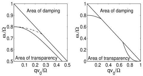
Figure 1: Left panel: Dispersion of the transverse Fermi-liquid cyclotron wave traveling along the external magnetic field for the spherical (dash-dot line) an paraboloidal (solid line) FSs. The curves are plotted using Eqs. (1),(3) assuming $\alpha=-0.2.$ Right panel: A schematic plot of the dispersion of a transverse Fermi-liquid mode in a metal whose FS includes nearly paraboloidal segments. The low frequency $(\omega\ll\Omega)$ branch is shown along with the cyclotron wave. For both panels the straight line corresponds to the Doppler-shifted cyclotron resonance.

This is shown in the Fig. 1 (left panel). However, the dispersion curve meets the boundary of the transparency region at $q=q_{m}\approx 5|\alpha|/3R$ 7 , and at this value of $q$ the dispersion curve is terminated 8 . So, for reasonably weak FL interactions $|\alpha|\sim 0.1$ the Fermi-liquid cyclotron wave may appear only at $qR\ll 1$ and its frequency remains close to the cyclotron frequency for the whole spectrum 9 . Similar conclusions were made using some other models to mimic the FS shape such as an ellipsoid, a nearly ellipsoidal surface and a lens made out of two spherical segments 10 ; 11 .

It is clear that the main contribution to the formation of a weakly attenuated collective mode near the boundary of the transparency region at $\omega\ll\Omega$ comes from those electrons which move with the greatest possible speed along the magnetic field $\bf B.$ The greater is the relative number of such electrons the more favorable conditions are developing for the wave to emerge and to exist at comparatively low frequencies $\tau^{-1}\ll\omega\ll\Omega.$ The relative number of such “efficient” electrons is determined with the FS shape, and the best conditions are reached when the FS includes a lens made out of two paraboloidal cups. Such lens corresponds to the following energy-momentum relation for the relevant conduction electrons:

$$E{\bf(p)}=\frac{{\bf p}^{2}_{\perp}}{2m_{\perp}}+v_{0}|p_{z}|$$ (2)

where $p_{z},\bf p_{\perp}$ are the electron quasimomentum components in the plane perpendicular to the external magnetic field ${\bf B}=(0,0,B),$ and along the magnetic field, respectively. The effective mass $m_{\perp}$ corresponds to electrons motions in the $xy$ plane. This model was employed in some earlier works to study transverse collective modes occuring in a gas of charge carriers near the Doppler-shifted cyclotron resonance which are known as dopplerons 12 ; 13 ; 14 . It was shown 15 that for negative values of the Fermi-liquid parameter $\alpha,$ and provided that the FS contains a paraboloidal segment described by the Eq. (2) the dispersion of the transverse Fermi-liquid wave propagating along the magnetic field has the form $(\tau\to\infty):$

$$\frac{\omega}{\Omega} = 1-\frac{1}{2}(qR+|\alpha|)$$ (3)

$$- \frac{1}{2}\sqrt{(qR-|\alpha|)^{2}+\frac{4}{3}\frac{|\alpha|(qR)^{2}}{qR+\sqrt{(qR)^{2}+|\alpha|^{2}}}}.$$

where $\Omega=eB/m_{\perp}c.$ This result shows that for the paraboloidal FS there are no limitations on frequency of the Fermi-liquid cyclotron wave within the collisionless limit (see Fig. 1, left panel). The only restriction on the wave frequency is caused by the increase of the wave attenuation due to collisions. Taking into account electron scattering one can prove that the wave is weakly attenuated up to a magnitude of the wave vector of the order of $\Omega(1-1/|\alpha|\Omega\tau)/{v_{0}}.$ This value (especially for small $|\alpha|)$ is significantly larger than the value $q_{m}$ for the spherical Fermi surface. Therefore, the frequency of the Fermi-liquid cyclotron waves for negative $\alpha$ can be much smaller than $\Omega$ (remaining greater than $1/\tau$). Comparing the dispersion curves of the transverse Fermi-liquid cyclotron wave for spherical and paraboloidal FSs we see that the FS geometry strongly affects the wave spectrum, and it may provide a weak attenuation of this mode at moderately low frequencies $\omega\ll\Omega.$ In the present work we concentrate on the analysis of the effects of the FS geometry on the occurence of weakly damped Fermi-liquid cyclotron waves propagating in metals along the applied magnetic field at low frequencies $(\tau^{-1}\ll\omega\ll\Omega).$

We show below that in realistic metals with appropriate FSs one may expect a low frequency Fermi-liquid mode to occur along with the Fermi-liquid cyclotron wave as presented in the Fig. 1 (right panel). Both waves have the same polarization, and travel in the same direction. Also, we consider possible manifestations of these low frequency Fermi-liquid waves estimating the magnitude of the corresponding size oscillations in the transmission coeficient for electromagnetic waves propagating through a thin metal film.

II ii. dispersion equation for the transverse Fermi-liquid waves

In the following analysis we restrict our consideration with the case of an axially symmetric Fermi surface whose symmetry axis is parallel to the magnetic field. Then the response of the electron liquid of the metal to an electromagnetic disturbance could be expressed in terms of the electron conductivity circular components $\sigma_{\pm}(\omega,{\bf q})=\sigma_{xx}(\omega,{\bf q})\pm i\sigma_{yx}(\omega,{\bf q}).$ The above restriction on the FS shape enables us to analytically calculate the conductivity components. Also, the recent analysis carried out in Ref. 16 showed that no qualitative difference was revealed in the expressions for the principal terms of the surface impedance computed for the axially symmetric FSs and those not possessing such symmetry, provided that $\bf B$ is directed along a high order symmetry axis of the Fermi surface. This gives grounds to expect the currently employed model to catch main features in the electronic response which remain exhibited when the FSs of generalized (non axially symmetric) shape are taken into consideration.

Within the phenomenological Fermi-liquid theory electron-electron interactions are represented by a self-consistent field affecting any single electron included in the electron liquid. Due to this field the electron energies $E\bf(p)$ get renormalized, and the renormalization corrections depend on the electron position $\bf r$ and time $t:$

$$\Delta E=Tr_{\sigma^{\prime}}\int\frac{d^{3}\bf p^{\prime}}{(2\pi\hbar)^{3}}\,F({\bf p,\hat{\sigma};p^{\prime},\hat{\sigma}^{\prime})\delta\rho(p^{\prime},r,\hat{\sigma}^{\prime},}t).$$ (4)

Here, $\delta\rho{\bf(p,r,\hat{\sigma},}t)$ is the electron density matrix, $\bf p$ is the electron quasimomentum, and $\hat{\sigma}$ is the spin Pauli matrix. The trace is taken over spin numbers $\sigma.$ The Fermi-liquid kernel included in Eq. (4) is known to have a form:

$$F({\bf p,\hat{\sigma};p^{\prime},\hat{\sigma}^{\prime})=\varphi(p,p^{\prime})}+4\bf(\hat{\sigma}\hat{\sigma}^{\prime})\psi(p,p^{\prime})$$ (5)

For an axially symmetric FS the functions $\varphi\bf(p,p^{\prime})$ and $\psi\bf(p,p^{\prime})$ do not vary under identical change in the directions of projections $\bf p_{\perp}$ and $\bf p_{\perp}^{\prime}.$ These functions actually depend only on cosine of an angle $\theta$ between the vectors $\bf p_{\perp}$ and $\bf p_{\perp}^{\prime}$ and on the longitudinal components of the quasimomenta $p_{z}$ and $p_{z}^{\prime}$.

We can separate out even and odd in $\cos\theta$ parts of the Fermi-liquid functions. Then the function $\varphi\bf(p,p^{\prime})$ can be presented as follows:

$$\varphi({\bf p,p^{\prime}})=\varphi_{0}(p_{z},p_{z}^{\prime},\cos\theta)+({\bf p_{\perp}p_{\perp}^{\prime}})\varphi_{1}(p_{z},p_{z}^{\prime},\cos\theta),$$ (6)

where $\varphi_{0},\varphi_{1}$ are even functions of $\cos\theta.$ Due to invariancy of the FS under the replacement $\bf p\to-p$ and $\bf p^{\prime}\to-p^{\prime},$ the functions $\varphi_{0}$ and $\varphi_{1}$ should not vary under simultaneous change in signs of $p_{z}$ and $p_{z}^{\prime}.$ Using this, we can subdivide the functions $\varphi_{0},\varphi_{1}$ into the parts which are even and odd in $p_{z},p_{z}^{\prime},$ and to rewrite Eq. (6) as:

$$\varphi(p_{z},p_{z}^{\prime},\cos\theta)=\varphi_{00}+p_{z}p_{z}^{\prime}\varphi_{01}+({\bf p_{\perp}p_{\perp}^{\prime}})(\varphi_{10}+p_{z}p_{z}^{\prime}\varphi_{11}).$$ (7)

The function $\psi\bf(p,p^{\prime})$ may be presented in the similar way. In the Eq. (7) the functions $\varphi_{00},\varphi_{01},\varphi_{10},\varphi_{11}$ are even in all their arguments, namely: $p_{z},p_{z}^{\prime}$ and $\cos\theta.$

In the following computation of the electron conductivity we employ the linearized transport equation for the nonequilibrium distribution function $g{\bf(p,r,}t)=Tr_{\sigma}(\delta\rho{\bf(p,r,\hat{\sigma},}t)).$ While considering a simple harmonic disturbance ${\bf E=E}_{q\omega}\exp(i{\bf q\cdot r}-i\omega t),$ we may represent the coordinate and space dependencies of the distribution function $g{\bf(p,r,}t)$ as $g{\bf(p,r,}t)=g_{q\omega}\exp(i{\bf qr}-i\omega t).$ Then the linearized transport equation for the amplitude $g_{q\omega}\bf(p)$ takes on the form:

$$\frac{\partial g^{e}_{q\omega}}{\partial\tilde{t}}+i{\bf q\cdot v}g_{q\omega}^{e}+\Big{(}\frac{1}{\tau}-i\omega\Big{)}g_{q\omega}+e\frac{\partial f_{\bf p}}{\partial E_{\bf p}}{\bf vE}_{q\omega}=0.$$ (8)

Here, $f_{\bf p}$ is the Fermi distribution function for the electrons with energies $E\bf(p),$ and ${\bf v}=\partial E/\partial\bf p$ is the electrons velocity. The collision term in the Eq. (8) is written using the $\tau$ approximation which is acceptable for high frequency disturbances $(\omega\tau\gg 1)$ considered in the present work. The derivative $\partial g_{q\omega}^{e}/\partial\tilde{t}$ is to be taken over the variable $\tilde{t}$ which has the meaning of time of the electron motion along the cyclotron orbit. The function $g_{q\omega}^{e}\bf(p)$ introduced in the Eq. (8) is related to $g_{q\omega}\bf(p)$ as follows:

$$g_{q\omega}^{e}{\bf(p)}=g_{q\omega}{\bf(p)}-\frac{\partial f_{\bf p}}{\partial E_{\bf p}}\sum_{\bf p^{\prime}}\varphi{\bf(p,p^{\prime})}g_{q\omega}{\bf(p^{\prime})}.$$ (9)

So, the difference between the distribution functions $g_{q\omega}{\bf(p)}$ and $g_{q\omega}^{e}{\bf(p)}$ originates from the FL interactions in the system of conduction electrons.

Using the transport equation (8) one may derive the expressions for $\sigma_{\pm}(\omega,\bf q)$ including terms originating from the Fermi-liquid interactions. The computational details are given in the Refs. 17 ; 18 . The results for the circular components of the conductivity for a singly connected FS could be written as follows:

$$\begin{array}[]{ll}\sigma_{\pm}=&\displaystyle\frac{2ie^{2}A(0)}{(2\pi\hbar)^{3}q}\\ \\ &\displaystyle\times\frac{\left[\displaystyle\Phi_{0}^{\pm}\Big{(}1-\frac{\alpha_{2}u}{Q_{2}}\Phi_{2}^{\pm}\Big{)}+\frac{\alpha_{2}u}{Q_{2}}(\Phi_{1}^{\pm})^{2}\right]}{\left[\displaystyle\Big{(}1-\frac{\alpha_{1}u}{Q_{0}}\Phi_{0}^{\pm}\Big{)}\Big{(}1-\frac{\alpha_{2}u}{Q_{2}}\Phi_{2}^{\pm}\Big{)}+\frac{\alpha_{1}\alpha_{2}}{Q_{0}Q_{2}}u^{2}(\Phi_{1}^{\pm})^{2}\right]}.\end{array}$$ (10)

Here,

$$\Phi_{n}^{\pm}=\int_{-1}^{1}\frac{\overline{a}(x)\overline{m}_{\perp}(x)x^{n}dx}{u\chi_{\pm}\mp\overline{v}(x)},$$ (11)

$$Q_{n}=\int_{-1}^{1}\overline{a}(x)\overline{m}_{\perp}(x)x^{n}dx.$$ (12)

$$\begin{array}[]{ll}\overline{a}(x)={A(x)}/{A(0)},&\quad\overline{v}(x)={v_{z}}/{v_{0}},\\ \overline{m}_{\perp}(x)={m_{\perp}(x)}/{m_{\perp}(0)},&\quad x={p_{z}}/{p_{0}},\\ \chi_{\pm}=1\pm{\Omega}/{\omega}+{i}/{\omega\tau},&\quad u={\omega}/{qv_{0}}\end{array}$$ (13)

where $v_{0},\ p_{0}$ are the maximum values of longitudinal components of the electron quasimomentum and velocity; $A(x)$ is the FS cross-sectional area; $m_{\perp}(x)$ is the cyclotron mass of electrons. The dimensionless factores $\alpha_{1,2}$ in the Eq. (10) are related to the Fermi-liquid parameters $\varphi_{10}$ and $\varphi_{11}:$

$$\alpha_{1,2}=f_{1,2}\big{/}(1+f_{1,2})$$ (14)

where

$$f_{1}=\frac{2}{(2\pi\hbar)^{3}}\int p_{\perp}^{2}\varphi_{10}m_{\perp}dp_{z},$$

$$f_{2}=\frac{2}{(2\pi\hbar)^{3}}\int p_{\perp}^{2}p_{z}^{2}\varphi_{11}m_{\perp}dp_{z}.$$ (15)

When an external magnetic field is applied, electromagnetic waves may travel inside the metal. In the present work we are interested in the transverse waves propagating along the magnetic field. The corresponding dispersion equation has the form:

$$c^{2}q^{2}-4\pi i\omega\sigma_{\pm}(\omega,{\bf q})=0.$$ (16)

When dealing with the electron Fermi-liquid, this equation for $``-"$ polarization has solutions corresponding to helicoidal waves and the transverse Fermi-liquid waves traveling along the magnetic field. While the relevant charge carriers are holes the $``+"$ polarization is to be chosen in the Eq. (16).

Considering these waves we may simplify the dispersion equation (16) by omitting the first term. Also, we can neglect corrections of the order of $c^{2}q^{2}/\omega_{p}^{2}\ (\omega_{p}$ is the electron plasma frequency) in the expression for the conductivity. Then the Fermi-liquid parameter $\alpha_{1}$ falls out from the dispersion equation, and the latter takes on the form:

$$\Delta(u)=1/\alpha_{2}$$ (17)

where $\Delta(u)=\displaystyle\frac{u}{Q_{2}}\big{[}\Phi_{2}^{-}-(\Phi_{1}^{-})^{2}/\Phi_{0}^{-}\big{]}$.

Assuming the mass $m_{\perp}$ to be the same over the whole FS, and expanding the integrals $\Phi_{n}^{-}$ in powers of $u^{-1}$ and keeping terms of the order of $u^{-2}$ we get the dispersion relation for the cyclotron mode at small $q\ (u\gg 1):$

$$\omega=\Omega(1+f_{2})\bigg{[}1+\frac{\eta}{f_{2}}\bigg{(}\frac{qv_{0}}{\Omega}\bigg{)}^{2}\bigg{]}.$$ (18)

where:

$$\eta=\left[\int_{-1}^{1}\overline{a}(x)\overline{v}^{2}(x)x^{2}dx-\frac{1}{Q_{0}}\left(\int_{-1}^{1}\overline{a}(x)\overline{v}(x)xdx\right)^{2}\right]\frac{1}{Q_{2}}.$$ (19)

For an isotropic electron liquid $\eta=8/35,$ and the expression (18) coincides with the expression (1) where $\alpha=f_{2}.$ Also, adopting the model (2) we may analytically calculate the integrals $\Phi_{n}^{-}$ and to transform the dispersion equation (17) as:

$$3(\chi_{-}+\alpha_{2})(1-(u\chi_{-})^{2})=\alpha_{2}.$$ (20)

At small negative values of the parameter $\alpha_{2}$ this equation has a solution of the form (3) where $\alpha=\alpha_{2}.$

Now, we start to analyze possibilities for the low frequency $(\tau^{-1}\ll\omega\ll\Omega)$ transverse Fermi-liquid mode to emerge in realistic metals where the cyclotron mass depends on $p_{z}.$ Such waves could appear near the Doppler-shifted cyclotron resonance. Assuming $\alpha_{2}<0$ we may describe the relevant boundary of the transparency region by the equations:

$$\left\{\begin{array}[]{l}S(\omega,q,p_{z})=0,\\ \\ {\displaystyle{\partial S(\omega,q,p_{z})}/{\partial p_{z}}=0,}\end{array}\right.$$ (21)

where $S(\omega,q,p_{z})=\omega-\Omega(p_{z})+qv_{z}(p_{z}).$ For small $\omega$ we have

$$\left\{\begin{array}[]{l}{\displaystyle\Omega(p_{z})\left(1+\frac{cq}{2\pi|e|B}\frac{dA}{dp_{z}}\right)=0,}\\ \\ {\displaystyle\frac{d\Omega}{dp_{z}}\left(1+\frac{cq}{2\pi|e|B}\frac{dA}{dp_{z}}\right)+\frac{\Omega(p_{z})cq}{2\pi|e|B}\frac{d^{2}A}{dp_{z}^{2}}=0.}\end{array}\right.$$ (22)

We see that the attenuation at the boundary for small $\omega$ is carried out by the electrons belonging to neighbourhoods of particular cross-sections on the Fermi surface where extrema of the value $dA/dp_{z}$ are reached. These can be neighbourhoods of limiting points or lines of inflection, as shown in the figure 2.

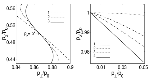
Figure 2: Schematic plots of the FS profiles in the vicinities of inflection lines (left panel) and vertices (right panel). Left panel: The profiles are drawn in accordance with the Eq. (23) assuming $p^{*}=0.5p_{0},\ |d^{s}\overline{a}/dx^{s}|_{x=x^{*}}=|d\overline{a}/dx|_{x=x^{*}}=1,$ and $s=5$ (curve 2), $s=3$ (curve 3). The curve 1 corresponds to a paraboloidal strip on the FS near $x^{*}=0.5\ (s\to\infty).$ Right panel: The curves are plotted asuming $x^{*}=1,\ \overline{a}(1)=0.$ The curves 1 and 4 correspond to a spherical and paraboloidal FSs, respectively; the curves 2,3 represent nearly paraboloidal FSs with $s=7,9$, respectively.

In general, to study various effects in the response of electron liquid of metal near the Doppler-shifted cyclotron resonance one must take into account contributions from all segments of the FS, therefore the expressions for the conductivity components (10) are to be correspondingly generalized. However, in studies of our problem it is possible to separate out that particular segment of the FS where the electrons producing the low frequency Fermi-liquid wave belong. The contribution from the rest of the FS is small, and we can omit it, as shown in Ref. 15 .

So, in the following studies we may use the dispersion equation (17) where the integrals $\Phi_{n}^{\pm}$ are calculated for the appropriate segment of the FS. It follows from this equation that the dispersion curve of the cyclotron wave will not intersect the boundary of the region of transparency when the function $\Delta(u)$ diverges there. A similar analysis was carried out in the theory of dopplerons 14 . It was proven that when the appropriate component of the conductivity (integral of a type of $\Phi_{0}(u))$ goes to infinity at the Doppler-shifted cyclotron resonance, it provides the propagation of the doppleron without damping in a broad frequency range.

In the further analysis we assume for certainty that the extrema of $dA/dp_{z}$ are reached at the inflection lines $p_{z}=\pm p^{*}.$ In the vicinities of these lines we can use the following approximation:

$$\overline{a}(x)\approx\overline{a}(x^{*})+\frac{d\overline{a}}{dx}\bigg{|}_{x=x^{*}}\!\!({x\mp x^{*}})\pm\frac{1}{s!}\frac{d^{s}\overline{a}}{dx^{s}}\bigg{|}_{x=x^{*}}\!\!({x\mp x^{*}})^{s}.$$ (23)

In this expression $x^{*}=p_{z}/p^{*},$ and the parameter $s\ (s\geq 3)$ characterizes the FS shape near the inflection lines at $x=\pm x^{*}.$ The greater is the value of $s$ the closer is the FS near $p_{z}=\pm p^{*}$ to a paraboloid (see Fig. 2). When $s=1$ the FS has spherical/ellipsoidal shape in the vicinities of these points.

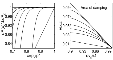
Figure 3: Left panel: Dependencies of $d\overline{a}/dx$ of $x$ near the inflection line on the FS at $x=x^{*}.$ The curves are plotted for $s=4,5,6,7,8,9$ (from the right to the left). Right panel: Dispersion curves of the low frequency transverse Fermi-liquid waves. The curves are plotted at $\alpha_{2}=-0.2;\ s=4,5,6,7,8,$ and $s\to\infty$ (from the top to the bottom) in the collisionless limit assuming that $|d^{s}\overline{a}/d\overline{x}^{s}|_{x=x^{*}}=|d\overline{a}/d\overline{x}|_{x=x^{*}}=1$.

The dependencies of the derivative $d\overline{a}/dx$ of $x$ near $x=x^{*}$ are presented in the left panel of the Fig. 3. In this figure the horizontal line corresponds to a paraboloidal FS $(s\to\infty),$ the straight line on the right is associated with a spherical FS $(s=1)$, and the remaining curves are plotted for $(s>3).$ We can see that the greater is the shape parameter $s$ the broader are nearly paraboloidal strips in the vicinities of the FS inflection lines. Consequently, the greater number of conduction electrons is associated with the nearly paraboloidal parts of the FS, and this creates more favorable conditions for the wave to occur. Similar analysis may be carried out for the case when $dA/dp_{z}$ reachs its extremal values at the vertices of the FS. Again, to provide the emergence of the transverse low frequency Fermi-liquid mode the FS near $p_{z}=\pm p_{0}$ must be nearly paraboloidal in shape.

Using the asymptotic expression (23) we may calculate the main term in the function $\Delta(u).$ This term diverges at the boundary of the region of transparency when $s\geq 3,$ and it has the form:

$$\Delta_{-}(u)=-\nu_{s}u(1-u\chi_{-})^{\mu_{s}}$$ (24)

where $\mu_{s}=(5-2s)/(2s-2).$ For $s>3,\ \mu_{s}$ takes on negative values, so within the collisionless limit $(\tau\to\infty)$ the function $\Delta_{-}(u)$ diverges when $1-u\chi_{-}\to 0.$ The value of the factor $\nu_{s}$ is determined with the FS geometry near the inflection line, namely:

$$\nu_{s}=\frac{\pi\overline{a}(x^{*})\overline{m}_{\perp}(x^{*})\zeta_{s}}{Q_{2}(s-1)\sin[3\pi/(2s-2)]}$$ (25)

where

$$\zeta_{s}=\left(\frac{|d^{s}\overline{a}/dx^{s}|_{x=x^{*}}}{(s-1)!|d\overline{a}/dx|_{x=x^{*}}}\right)^{-3/2(s-1)}.$$ (26)

Now, we can employ the approximation (24) to solve the dispersion equation (17). The solutions of this equation within the collisionless limit describing the low frequency transverse Fermi-liquid wave at different values of the shape parameter $s$ are plotted in the figure 3 (right panel). All dispersion curves are located in between the boundary of the transparency window and the straight line corresponding to the limit $s\to\infty$ (a paraboloidal FS). The greater is the value of $s$ the closer is the dispersion curve to this line.

So, we showed that the low frequency $(\omega\ll\Omega)$ transverse Fermi-liquid wave could appear in a metal put into a strong $(\Omega\tau\gg 1)$ magnetic field. This could happen when the FS is close to a paraboloid near those cross-sections where $dA/dp_{z}$ reachs its maxima/minima. Therefore, the possibility for this wave to propagate in a metal is provided with the local geometry of the Fermi surface near its inflection lines or vertices.

When $\Omega$ depends on $p_{z}$ and $\omega$ increases, electrons associated with various cross-sections of the Fermi surface participate in the formation of the wave. To provide the divergence of the function $\Delta(u)$ near the Doppler-shifted cyclotron resonance we have to require that not merely narrow strips near lines of inflection or vicinities of limiting points but rather large segments of the Fermi surface are nearly paraboloidal. This condition is too stringent for FSs of real metals. So, we can expect that the dispersion curve of the low frequency transverse Fermi-liquid wave intersects the boundary of the region of transparency at rather small $\omega,$ as shown in the right panel of the Fig. 1.

III iii. size oscillations in the surface impedance

To clarify possible manifestations of the considered Fermi-liquid wave in experiments we calculate the contribution of these waves to the transmission coefficient of a metal film. We assume that the film occupies the region $0\ll z\leq L$ in the presence of an applied magnetic field directed along a normal to the interfaces. An incident electromagnetic wave with the electric and magnetic components ${\bf E}(z)$ and ${\bf b}(z)$ propagates along the normal to the film. Also, we assume that the simmetry axis of the FS is parallel to the magnetic field $(z$-axis) and the interfaces reflect the conduction electrons in a similar manner. Then the Maxwell equations inside the metal are reduced to the couple of independent equations for circular components of the electrical field $E_{\pm}(z)\exp(-i\omega t)$ where $(E_{\pm}=E_{x}\pm iE_{y}):$

$$\frac{\partial^{2}E_{\pm}}{\partial z^{2}}=-\frac{\omega^{2}}{c^{2}}E_{\pm}(z)-\frac{4\pi i\omega}{c^{2}}j_{\pm}(z),$$ (27)

$$\frac{\partial E_{\pm}(z)}{\partial z}=\mp\frac{\omega}{c}b_{\pm}(z).$$ (28)

Here, $b_{\pm}(z)$ and $j_{\pm}(z)$ are the magnitudes of the magnetic component of the incident electromagnetic wave and the electric current density inside the film, respectively. Expanding the magnitudes $E_{\pm}(z)$ and $j_{\pm}(z)$ in Fourier series we arrive at the following equation for the Fourier transforms:

$$-\frac{c^{2}q_{n}^{2}}{4\pi i\omega}E_{n}^{\pm}+j_{n}^{\pm}=\mp\frac{ic}{4\pi}[(-1)^{n}b_{\pm}(L)-b_{\pm}(0)]$$ (29)

where $E_{n}^{\pm}$ equals:

$$E_{n}^{\pm}=\int_{0}^{L}E_{\pm}(z)\cos(q_{n}z)dz$$ (30)

and $q_{n}=\pi n/L.$

It was mentioned above that possible frequencies of the low frequency Fermi-liquid mode have to satisfy  the inequality $(|\alpha_{2}|\tau)^{-1}\ll\omega<\Omega.$ For $\tau<10^{-9}$s the frequency $\omega$ can not be lower than $10^{9}\div 10^{10}$s${}^{-1}.$ Due to high density of conduction electrons in good metals the skin depth $\delta$ may be very small. Assuming the electron density to be of the order of $10^{30}$m^-3, and the mean free path $l\sim 10^{-5}$m (a clean metal), we estimate the skin depth at the disturbance frequency $\omega\sim 10^{9}$s^-1 as $\delta\sim 10^{-6}$m. Therefore, at high frequencies $\omega$ the skin effect in good metals becomes extremely anomalous so that $\delta/l\sim 10^{-1}\div 10^{-2}$ or even smaller. Correspondingly, the anomaly parameter $\xi=l/\omega\tau\delta$ is of the order $10^{2}\div 10^{3}.$ Thus, for all frequency range of the considered Fermi-liquid mode the skin effect is of anomalous character. Under these conditions electrons must move nearly in parallel with the metal surface to remain in the skin layer for a sufficiently long while. The effect of the surface roughness on such electrons is rather small. Nevertheless, we may expect the effects of surface roughness to bring changes in the corresponding size oscillations of the transmission coefficient. To take into account the effects of diffuse scattering of electrons from the surfaces of the film one must start from the following expression for the Fourier transforms of the current density components:

$$j_{n}^{\pm}=\sigma_{n}^{\pm}E_{n}^{\pm}+\sum_{n^{\prime}=0}\left(1-\frac{1}{2}\delta_{n^{\prime}0}\right)\sigma_{nn^{\prime}}^{\pm}E_{n^{\prime}}^{\pm}$$ (31)

where $\sigma_{n}^{\pm}=\sigma_{xx}(\omega,q_{n})\pm i\sigma_{yx}(\omega,q_{n})$ are the circular components of the bulk conductivity, and $\sigma_{nn^{\prime}}=\sigma_{xx}(\omega,q_{n},q_{n^{\prime}})\pm\sigma_{yx}(\omega,q_{n},q_{n^{\prime}})$ are the circular components of the surface conductivity. The effects originating from the surface roughness are included in $\sigma_{nn^{\prime}}^{\pm}$ which becomes zero for a smooth surface providing the specular reflection of electrons. The calculation of $\sigma_{nn^{\prime}}^{\pm}$ is a very difficult task which could hardly be carried out analytically if one takes into account Fermi-liquid correlations of electrons. However, such calculations were performed for a special case of paraboloidal FS corresponding to the energy-momentum relation (2) in the earlier work 19 . As was mentioned before, the FS segments which give the major contributions to the formation of the transverse Fermi-liquid mode are nearly paraboloidal in shape, therefore the results of the work 19 may be used to qualitatively estimate the significance of the surface scattering of electrons under the conditions of the anomalous skin effect. We assume for simplicity that the diffuse scattering is characterized by a constant $P\ (0<P<1).$ When $P=0,$ the reflection of electrons is purely specular, whereas $P=1$ corresponds to the completely diffuse reflection. Adopting the expression (2) to describe electrons spectrum one could obtain:

$$\sigma_{n}^{\pm} = \pm\frac{iNe^{2}}{3m_{\perp}\omega}\chi_{\pm}\left(\frac{1}{\theta_{n}^{\pm}}+\frac{2(\chi_{\pm}^{*}/\chi_{\pm})^{2}}{\theta_{n}^{*\pm}}\right),$$ (32)

$$\sigma_{nn^{\prime}}^{\pm} = \frac{4}{3}\frac{Ne^{2}}{m_{\perp}\omega}\lambda\frac{v_{0}}{\omega L}\chi_{\pm}^{2}\left(\frac{1}{1\mp\lambda s_{\pm}}\frac{1}{\theta_{n}^{\pm}\theta_{n^{\prime}}^{\pm}}\right.$$ (33)

$$+\left.\frac{2(\chi_{\pm}^{*}/\chi_{\pm})^{4}}{1\mp\lambda s_{\pm}^{*}\chi_{\pm}^{*}/\chi_{\pm}}\frac{1}{\theta_{n}^{*\pm}\theta_{n^{\prime}}^{*\pm}}\right)$$

where $N$ is the electrons density,

$$\begin{array}[]{l}s_{\pm}=i\tan(L\Omega\chi_{\pm}/v_{0}),\quad s_{\pm}^{*}=i\tan(L\Omega\chi_{\pm}^{*}/v_{0}),\\ \theta_{n}^{\pm}=\chi_{\pm}^{2}-q_{n}^{2},\\ \theta_{n}^{*\pm}=\chi_{\pm}^{*2}-q_{n}^{2}\equiv\chi_{\pm}^{2}\mp\alpha_{2}\chi_{\pm}-q_{n}^{2}.\\ \end{array}$$ (34)

The parameter $\lambda=P/(2-P)$ characterizes the strength of the diffuse component in the electron scattering from the surfaces of the metal film.

Comparing the expressions (32) and (33) we conclude that $\sigma_{n}^{\pm}$ predominates over $\sigma_{nn^{\prime}}$ in magnitude when $\lambda\xi\delta/L\ll\omega/\Omega.$ Assuming that the anomaly parameter $\xi\sim 10^{2},$ the skin depth $\delta\sim 10^{-6}$m, and $\omega\sim\Omega$ we conclude that the roughness of the surface does not affect the transmission coefficient if the film thickness $L$ is not smaller than $10^{-4}$m. For thinner films the surface roughness may bring noticeable changes into the transmission. For instance, when $L\sim l\sim 10^{-5}$m, we may neglect the diffuse contribution to the electrons reflection at the surfaces of the film when $\lambda<0.1\ (P<0.2).$ In further calculations we assume the film surfaces to be smooth enough, so that we could treat the electrons reflection from the metal film surfaces as nearly specular. Correspondingly, we omit the second term in the expression (31).

Substituting the resulting expressions for $j_{n}^{\pm}$ into Eq. (29) we get:

$$E_{n}^{\pm}=\mp\frac{\omega}{c}F_{\pm}(\omega,q_{n})[(-1)^{n}b_{\pm}(L)-b_{\pm}(0)].$$ (35)

Here, we introduced the notation:

$$F_{\pm}(\omega,q_{n})=\left(q_{n}^{2}-\frac{4\pi i\omega}{c^{2}}\sigma_{n}^{\pm}\right)^{-1}.$$ (36)

Now, using these expressions for the Fourier transforms we get the relations for the electric and magnetic fields at the interfaces $z=0$ and $z=L:$

$$E_{\pm}(0)=\frac{c}{4\pi}\left[Z_{\pm}^{(0)}b_{\pm}(0)-Z_{\pm}^{(1)}b_{\pm}(L)\right],$$ (37)

$$E_{\pm}(0)=\frac{c}{4\pi}\left[Z_{\pm}^{(1)}b_{\pm}(0)-Z_{\pm}^{(0)}b_{\pm}(L)\right],$$ (38)

where the surface impedances are given by:

$$Z_{\pm}^{(0)}\! = \!\pm\frac{8\pi\omega}{Lc^{2}}\sum_{n=0}\left(1-\frac{1}{2}\delta_{n0}\right)F_{\pm}(\omega,q_{n}),$$ (39)

$$Z_{\pm}^{(1)}\! = \!\pm\frac{8\pi\omega}{Lc^{2}}\sum_{n=0}\left(1-\frac{1}{2}\delta_{n0}\right)(-1)^{n}F_{\pm}(\omega,q_{n}).$$ (40)

To get the expression for the transmission coefficient which is determined by the ratio of the amplitudes of the transmitted field $(E_{t})$ at $z=L$ and the incident field $(E_{i})$ at $z=0$ we use the Maxwell boundary conditions:

$$2E_{i}^{\pm}=E_{\pm}(0)+b_{\pm}(0),\qquad E_{t}^{\pm}=b_{\pm}(L).$$ (41)

Then we define $T_{\pm}=\big{|}E_{t}^{\pm}/E_{i}^{\pm}\big{|}$ where $E_{t}^{\pm}/E_{i}^{\pm}=[E_{\pm}(L)+b_{\pm}(L)]/[E_{\pm}(0)+b_{\pm}(0)].$ Assuming that the transmission is small $(T_{\pm}\ll 1)$ we get the asymptotic expression:

$$\frac{E_{t}^{\pm}}{E_{i}^{\pm}}\approx\frac{c}{4\pi}Z_{\pm}^{(1)}$$ (42)

where $Z_{\pm}^{(1)}$ is given by the relation (40).

Therefore, keeping the $``-"$ polarization we can start from the following expression for the transmission coefficient:

$$T=\frac{4i\omega}{Lc}\sum_{n=0}(-1)^{n+1}\left(1-\frac{1}{2}\delta_{n0}\right)F_{-}(\omega,q_{n}),$$ (43)

Using the Poisson’s summation formula:

$$\sum_{n=0}y(q_{n})=\sum_{r=-\infty}^{\infty}\int_{0}^{\infty}y\left(\frac{\pi}{L}x\right)\exp(2\pi irx)dx,$$ (44)

we convert the expression for the transmission coefficient to the form:

$$T=\frac{2}{\pi}\frac{\omega}{c}\int_{-\infty}^{\infty}\mbox{sign}(q)\mbox{cosec}(Lq)F_{-}(\omega,q)dq.$$ (45)

where $\mbox{sign}(q)$ it the sign function: $\mbox{sign}(q)=|q|/q.$ An important contribution to the integral (45) comes from the poles of the function $F_{-}(\omega,q),$ i.e. the roots of the dispersion equation (16) for the relevant polarization. The contribution from the considered low frequency mode to the transmission coefficient is equal to a residue from the appropriate pole of the integrand in the expression (45).

When $dA/dp_{z}$ gets its extremal values at the inflection lines $(p_{z}=\pm p^{*})$ the contribution $T_{1}$ from this wave to the transmission coefficient is:

$$T_{1}\! \approx \!\frac{\rho_{s}}{\xi}\frac{v_{0}}{c}\alpha_{2}^{2}\tilde{\omega}^{3}(|\alpha_{2}|\tilde{\omega})^{-7s/2}(1-\tilde{\omega})^{-3/(2s-5)}$$ (46)

$$\!\times\left[\sin^{2}\left(\frac{L}{l}\Omega\tau(1-\tilde{\omega})\right)+\sinh^{2}\left(\frac{L}{l}\right)\right]^{-1/2}$$

where $\tilde{\omega}=\omega/\Omega(p^{*}),$ and $\rho_{s}$ is the dimensionless factor of the order of unity:

$$\rho_{s}=\frac{2s-3}{2s-5}\,\frac{Q_{0}}{Q_{2}}(x^{*})^{2}(\nu_{s})^{(2s-3)/(2s-5)}$$ (47)

The size oscillations of the transmission coefficient arising due to the low frequency cyclotron wave could be observed in thin films whose thickness is smaller than the electrons mean free path $(L\ll l).$ Under this condition we can obtain the following estimates for $|T_{1}|$ in a typical metal in a magnetic field of the order of $5T$, and for the shape parameter $s=3:$

$$T_{1}\sim\left(10^{-10}\div 10^{-11}\right)l/L.$$ (48)

Size oscillations of the transmission coefficient described by the expression (43) are shown in the figures 4,5. When $(s=3)$ (see Fig. 4) the oscillations amplitudes accept values $\sim 10^{-8}\div 10^{-9}$ depending on the ratio $L/l.$ The values of such order can be measured in experiments on the transmission of electromagnetic waves through thin metal films. However, the oscillations magnitudes may reach significantly greater values when the shape parameter increases. As displayed in the Fig. 5, $T_{1}$ can reach the values of the order of $10^{-6}$ when $s=5.$

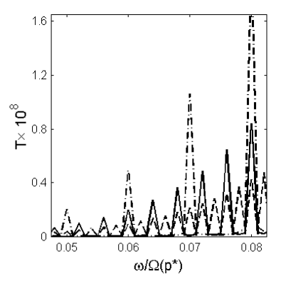
Figure 4: Size oscillations in the transmission coefficient for the transverse electromagnetic wave traveling through a metal film which originate from the low frequency Fermi-liquid mode. The curves are plotted at $\alpha_{2}=-0.2,\ s=3.\ \Omega\tau\sim 50,\xi=10^{3},\ L/l=0.01$ (dash-dot line); $0.025$ (solid line) and $0.05$ (dashed line).

Under considered conditions the transmission coefficient also includes a contribution $T_{2}$ from electrons corresponding to the vicinities of those cross-sections of the Fermi surface where the longitudinal component of their velocity becomes zero. This contribution always exists under the anomalous skin effect. The most favorable conditions for observation of the size oscillations arising due to the Fermi-liquid wave in experiments are provided when $T_{1}>T_{2}.$ It happens when $L\omega\xi>v_{0}.$ When the FS everywhere has a finite nonzero curvature the expression for $T_{2}$ can be written as follows 20 :

$$T_{2}\approx\frac{4}{3}\frac{v_{0}}{c}\frac{1}{\xi}\exp\left(-\frac{L\omega\tau\xi}{l}\right);$$ (49)

In magnetic fields $\sim 5T$ and for $L\omega\sim v_{0}$ the contribution $T_{2}$ has the order of $10^{-10}\div 10^{-11},$ i.e. the predominance of the term $T_{1}$ over $T_{2}$ can be reached. Besides the contributions from the poles of $F_{-}(\omega,q)$ the transmission coefficient (45) includes a term $T_{3}$ originating from the branch points of this function in the $q,\omega$ complex plane. These points cause the Gantmakher–Kaner size oscillations of the transmission coefficient 21 . However, for $L\Omega>v_{0},$ these oscillations have a magnitude of the order of $10^{-9}\div 10^{-10}$ or less. So, the present estimates give grounds to expect that the size oscillations in the transmission coefficient of the electromagnetic wave through a thin film of a clean metal may include a rather significant, or even predominating contribution, which arises due to the low frequency $(\omega\ll\Omega)$ Fermi-liquid mode.

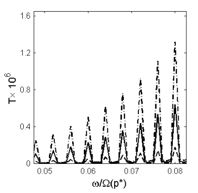
Figure 5: The dependence of the transmission from the FS shape near the inflection line. The curves are plotted for $s=3$ (dashed line), 4 (solid line) and 5 (dash-dot line), $L/l=0.025.$ The remaining parameters coincide with those used to plot the curves in the figure 4.

Fermi surfaces of real metals are very complex in shape and most of them have inflection lines, so there are grounds to expect the low frequency Fermi-liquid waves to appear in some metals. Especially promising are such metals as cadmium, tungsten and molybdenium where collective excitations near the Doppler-shifted cyclotron resonance (dopplerons) occur 12 ; 13 ; 14 . Another kind of interesting substances are quasi-two-dimensional conductors. Applying the external magnetic field along the FS axis and using the tight-binding approximation for the charge carriers, we see that the maximum longitudinal velocity of the latter is reached at the FS inflection lines where $d^{2}A/dp_{z}^{2}=0.$ So, we may expect the low frequency Fermi-liquid wave to appear at some of these substances along with the usual Fermi-liquid cyclotron wave.

IV iv. conclusion

It is a common knowledge that electron-electron correlations in the system of conduction electrons of a metal may cause occurences of some collective excitations (Fermi-liquid modes), whose frequencies are rather close to the cyclotron frequency at strong magnetic fields $(\Omega\tau\gg 1)$. Here we show that a Fermi-liquid wave can appear in clean metals at significantly lower frequencies $(\tau^{-1}\ll\omega\ll\Omega).$ The major part in the wave formation is taken by the electrons (or holes) which move along the applied magnetic field with the maximum velocity $v_{0}.$ Usually, such electrons belong to the vicinities of limiting points or inflection lines on the FS. When the FS possesses nearly paraboloidal segments including these points/lines, the longitudinal velocity of the charge carriers slowly varies over such FS segments remaining close to its maximum value $v_{0}.$ This strengthens the response of these “efficient” electrons to the external disturbances. As a result the spectrum of the Fermi-liqud cyclotron wave may be significantly changed. These changes were analyzed in some earlier works (see e.g. Ref. 15 ) assuming that the cyclotron mass of the charge carriers remains the same all over the FS. Under this assumption it was shown that the appropriate FS geometry at the segments where the maximum longitudinal velocity of electrons/holes is reached may cause the dispersion curve of the transverse Fermi-liquid cyclotron wave to be extended to the region of comparatively low frequencies $(\omega\ll\Omega).$

In the present work we take into account the dependence of cyclotron mass of $p_{z}.$ This more realistic analysis leads to the conclusion that one hardly may expect the above extension of the Fermi-liquid cyclotron wave spectrum in real metals. However, when the FS has the suitable geometry at the segments where the charge carriers with maximum longitudinal velocity are concentrated, the low frequency Fermi-liquid mode may occur in the metal alongside the usual Fermi-liquid cyclotron wave. This mode may cause a special kind of size oscillations in the transmission coefficient for an electromagnetic wave of the corresponding frequency and polarization incident on a thin metal film.

V Acknowledgments

The author thanks G. M. Zimbovsky for help with the manuscript. This work was supported by NSF Advance program SBE-0123654, DoD grant W911NF-06-1-0519, and PR Space Grant NGTS/40091.

References

• (1) A. A. Abrikosov, Foundations of the Theory of Metal (North-Holland, Amsterdam, 1988).
• (2) P. M. Platzman and P. A. Wolff, Waves and Interactions in Solid State Plasma (Academic, New York, 1973).
• (3) E. A. Kaner and V. G. Skobov, Advances in Phys. 17, 605 (1968).
• (4) V. P. Silin, Zh. Eksp. Teor. Fiz. 33, 1227 (1958) [Sov. Phys. JETP 6, 1945 (1958)].
• (5) S. Schultz and G. Dunifer, Phys. Rev. Lett. 18, 283 (1967).
• (6) P. M. Platzman, W. Walsh, and E-Ni Foo, Phys. Rev. 172, 689 (1968).
• (7) Y. C. Cheng, J. S. Clarke and D. Merminn, Phys. Rev. Lett. 20, 1486 (1968).
• (8) At $q>q_{m}$ the wave is damped by the conduction electrons.
• (9) J. J. Quinn and S. C. Ying, Phys. Rev. 180, 1283 (1970).
• (10) T. P. Alodzhantz, Zh. Eksp. Teor. Fiz. 59, 1429 (1970) [Sov. Phys. JETP 32, 780 (1971)].
• (11) Y. C. Cheng, Phys. Rev. B 3, 2287 (1973).
• (12) S. V. Lavrova, V. T. Medvedev, V. G. Skobov, L. M. Fisher, and A. S. Chernov, Zh. Eksp. Teor. Fiz. 64, 1839 (1973) [Sov. Phys. JETP 37, 929 (1973)].
• (13) V. T. Medvedev, V. G. Skobov, L. M. Fisher, and V. A. Yudin, Zh. Eksp. Teor. Fiz. 69, 2267 (1975) [Sov. Phys. JETP 42, 1152 (1975)].
• (14) D. S. Folk, B. Gerson, and J. F. Carolan, Phys. Rev. B 1, 406 (1970).
• (15) N. A. Zimbovskaya, V. I. Okulov, A. Yu. Romanov, and V. P. Silin, Fiz. Nizk. Temp. 8, 930 (1982) [Soviet J. Low Temp. Phys. 8, 468 (1982)].
• (16) N. A. Zimbovskaya and G. Gumbs, Phys. Rev. B 72, 045112 (2005).
• (17) O. V. Kirichenko, V. G. Peschansky, and D. I. Stepanenko, Phys. Rev. B 71, 045304 (2005).
• (18) N. A. Zimbovskaya, Phys. Rev. B 74, 035110 (2006).
• (19) N. A. Zimbovskaya, V. I. Okulov, A. Yu. Romanov, and V. P. Silin, Fiz. Met. Metalloved. 58, 851 (1984)[In Rissian].
• (20) N. A. Zimbovskaya and V. I. Okulov, Fiz. Met. Mettaloved. 61, 230 (1986) [In Russian].
• (21) V. F. Gantmakher and E. A. Kaner, Zh. Eksp. Teor. Fiz. 48, 1572 (1965) [Sov. Phys. JETP 21, 1053 (1965)].