THE DIFFERENTIAL ROTATION OF $\kappa^{1}$ CETI AS OBSERVED BY MOST  – II

Abstract

We first reported evidence for differential rotation of $\kappa^{1}$ Ceti in Paper I. In this paper we demonstrate that the differential rotation pattern closely matches that for the Sun. This result is based on additional MOST (Microvariability & Oscillations of STars) observations in 2004 and 2005, to complement the 2003 observations discussed in Paper I. Using StarSpotz, a program developed specifically to analyze MOST photometry, we have solved for $k$, the differential rotation coefficient, and $P_{EQ}$, the equatorial rotation period using the light curves from all three years. The spots range in latitude from 10^∘ to 75^∘ and $k$ = $0.090^{+0.006}_{-0.005}$ – less than the solar value but consistent with the younger age of the star. $k$ is also well constrained by the independent spectroscopic estimate of $v$sin$i$. We demonstrate independently that the pattern of differential rotation with latitude in fact conforms to solar.

Details are given of the parallel tempering formalism used in finding the most robust solution which gives $P_{EQ}$ = $8.77^{+0.03}_{-0.04}$  days – smaller than that usually adopted, implying an age $<$ 750 My. Our values of $P_{EQ}$ and $k$ can explain the range of rotation periods determined by others by spots or activity at a variety of latitudes. Historically, Ca II activity seems to occur consistently between latitudes 50^∘ and 60^∘ which might indicate a permanent magnetic feature. Knowledge of $k$ and $P_{EQ}$ are key to understanding the dynamo mechanism and rotation structure in the convective zone as well assessing age for solar-type stars. We recently published values of $k$ and $P_{EQ}$ for $\epsilon$ Eri based on MOST photometry and expect to analyse MOST light curves for several more spotted, solar-type stars.

1. INTRODUCTION

Differential rotation and convection provide the engine for the solar dynamo (eg. Ossendrijver (2003)). The mechanism suggested by Lebedinskii (1941) for differential rotation seems to be the most widely accepted. Angular momentum is continually redistributed in the deep convective envelope which occupies some 30% of the outer solar radius resulting in nonuniform rotation because the convective turbulence is affected by the Coriolis force (Kitchatinov, 2005). There is good evidence that a younger Sun would have rotated more rapidly and gradually lost angular momentum through magnetic coupling to the solar wind and there is currently a considerable theoretical effort to develope quantitative models of differential rotation in solar-type stars (see, for example, reviews by Kitchatinov (2005) and Thompson et al. (2003)).

For stars other than the Sun, the simultaneous detection of two or more spots at different latitudes allows a direct measurement of differential rotation. The MOST photometric satellite (Walker et al., 2003a) offers continuous photometry of target stars with an unprecedented precision for weeks at a time making it it possible to track spots accurately.

We (Rucinski et al., 2004) have already reported the detection of a pair of spots in the 2003 MOST light curve of $\kappa^{1}$ Ceti (HD 20630, HIP 15457, HR 996; $V=4.83$, $B-V=0.68$, G5V). The photometry was part of the satellite commissioning and prior to a considerable improvement pointing in early 2004. The larger spot had a well-defined 8.9 d rotation period while the smaller one had a period $\geq$9.3 d. Only the latitude of the larger spot could be determined with any confidence. Spectroscopic observations by Shkolnik et al. (2003), mostly from 2002, of the Ca II K-line emission reversals were also synchronized to a period of about 9.3 d. Rucinski et al. (2004) also determined a stellar radii of $R_{*}$ = 0.95 $\pm$ 0.10 $R_{\bigodot}$.

To better decipher the spot activity and rotation of ${\kappa}^{1}$ Ceti and to model spot distributions on other MOST targets, one of us, BC, developed the program Starspotz (Croll et al. (2006b); Croll (2006a)). It was applied first to a 2005 MOST light curve covering three rotations of $\epsilon$ Eri where two spots were detected at different latitudes rotating with different periods. From this, we derived a differential rotation coefficient for $\epsilon$ Eri (see section 4), $k=0.11^{+.03}_{-.02}$, in agreement with models by Brown et al. (2004) for young Sun-like stars rotating roughly twice as fast as the Sun.

In this paper, we apply Starspotz to the three separate MOST light curves of $\kappa^{1}$ Ceti – from 2003, 2004 and 2005. We specifically solve for the astrophysically important elements of inclination, differential rotation, equatorial period and rotation speed and find that the differential rotation profile is identical to solar.We use parallel tempering methods to fully explore the realistic parameter space and identify the global $\chi^{2}$ minimum to the data-set that signifies a best-fitting unique starspot configuration. Markov Chain Monte Carlo (MCMC) methods are then used to explore in detail the parameter space around this global minimum, to define best-fitting values and their uncertainties and to explore possible correlations among the fitted and derived parameters.

2. MOST PHOTOMETRY AND LIGHT CURVES

The MOST satellite, launched on June 2003, is fully described by Walker et al. (2003a). A 15/17.3 cm Rumak-Maksutov telescope feeds two CCDs, one for tracking and the other for science, through a single, custom, broadband filter (350 – 700 nm). Starlight from primary science targets ($V\leq 6$) is projected onto the science CCD as a fixed (Fabry) image of the telescope entrance pupil covering some 1500 pixels. The experiment was designed to detect photometric variations with periods of minutes at micro-magnitude precision and does not use comparison stars or flat-fielding for calibration. There is no direct connection to any photometric system. Tracking jitter was dramatically reduced early in 2004 to $\sim$1 arcsec which, subsequently, led to significantly higher photometric precision.

The observations reported here were reduced by RK. Outlying data points generated by poor tracking or cosmic ray hits were removed. At certain orbital phases, MOST suffers from parasitic light, mostly Earthshine, the amount and phase depending on the stellar coordinates, spacecraft roll and season of the year. Data are recorded for seven Fabry images adjacent to the target to track the background. The background signals were combined in a mean and subtracted from the target photometry. This procedure also corrected for bias, dark and background signals and their variations. Reductions basically followed the scheme already outlined by Rucinski et al. (2004).

Table 1MOST Observations of $\kappa^{1}$ Ceti

year	dates	total	duty cycle	exp	cycle	$\sigma$
start	HJD – 2451545	days	%	sec	sec	mmag
2003  5 Nov	1403.461 to 1433.901	30.44	96	40	50	0.5
2004 15 Oct	1748.578 to 1768.989	20.41	99	30	35	0.30
2005 14 Oct	2112.721 to 2125.065	12.34	83	30	35	0.19

A log of the MOST observations of $\kappa^{1}$ Ceti for each of 2003, 2004 and 2005 is given in Table 1. For the light curve analysis in this paper, data were binned at the MOST orbital period of 101.413 min. Figure 1 displays full light curves for each of the three years with time given as JD-2451545 (heliocentric). The solid line in the lower panel displays the difference between the two most divergent background readings from the seven background Fabry images. There is no obvious correlation between structure in the differential background signal and the light curve. The complete light curve can be downloaded from the MOST Public Archive at www.astro.ubc.ca/MOST.

The formal rms point-to-point precison, $\sigma$, is given in Table 1. The shapes of the light curves ultimately used for the StarSpotz analysis depend to a degree on just how the background is removed. Despite having the summed signal values from 7 adjacent Fabry images we cannot interpolate a ‘true’ background but subtraction of the mean background is a consistent option. In each of the three data sets used here the 7 background values are closely identical when averaged over an orbit but the differences between the extreme backgrounds can be significant when the ambient background is high (eg. pointing close to the Moon) which is why that difference is shown in the lower panel for each light curve.

We have assumed that the true errors in the individual orbital means making up each light curve are proportional to the difference between the maximum and minimum background values. These errors have been arbitrarily scaled by one-fourth for the formal StarSpotz analysis and these ‘errors’ are shown as bars in Figures 4, 5, and 6. The individual bars correspond approximately to the standard deviation of the background.

3. StarSpotz

StarSpotz (Croll et al., 2006b) is a program based on SPOTMODEL (Ribárik et al. 2003; Ribárik 2002), that is designed to provide a graphical user interface for photometric spot modeling. The functionality included in StarSpotz is designed to take advantage of the nearly continuous photometry returned by MOST to quantify the non-uniqueness problem often associated with photometric spot modeling. Basically, StarSpotz uses the analytic models of Budding (1977) or Dorren (1987) to model the drop in intensity caused by $N_{SPOT}$ circular, non-overlapping spots. The model proposed in Budding (1977) is used in this application.

Fitting can be performed by a variety of methods including a Marquardt-Levenberg non-linear least squares algorithm (Marquardt 1963; Levenberg 1944; Press et al. 1992), or Markov Chain Monte Carlo (MCMC) functionality (Gregory 2005b; Gamerman et al. 1999; Gilks et al. 1996). The parameters of interest are the stellar inclination angle, $i$, the unspotted intensity of the star, $U$, and the period, epoch, latitude and angular size of the $a^{th}$ spot: $p_{a}$, $E_{a}$, $\beta_{a}$, and $\gamma_{a}$. Croll et al. (2006b) have demonstrated how the Marquardt-Levenberg non-linear least squares algorithm could be used to fit the cycle to cycle variation in $\epsilon$ Eri. Croll (2006a) investigated the same observations of $\epsilon$ Eri demonstrating that Markov Chain Monte Carlo functionality is very helpful in defining correlations and possible degeneracies between the fitted parameters.

The search for additional local minima in $\chi^{2}$ space indicating other plausible spot configurations that produce a reasonable fit to the light-intensity curve is an important part of the modeling because it allows one to quantify the uniqueness of a solution. We argue that this task of completely searching parameter space for other physically plausible local minima is better suited to a process called parallel tempering (Gregory 2005a; Gregory 2005b), discussed here in $\S$4.2, rather than the Uniqueness test methods in Croll et al. (2006b).

The present and subsequent releases of the freely available program StarSpotz, including the full source-code, executable, and documentation are available at:

www.astro.ubc.ca/MOST/StarSpotz.html

Release 3.0 includes the functionality discussed which allows one to fit multiple epochs of data as well as the parallel tempering functionality.

4. The Spots on $\kappa^{1}$ Ceti

As the MOST observations of $\kappa^{1}$ Ceti come from three well-seperated epochs with independent starspot groups from epoch to epoch, the fitting process was considerably more complicated than those detailed in Croll et al. (2006b) and Croll (2006a). Rather than fitting for the period, $p$, of the individual spots in each epoch we derive a common equatorial period, $P_{EQ}$, and the differential rotation coefficient, $k$, among the three epochs where these are given by:

$$P_{\beta}=P_{{\rm EQ}}/(1-k~{}{\rm sin}^{2}\beta)$$ (1)

where $P_{\beta}$ is the period at latitude $\beta$. There are five fewer parameters to be fitted because the periods of the individual spots are no longer independent variables, but completely defined by $k$, $P_{EQ}$, and $\beta$. Analyses of solar differential rotation usually include terms in sin${}^{4}\beta$ (Kitchatinov, 2005) but we did not expect to detect spots at such high latitudes where this term would be important.

Common limb-darkening coefficients, $u$ = 0.684, and flux ratios between the spot and unspotted photosphere, $\kappa_{\omega}$ = 0.22 were assumed. The former was based on the compilations of Díaz-Cordovés et al. (1995), while the latter comes from the canonical value for sunspots ($T_{spot}\sim 4000$ K, $T_{phot}\sim 5800$ K). The 27 parameters to be fitted are summarized in Table 2.

Initial investigations of the light curves using the StarSpotz standard spot model indicated that different numbers of spots were required for the various epochs. The 2003 and 2005 MOST data-sets could be well explained by two starspots rotating with different periods, at different latitudes. The behaviour observed in the 2004 MOST light curve, on the other hand, required a third spot. Thus the following analysis explicitly assumes two, three and two starspots for the 2003-2005 MOST epochs, respectively.

In this present application we use the same paradigm that was applied to $\kappa^{1}$ Ceti by Rucinski et al. (2004), and $\epsilon$ Eri by Croll (2006a) and Croll et al. (2006b) where the spot parameters ($E$, $\beta$, $\gamma$) were assumed to be constant throughout the observations, and that the cycle-to-cycle variability observed is due solely to spots rotating differentially. Other interpretations are certainly plausible including circular spots with time-varying spot sizes and latitudes such as those applied to IM Peg in Ribárik et al. (2003). The Maximum Entropy & Tikhonov reconstruction technique of Lanza et al. (1998), which assumes pixellated spots of various contrasts, is another example. We feel that with the limitations of photometric spot modeling, our assumption of unchanging spot parameters is the most suitable for the timescale of the MOST light curves. It provides an opportunity to determine a unique solution, as well as recovering astrophysically important parameters.

We recognise, given the obvious changes in the $\kappa^{1}$ Ceti light curve over a year, that the assumption of spot parameters constancy over a few weeks is a simplification but we do not expect significant spot migration on timescales of less than a month.

4.1. StarSpotz Markov Chain Monte Carlo (MCMC) functionality

The Markov Chain Monte Carlo (MCMC) functionality used in StarSpotz is fully described in Croll (2006a). The goal is to take an $n$-step intelligent random walk around the parameter space of interest while recording the point in parameter space for each of the $K$ fitted parameters for each step. This samples the posterior parameter distribution, which can be thought of in photometric spot modeling as simply the range in each of the $K$ fitted parameters that provide a reasonable fit to the light curve. The advantage of a MCMC is that it does not simply follow the path of steepest descent - resulting in the possibility that it becomes stuck in a local minimum - but allows the MCMC to fully explore the immediate parameter space. The $K$ parameters can thus be defined by a $K$ dimensional vector y.

T stands for the “virtual temperature” and determines the probability that the MCMC chain will accept large deviations to higher regions in $\chi^{2}$ space (Sajina et al., 2006). The virtual temperature should properly be unity ($T=1$) to sample the posterior parameter distribution when reduced $\chi^{2}$ is near unity. However, in photometric spot modeling, nature is often more complicated than one’s model can take into account, resulting in anomalously high reduced $\chi^{2}$ values. Setting $T$ to be the minimum reduced $\chi^{2}$ value observed produces the same effect as scaling reduced $\chi^{2}$ to one, and thus effectively samples the posterior parameter distribution. In this present application $T_{min}$ will refer to this value of $T$ equal to the minimum reduced $\chi^{2}$ observed.

A suitable burn-in period as described in Croll (2006a) is often used, or a $\chi^{2}$ cut where points with $\chi^{2}$ values above this user-specified minimum are excised from the analysis. A user-specified thinning factor, $f$, (Croll, 2006a) is also used. To ensure proper convergence and mixing we employ the tests as proposed by Gelman and Rubin (1992) and explicitly defined for our purposes in Croll (2006a). We ensure the vector R falls as close to 1.0 as possible for each of the $K$ fitted parameters. The marginalized likelihood (Sajina et al. 2006; Lewis and Bridle 2002) as described in $\S$3.1 of Croll (2006a) is used to define our 68% credible regions, while the mean likelihood (Sajina et al., 2006) is used for comparison. The mean likelihood is produced using the $\chi^{2}$ values in a particular bin of a histogram of parameter values, while the marginalized likelihood directly reflects the fraction of times that the MCMC chains are in a particular bin. Peaks in the marginalized likelihood that are inconsistent with peaks in the mean likelihood can be indicative of the chains having yet to converge, or larger multidimensional parameter space rather than a better fit (Lewis and Bridle, 2002). In our analysis we quote the minimum to maximum range of the 68% credible regions.

4.2. Parallel Tempering

Gregory (2005a) applied parallel tempering to a radial velocity search for extrasolar planets, as the parameter space he investigated had widely seperated regions in parameter space that provided a reasonable fit to the data. In our application as we fit for a large number of parameters, $K$=27, we use parallel tempering to explore our multi-dimensional parameter space and search for other local minima in $\chi^{2}$ space indicative of other plausible solutions, and thus starspot configurations, that produce a reasonable fit to the light-intensity curve.

In parallel tempering, $M_{P}$ multiple MCMC chains are run simultaneously each with different values of the virtual temperature, $T_{m}$, where $m$ is an index that runs from 1 to $M_{P}$. Chains with higher values of $T$ are easily able to jump to radically different areas in parameter space ensuring that the chain does not become stuck in a local minimum. Chains with lower values of $T$ can refine themselves and descend into local minima and possibly the global minimum in $\chi^{2}$ space (Gregory, 2005a). The chain with $T$ = 1.0$\times$$T_{min}$ is the target distribution and is referred to as the “cold sampler.” The parameters of the “cold sampler” are used for analysis to return the posterior parameter distribution. A set mean fraction of the time, $l$, a proposal is made for the parameters y of adjacent chains to be exchanged. If this proposal is accepted than adjacent chains are chosen at random and the $K$ parameters y for each chain are exchanged. In this way, this method allows radically different areas in parameter space to be investigated in the high temperature chains, before reaching the “cold sampler” where a local minimum can be sought efficiently. We run 11 parallel chains with virtual temperatures, $T_{m}$, of: $T$ = {100$\times$$T_{min}$, 50.0$\times$$T_{min}$, 33.0$\times$$T_{min}$ , 20.0$\times$$T_{min}$, 10.0$\times$$T_{min}$, 5.0$\times$$T_{min}$, 3.00$\times$$T_{min}$, 2.00$\times$$T_{min}$, 1.50$\times$$T_{min}$ 1.25$\times$$T_{min}$, 1.00$\times$$T_{min}$ }.

In a typical parallel tempering scheme the number of iterations between swap proposals is set to some constant integer, $B$ (e.g. $B$ $\approx$ 10). With the large number of parameters being fitted across the three epochs of data ($K$=27) in the current application, it was found that this typical scheme was not able to efficiently reach the low-$\chi^{2}$ valleys in the multi-dimensional parameter space indicative of a reasonable fit to the light-intensity curve. Thus the number of iterations between swap proposals, $B_{m}$, was set to a variable number between the chains. $B_{m}$ was set to a larger number for the lower temperature chains to allow these chains a greater number of iterations to refine themselves and explore the low-$\chi^{2}$ areas. This was found to be a suitable compromise as the higher virtual temperature chains required fewer iterations to reach radically different areas of parameter space, while the lower virtual temperature chains required nearly an order of magnitude more iterations to reach lower areas in $\chi^{2}$ space indicative of reasonable fits to the light-curve. The number of chain points per chain was set to B = {$B_{min}$, $B_{min}$, $B_{min}$, $B_{min}$, $B_{min}$, $B_{min}$, $B_{min}$, 2.0$\times$$B_{min}$, 2.0$\times$$B_{min}$, 3.0$\times$$B_{min}$, 4.0$\times$$B_{min}$}. $B_{min}$ was set to twenty ($B_{min}$=20), within an order of magnitude of the value proposed by Gregory (2005a); extensive tests have proven this choice to be reasonable. $l$ was set as 0.80 to allow for exchanges between adjacent MCMC chains on average 80% percent of the time. That means a swap is approved if $u_{l}$ $<$ $l$, where $u_{l}$ is a random number ($u_{l}\ \epsilon[0,1]$). Significant experimentation was needed to choose and refine suitable choices of $T_{m}$, $B_{m}$, $B_{min}$, and $l$.

In the present application we start 8$\times$11 of these parallel tempering chains starting from random points in our acceptable parameter space as given in the Parallel Tempering initial allowed range column of Table 2. MCMC fitting was then implemented for $n$=4000 steps to ensure that the starting point for the parallel tempering chains provided a mediocre fit to the light curve. A mediocre fit was desired to ensure that the starting point for the parallel tempering chains provided a reasonable fit to the light curve so as to reduce the required burn-in period, while not starting from within a significant local minimum so as to allow the parallel tempering chains to efficiently explore the parameter space. Each of these 8$\times$11 MCMC parallel tempering chains were then run for $n_{x}$=13000 exchanges, resulting in $n_{x}$$\times$20$\times$4 = 1.04$\times$$10^{6}$ total steps for each of the 8 “cold samplers.” A burn-in period was not used in this application for our analysis. Rather a $\chi^{2}$ cut was used where all points of the parallel tempering “cold samplers” with reduced $\chi^{2}$ greater than some particular minimum, $\chi^{2}_{CUT}$, were excised from the analysis. This serves a similar function to a burn-in period for the initial points, while allowing the analysis to focus on the chain points that provide a reasonable fit to the light curve. Given the large number of parameters we fit for, $K$=27, this is useful as the parallel tempering chains spend an inordinate amount of time exploring parameter spaces that do not provide a good fit to the data, and would otherwise complicate the analysis. A thinning factor, $f$, of 20 were used in all chains for the parallel tempering analysis. The 8$\times$11 parallel tempering chains required a total computational time of 7.0 CPU days on a Pentium processor with a clock speed of 3.2 Ghz with 1.0 GB of memory. This value of $n_{x}$ was chosen to ensure that the vector R, in this case $R_{Parallel}$ (Gelman and Rubin 1992; Croll 2006a), fell as close to 1.0 as possible for each of the $K=27$ parameters. R $<$ $\approx$1.3 signifies that the chain points have roughly converged and thus we are close to an equilibrium distribution. To determine $R_{Parallel}$ we do not use the above $\chi^{2}$ cut but instead use a burn-in period of $n_{burn}$ = 30000 steps. This is because we are interested in ensuring the parallel tempering chains have converged while exploring our parameter space as a whole, rather than the narrow region of parameter space signifying the global $\chi^{2}$ minimum. Analysis of these 8 “cold samplers” is given below in $\S$4.2.1.

4.2.1 $\kappa$1 Ceti Parallel Tempering results

The Parallel Tempering results as applied to MOST’s 2003-2005 observations of $\kappa^{1}$ Ceti indicated that there is a single unique solution to the data-set that provides the best fit. Following the $n_{x}$=13000 exchanges as described above the vector $R_{Parallel}$ was investigated for each of the $K$=27 parameters. It was found that $R_{Parallel}$ fell below 1.6 for all parameters, and $R_{Parallel}$ fell below 1.3 for most parameters. These low values of $R_{Parallel}$ indicate adequate convergence has been obtained. Each of the components of the vector $R_{Parallel}$ are given in Table 2. These low values for all the $K$ parameters of $R_{Parallel}$ indicate that our parallel tempering chains have approximately converged to an equilibrium, and adequately sampled the realistic parameter space.

For our analysis we set $T_{min}$ as 2.96 as it is the global minimum observed in the below section ($\S$4.3) and a reduced $\chi^{2}_{CUT}$ of 3.38 as it was judged this was reasonably close to the global $\chi^{2}$ minimum to focus the analysis exclusively on the solutions that provided a reasonable fit to the light curve. Our 68% credible regions are given by the marginalized likelihood following the $\chi^{2}$ cut. The immediate parameter space indicated by these results are given in Table 3. This parameter space was thus worthy of more detailed investigation to explore this $\chi^{2}$ global minimum, as well as to define best-fit values and appropriate uncertainties for the fitted and derived parameters of interest. Also, possible correlations between the fitted parameters were investigated for.

Detailed investigation of the parallel tempering results indicate that all other local minima produce significantly worse fits to the data-sets. The only minor exception indicated by the parallel tempering results is that the second spot in the 2003 epoch can also be found at a latitude, $\beta_{2003\_2}$, in the southern hemisphere as well as the northern hemisphere. Detailed investigation indicate that the northern hemisphere solution provides a significantly better fit and thus is the solution that will be investigated. Given the fact that all other local minima have been ruled out, and the low values of $R_{Parallel}$ for all $K$ parameters, we feel fully justified in stating that this parameter space is the unique realistic solution to the observed light curve given our assumptions.

Table 2$\kappa^{1}$ Ceti MCMC fitted parameters

parameter	prior allowed	Parallel Tempering	$R_{Parallel}$	$R_{MCMC}$
	range	initial allowed range
$i$ (o)	$25$ - $85$, $30$ - $80$	$25$ - $85$	1.033	1.010
$k$	$-0.75$ - $0.75$	$-0.6$ - $0.6$	1.443	1.053
$P_{EQ}$ (d)	$8.0$ - $10.5$	$8.0$ - $10.5$	1.477	1.012
$U_{2003}$	0.99 - 1.01	1.000	1.415	1.024
$E_{2003\_1}$ (JD-2451545)	1409.0 - 1413.0	1409.0 - 1413.0	1.338	1.006
$\beta_{2003\_1}$ (o)	$-90$ - $90$	$-10.0$ - $60.0$	1.144	1.023
$\gamma_{2003\_1}$ (o)	$0.0$ - $30$	$4.0$ - $8.0$	1.110	1.031
$E_{2003\_2}$ (JD-2451545)	1404.0 - 1408.0	1404.0 - 1408.0	1.051	1.009
$\beta_{2003\_2}$ (o)	$-90$ - $90$	$-10.0$ - $60.0$	1.548	1.026
$\gamma_{2003\_2}$ (o)	$0.0$ - $30$	$4.0$ - $8.0$	1.312	1.026
$U_{2004}$	0.99 - 1.015	1.000	1.318	1.124
$E_{2004\_1}$ (JD-2451545)	1754.7 - 1758.7	1754.7 - 1758.7	1.179	1.004
$\beta_{2004\_1}$ (o)	$-90$ - $90$	$-10.0$ - $60.0$	1.338	1.013
$\gamma_{2004\_1}$ (o)	$0.0$ - $30$	$2.5$ - $6.0$	1.126	1.022
$E_{2004\_2}$ (JD-2451545)	1761.5 - 1765.5	1761.5 - 1765.5	1.391	1.005
$\beta_{2004\_2}$ (o)	$-90$ - $90$	$-10.0$ - $60.0$	1.596	1.098
$\gamma_{2004\_2}$ (o)	$0.0$ - $30$	$2.5$ - $6.0$	1.209	1.100
$E_{2004\_3}$ (JD-2451545)	1767.1 - 1771.1	1767.1 - 1771.1	1.079	1.039
$\beta_{2004\_3}$ (o)	$-90$ - $90$	$-10.0$ - $60.0$	1.490	1.042
$\gamma_{2004\_3}$ (o)	$0.0$ - $30$	$2.5$ - $6.0$	1.237	1.035
$U_{2005}$	0.99 - 1.01	1.000	1.235	1.179
$E_{2005\_1}$ (JD-2451545)	2115.0 - 2119.0	2115.0 - 2119.0	1.182	1.057
$\beta_{2005\_1}$ (o)	$-90$ - $90$	$-10.0$ - $60.0$	1.249	1.059
$\gamma_{2005\_1}$ (o)	$0.0$ - $30$	$4.0$ - $8.0$	1.122	1.070
$E_{2005\_2}$ (JD-2451545)	2118.1 - 2122.1	2118.1 - 2122.1	1.289	1.038
$\beta_{2005\_2}$ (o)	$-90$ - $90$	$-10.0$ - $60.0$	1.074	1.072
$\gamma_{2005\_2}$ (o)	$0.0$ - $30$	$4.0$ - $8.0$	1.057	1.092

4.3. $\kappa^{1}$ Ceti MCMC application

In $\S$4.2 we demonstrated that the solution presented is unique for the 2003-2005 MOST epochs under the $k$, $P_{EQ}$, paradigm. Thus we used the MCMC methods discussed in Croll (2006a) and summarized above in $\S$4.1 to investigate possible correlations and derive best-fit values and uncertainties in the fitted and derived parameters for $\kappa^{1}$ Ceti. We used $M$=4 chains starting from reasonably different points in parameter space, although within the local $\chi^{2}$ minimum that defined the parameter space of interest of $\S$4.2. The prior ranges are given in Table 2. The choices in prior are identical to those used for the Parallel Tempering section except a slightly more conservative range is used for the inclination angle, 30^o $<$ $i$ $<$ 80^o, to limit the MCMC chain to a realistic parameter space. We run each of the $M$=4 chains for $n$=7.0$\times$$10^{6}$ steps, requiring a total computational time of 8.0 CPU days on the aforementioned processor. This large value of $n$ was motivated to ensure that the R vector, in this case $R_{MCMC}$, fell below 1.20 for all $K$=27 parameters, and fell below 1.05 for most parameters, indicative of suitable convergence. The values of each of the $K$ components of $R_{MCMC}$ are given in Table 2.

The results of this analysis, henceforth referred to as Solution 1, can be seen in Figures 2 and 3, and are summarized in Table 3. As one might expect, especially given the similar results of $\epsilon$ Eri (Croll, 2006a), the latitudes of the various spots are moderately correlated with the inclination angle of the system, $i$. However, the differential rotation coefficient, $k$, is largely uncorrelated with $i$. This is in stark contrast to the results of $\epsilon$ Eri where the correlation of spot latitude with $i$ produced a moderate correlation between $k$ and $i$. Our derived value of $k$ = 0.085 - 0.096 is therefore very robust as it is does not require an independent estimate of $i$.

It is important to note, though, that the 2003 and 2005 MOST data-sets do not severely limit the allowed best-fit range of the differential rotation coefficient, $k$. The 2003 and 2005 MOST data-sets were best-fit with spots that were not widely seperated in latitude, and thus these epochs contributed only marginally to the determination of the differential rotation coefficient. The 2004 MOST data-set most severely limited the best-fit range of the differential rotation coefficient, as it required three spots ranging in latitude from the mid-southern hemisphere, to the equator, to near the north pole.

Also, although we have used a relatively liberal flat prior on the stellar inclination angle, $i$, of 30^o $<$ $i$ $<$ 80^o, the value of $i$ returned from our fit gives $v$sin$i$ = 4.64 - 4.94 km s^-1, entirely consistent with the spectroscopic value of $v$sin$i$ = 4.64 $\pm$ 0.11 km s^-1 determined by Rucinski et al. (2004) from the width of the Ca II K-line reversals. This agreement is a very useful sanity check and gives us great confidence that our fitted results and our assumptions of circular spots are in close agreement with the actual behaviour of the star during these three epochs.

The minimum $\chi^{2}$ point observed in our MCMC chains is also quoted in Table 3. The fit to the light curves in 2003, 2004, 2005 and the views of the modelled spots shown from the line of sight (LOS) of this minimum $\chi^{2}$ solution are given in Figures 4, 5, and 6.

Our current results are largely consistent with the analysis of the 2003 MOST data by Rucinski et al. (2004) as can be seen in the comparison given in Table 3. The only discrepancies of note are that our MCMC analysis indicates a slightly smaller value of the inclination angle, $i$ = $57.8\ -63.5$^o, and that we find a shorter period of the 2^nd spot, $p_{2003\_2}$ = $9.022\ -9.094$ d. The period found by Rucinski et al. (2004) for the 2^nd spot depends on effective removal of the variations caused by the larger spot and it was not possible to asssign a reliable latitude. They also asumed that the spots were black making them smaller than those in this paper.

Table 3$\kappa^{1}$ Ceti MCMC fitted parameters

parameter	fitted	Rucinski	Parallel Tempering	Minimum $\chi^{2}$	MCMC
		2004 results	results	solution	Solution 1
Reduced $\chi^{2}$	n/a	-	3.145 - 3.374	2.936	2.968- 3.018
$\nu$	n/a	-	817	817	817
$i$ (o)	yes	$70\pm 4$	44.9 - 74.1	60.6	57.8 - 63.5
$k$	yes	-	0.094 - 0.117	0.087	0.085 - 0.096
$P_{EQ}$	yes	-	8.71 - 8.90	8.784	8.74 - 8.81
$v$sin$i$ (km s-1)	derived	4.64 $\pm$ 0.11	3.83 - 5.34	4.77	4.64 - 4.94
equatorial speed (km s-1)	derived	-	5.40 - 5.53	5.47	5.46 - 5.50
$u$	assumed	0.80	0.6840	0.684	0.684
$\kappa_{\omega}$	assumed	0.00	0.220	0.220	0.220
$U_{2003}$	yes	-	0.9964 - 1.0031	1.0011	1.0003 - 1.0017
$E_{2003\_1}$ (JD-2451545)	yes	-	1410.94 - 1410.97	1410.93	1410.92 - 1410.94
$p_{2003\_1}$ (days)	derived	$8.9\pm 0.1$	8.978 - 9.007	9.008	8.990 - 9.015
$\beta_{2003\_1}$ (o)	yes	$40\pm 7$	16.7 - 36.9	32.4	29.5 - 34.8
$\gamma_{2003\_1}$ (o)	yes	$11.1\pm 0.6$	11.05 - 11.93	11.75	11.63 - 11.86
$E_{2003\_2}$ (JD-2451545)	yes	-	1405.85 - 1406.23	1406.10	1406.07 - 1406.16
$p_{2003\_2}$ (days)	derived	$9.3-9.7$	8.948 - 9.160	9.070	9.022 - 9.094
$\beta_{2003\_2}$ (o)	yes	-	-45.7 - 58.9	37.2	32.9 - 39.8
$\gamma_{2003\_2}$ (o)	yes	-	5.08 - 9.41	5.95	5.68 - 6.18
$U_{2004}$	yes	n/a	1.0025 - 1.0092	1.0149	1.0129 - 1.0150
$E_{2004\_1}$ (JD-2451545)	yes	n/a	1756.69 - 1756.78	1756.68	1756.66 - 1756.70
$p_{2004\_1}$ (days)	derived	n/a	8.721 - 8.939	8.820	8.787 - 8.851
$\beta_{2004\_1}$ (o)	yes	n/a	-0.8 - 15.0	12.7	9.3 - 16.8
$\gamma_{2004\_1}$ (o)	yes	n/a	7.17 - 8.51	7.99	7.73 - 8.09
$E_{2004\_2}$ (JD-2451545)	yes	n/a	1763.53 - 1763.65	1763.54	1763.49 - 1763.56
$p_{2004\_2}$ (days)	derived	n/a	9.039 - 9.316	9.200	9.153 - 9.231
$\beta_{2004\_2}$ (o)	yes	n/a	-43.9 - -28.7	-46.3	-47.6 - -43.2
$\gamma_{2004\_2}$ (o)	yes	n/a	7.14 - 19.21	16.76	14.44 - 17.31
$E_{2004\_3}$ (JD-2451545)	yes	n/a	1769.01 - 1769.32	1769.09	1769.03 - 1769.16
$p_{2004\_3}$ (days)	derived	n/a	9.572 - 9.751	9.572	9.542 - 9.640
$\beta_{2004\_3}$ (o)	yes	n/a	59.2 - 76.9	77.3	74.9 - 78.4
$\gamma_{2004\_3}$ (o)	yes	n/a	7.53 - 13.23	13.04	11.60 - 13.53
$U_{2005}$	yes	n/a	1.0000 - 1.0053	1.0042	1.0029 - 1.0051
$E_{2005\_1}$ (JD-2451545)	yes	n/a	2116.96 - 2117.09	2116.94	2116.95 - 2117.05
$p_{2005\_1}$ (days)	derived	n/a	9.340 - 9.419	9.372	9.365 - 9.423
$\beta_{2005\_1}$ (o)	yes	n/a	41.8 - 63.0	58.4	55.4 - 62.1
$\gamma_{2005\_1}$ (o)	yes	n/a	8.30 - 9.37	9.74	9.24 - 10.28
$E_{2005\_2}$ (JD-2451545)	yes	n/a	2120.09 - 2120.21	2120.22	2120.21 - 2120.30
$p_{2005\_2}$ (days)	derived	n/a	9.094 - 9.253	9.248	9.166 - 9.252
$\beta_{2005\_2}$ (o)	yes	n/a	28.0 - 56.0	49.6	42.9 - 50.1
$\gamma_{2005\_2}$ (o)	yes	n/a	7.69 - 8.31	8.55	7.94 - 8.52

4.4. $\kappa^{1}$ Ceti 2004 Parallel Tempering and MCMC application

Given the good agreement of the MOST 2003, 2004 and 2005 $\kappa^{1}$ Ceti observations with the assumed solar-type differential rotation profile in Equation 1 and summarized in Figure 7, we decided to test independently whether solar-type differential rotation is indeed present in $\kappa^{1}$ Ceti. The 2004 light curve was chosen because, as noted above, it constrained the equatorial period, $P_{EQ}$, and differential rotation coefficient, $k$, more significantly than the light curves from the other two years.

For this independent test we fitted explicitly for the periods of each of the three spots: $p_{2004\_1}$, $p_{2004\_2}$, and $p_{2004\_3}$. The $K$=13 fitted parameters are summarized in Table 4. For these we used the same priors, and for the parallel tempering chains we started from the same random ranges in parameter space, as summarized in Table 2. We assumed $i$= 60.6^o corresponding to the minimum $\chi^{2}$ value found above. This assumption for the inclination angle is justified because it results in $v$sin$i$ = 4.77km s^-1(assuming $P_{EQ}$ $\approx$ 8.78), a value close to the spectroscopic value measured by Rucinski et al. (2004).

Parallel tempering as described in $\S$4.2 was used to find the unique global minimum. Starting from random points in acceptable parameter space we implemented MCMC fitting for $n$=3000 steps to ensure a mediocre fit to the light curve. Parallel tempering chains were then implemented with $n_{x}$=1800 exchanges resulting in 144000 steps for each of the 8 “cold samplers”. We used a burn-in period of the first 5000 steps to determine the R vector, in this case $R_{Parallel}^{2004}$. All $K$=13 parameters of $R_{Parallel}^{2004}$ fell below 1.4, and below 1.2 for most, as summarized in Table 4. Analysis is performed using a $T_{min}$ of 1.50 and a reduced $\chi^{2}_{CUT}$ of 2.0. The parallel tempering results identify a unique global minimum as summarized in Table 4, that is nearly identical to Solution 1 as summarized above in $\S$4.3 and Table 3.

Thus after using parallel tempering to identify the unique global minimum, we explored this parameter space with our MCMC techniques as described above in $\S$4.1 and $\S$4.3. We use $n$=3.7$\times$$10^{6}$ steps, and then use a burn-in period of 1000 steps to determine the R vector (in this case $R_{MCMC}^{2004}$). The parameters of $R_{MCMC}^{2004}$ fell below 1.02 for all $K$=13 parameters as summarized in Table 4, and thus demonstrated more than adequate convergence. Our MCMC results are also summarized in Table 4.

As summarized in the bottom-panel of Figure 7 these results indicate that the 2004 MOST data-set provides a strong independent argument that solar-type differential rotation pattern defined by Equation 1 has been observed in $\kappa^{1}$ Ceti. Using only the 2004 data-set the values of the differential rotation coefficient, and equatorial period are: $k$ = 0.092 - 0.101, and $P_{EQ}$ = 8.65 - 8.72$d$. These values were determined by averaging for each point of the MCMC chains the three possible $k$ and $P_{EQ}$ values, between spots 1 & 2, 1 & 3, and 2 & 3.

Table 4$\kappa^{1}$ Ceti 2004 MCMC fitted parameters

parameter	fitted	$R_{Parallel}^{2004}$	Parallel Tempering	$R_{MCMC}^{2004}$	MCMC
			results		Solution
Reduced $\chi^{2}$	n/a	n/a	1.50 - 1.82	n/a	1.46 - 1.52
$\nu$	n/a	n/a	269	n/a	269
$i$ (o)	assumed	n/a	60.6	n/a	60.6
$k$	derived	n/a	0.095 - 0.111	n/a	0.092 - 0.101
$v$sin$i$ (km s-1)	derived	n/a	4.80 - 4.86	n/a	4.80 - 4.84
$P_{EQ}$	derived	n/a	8.624 - 8.721	n/a	8.65 - 8.72
$u$	assumed	n/a	0.6840	n/a	0.684
$\kappa_{\omega}$	assumed	n/a	0.220	n/a	0.220
$U_{2004}$	yes	1.122	1.0051 - 1.0150	1.011	1.0139 - 1.0150
$E_{2004\_1}$ (JD-2451545)	yes	1.110	1756.66 - 1756.74	1.001	1756.64 - 1756.68
$p_{2004\_1}$ (days)	yes	1.127	8.704 - 8.773	1.003	8.736 - 8.788
$\beta_{2004\_1}$ (o)	yes	1.183	9.1 - 22.3	1.003	15.6 - 21.7
$\gamma_{2004\_1}$ (o)	yes	1.092	7.51 - 7.80	1.002	7.64 - 7.84
$E_{2004\_2}$ (JD-2451545)	yes	1.315	1763.40 - 1763.50	1.000	1763.43 - 1763.49
$p_{2004\_2}$ (days)	yes	1.279	9.050 - 9.162	1.002	9.112 - 9.183
$\beta_{2004\_2}$ (o)	yes	1.162	-45.8 - -38.6	1.013	-47.5 - -43.9
$\gamma_{2004\_2}$ (o)	yes	1.074	11.21 - 15.80	1.016	14.65 - 16.83
$E_{2004\_3}$ (JD-2451545)	yes	1.034	1768.94 - 1769.07	1.002	1768.97 - 1769.08
$p_{2004\_3}$ (days)	yes	1.102	9.518 - 9.598	1.000	9.510 - 9.579
$\beta_{2004\_3}$ (o)	yes	1.203	71.0 - 77.9	1.003	76.6 - 78.0
$\gamma_{2004\_3}$ (o)	yes	1.127	9.04 - 13.11	1.003	12.64 - 13.17

5. Discussion

The MCMC Solution 1 in Table 3 provides our best values for the various spot and stellar parameters. The solutions are expressed by the 68% credible ranges rather than best values with standard deviations since the likelihood histograms are non-gaussian. Figure 7 is a good summary of our analysis. The periods and $|\beta|$ 68% marginalized contours are shown for each of the spots together with mean and limiting curves for $k$ (0.090, 0.085, 0.096) and the range of $P_{EQ}$ (8.77, 8.74, 8.81$d$). Each of the three years is distinguished by a different color. $|\beta|$ ranges from 10^∘ and 75^∘ with the 2004 data obviously providing the most rigorous constraint on $k$. Indeed, it demonstrates that Rucinski et al. (2004) had a most challenging task in demonstrating differential rotation because the spots in 2003 were at very similar latitudes with the second spot being particularly small.

The analysis defined $k$ using Equation 1 which is derived from the solar pattern. The agreement of all seven spots with the form of the $k$ curve as well as the good agreement of the spot solutions in Figures 5, 6 and 7 suggests that the the differential rotation curve for $\kappa^{1}$ Cet is closely similar to solar. The analysis of the 2004 light curve independently of any assumption about $k$ offers strong confirmation that the pattern is indeed solar.

For the Sun, $k$ has been derived quite independently from either sunspot latitudes and periods (Newton and Nunn, 1951) or surface radial velocities (Howard et al., 1983) yielding $k$ = 0.19 and 0.12, respctively (Kitchatinov, 2005). The large discrepancy between these values may be related in part to the different behavior of sunspot and photospheric motions. In our case, we depend on spots to determine $k$ and our value of 0.09 is significantly lower than either of those for the Sun. This is in line with calculations by Brown et al. (2004) who find that $k$ should increase with age.

Güdel et al. (1997) estimated an age of 750 Myr for $\kappa^{1}$ Cet from their estimated 9.2 d rotation period. Our value of $P_{EQ}$ = 8.77 $d$ suggests a still younger age.

All of the photometric periods found to date for $\kappa^{1}$ Cet can be explained by spots appearing at different latitudes. A period of 9.09 d is given in the Hipparcos catalog (ESA, 1997) while Messina & Guinan (2002) quote a value of 9.214 d. Baliunas et al. (1995) monitored Ca II H & K photoelectrically between 1967 and 1991 and found a rotational period of $9.4\pm 0.1$ d (Baliunas et al., 1983) and Shkolnik et al. (2003) found a closely similar period of $\sim$9.3 d mostly from spectra taken in 2002. While the apparent persistance of this period which corresponds to a range of 50^∘ to 60^∘ in latitude for some 35 years maybe fortuitous, it might be related to some large scale magnetic structure.

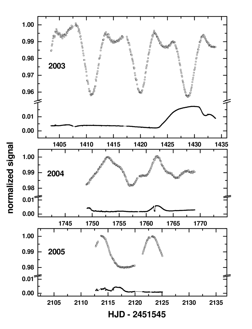
Figure 1.— MOST light curves for $\kappa^{1}$ Ceti from 2003, 2004, and 2005. The points are the mean signals from individual 101.413 min satellite orbits. The black connected symbols in the lower part of each panel are the the differences between the highest and lowest of 7 adjacent simultaneously recorded (background) Fabry images (see text). The ’dip’ at 1762 in 2004 corresponds to a total eclipse of the Moon.

Figure 2.— The marginalized likelihood for each of the fitted parameters is shown by the thick curve. The thin dotted curve shows the mean likelihood. The best-fitting value (the peak of the distribution) and the 68% credible regions determined from the marginalized likelihood are shown by the solid vertical, and dashed vertical lines. The unusual spike in the mean likelihood curve for a low value of k in the k histogram is likely due to low numbers of statistics, as indicated by the negligible value of the marginal likelihood curve.

Figure 3.— The solid lines are the 68% and 95% credible regions of the marginalized likelihood for various parameters. The 68% mean likelihood credible regions are shown by dotted contours (see text). Obviously there is little correlation between $k$ and $i$ in the bottom right panel.

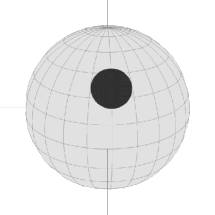
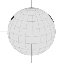
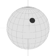
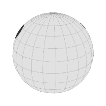
Figure 4.— The best-fitting two spot solution for $\kappa^{1}$ Ceti in 2003 (rotating counter-clockwise from top) and seen from the line of sight at phases 0.00, 0.25, 0.50, and 0.75 (from left) of the first spot. Middle: the MOST light curve with errors (see text). The continuous line is the solution from the “Minimum $\chi^{2}$” column of Table 3. The dotted line indicates the unspotted normalized signal of the star ($U$=1.0011). Vertical dashed lines indicate phases 0.00, 0.25, 0.50 and 0.75. Bottom: residuals from the model on the same scale.

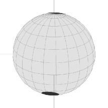
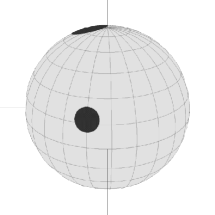
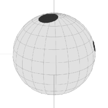
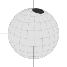
Figure 5.— The best-fitting three spot solution for $\kappa^{1}$ Ceti in 2004 (rotating counter-clockwise from top) and seen from the line of sight at phases 0.00, 0.25, 0.50, and 0.75 (from left) of the first spot. Middle: the MOST light curve with errors (see text). The continuous line is the solution from the “Minimum $\chi^{2}$” column of Table 3. The dotted line indicates the unspotted normalized signal of the star ($U$=1.0149). Vertical dashed lines indicate phases 0.00, 0.25, 0.50 and 0.75. Bottom: residuals from the model on the same scale.

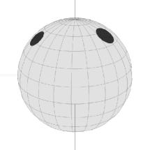
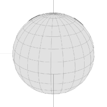
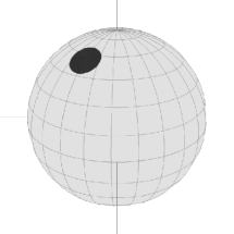
Figure 6.— The best-fitting two spot solution for $\kappa^{1}$ in Ceti 2005 (rotating counter-clockwise from top) and seen from the line of sight at phases 0.00, 0.25, 0.50, and 0.75 (from left) of the first spot. Middle: the MOST light curve with errors (see text). The continuous line is the solution from the “Minimum $\chi^{2}$” column of Table 3. The dotted line indicates the unspotted normalized signal of the star ($U$=1.0042). Vertical dashed lines indicate phases 0.00, 0.25, 0.50 and 0.75. Bottom: residuals from the model on the same scale.

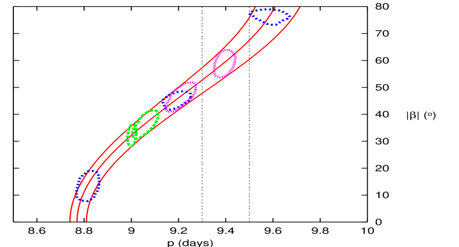
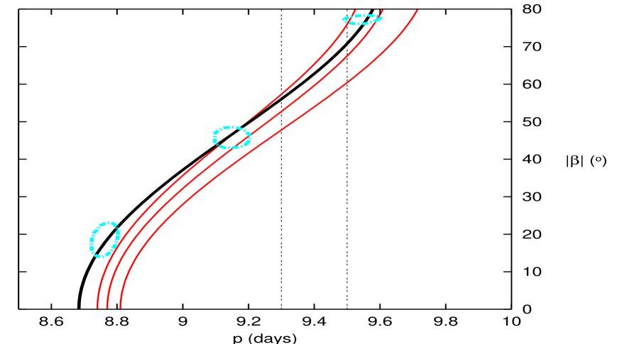
Figure 7.— Top: The 68 % marginalized likelihood contours for the modulus of the latitude, $|\beta|$, and spot period are shown by dots for each spot – 2003 (green), 2004 (blue) and 2005 (pink). The central red curve is the solar-period, latitude relation (Equation 1) with the mean values taken from Solution 1 of Table 3, $k$ = 0.090 and $P_{EQ}$ = 8.77$d$. The other two red lines correspond to $k$ = 0.085, $P_{EQ}$ = 8.74$d$, and $k$ = 0.096, $P_{EQ}$ = 8.81$d$. The vertical dashed lines indicate the range of rotational periods ($p$ = 9.4 $\pm$ 0.1 days) found in Ca II H & K line reversals over $\sim$30 years. Bottom: The 68 % marginalized likelihood contours for the 2004 data only (cyan) while fitting not for $k$ and $P_{EQ}$ but explicitly for the periods, $p_{2004\_1}$, $p_{2004\_2}$, and $p_{2004\_3}$. The black curve is the best-fitting curve ($k$ = 0.096 and $P_{EQ}$ = 8.68$d$) for the 2004 data, while the red curves are the same as in the upper panel. As can be seen, the black curve fits the data well and thus the observed differential rotation pattern is closely similar to solar.

References

- Baliunas et al. (1995) Baliunas, S.L., Donahue, R.A., Soon, W.H., Horne, J.H., Frazer, J., Woodard-Eklund, L., Bradford, M., Rao, L.M., Wilson, O.C., Zhang, Q., Bennett, W., Briggs, J., Carroll, S.M., Duncan, D.K., Figueroa, D., Lanning, H.H., Misch, T., Mueller, J., Noyes, R.W., Poppe, D., Porter, A.C., Robinson, C.R., Russell, J., Shelton, J.C., Soyumer, T., Vaughan, A.H., Whitney, J.H., 1995, ApJ, 438, 269
- Baliunas et al. (1983) Baliunas, S.L., Hartmann, L., Noyes, R.W., Vaughan, H., Preston, G.W., Frazer, J., Lanning, H., Middelkoop, F., Mihalas, S., 1983, ApJ, 275, 752
- Brown et al. (2004) Brown, B. P., Browning, M. K., Brun, A. S., Toomre, J. 2004, Proceedings of the SOHO 14 GONG 2004 Workshop (ESA SP-559). ”Helio- and Asteroseismology: Towards a Golden Future”. 12-16 July, 2004. New Haven, Connecticut, USA. Editor: D. Danesy., p.341
- Brun and Toomre (2002) Brun A.S., Toomre J. 2002, ApJ, 570, 865
- Budding (1977) Budding, E. 1977, Ap&SS, 48, 207
- Collier Cameron (2002) Collier Cameron, A. 2002, Astron. Nachr., 323, 336
- Croll (2006a) Croll, B. 2006, PASP, accepted 18 July
- Croll et al. (2006b) Croll, B., Walker, G. A. H., Kuschnig, R., Matthews, J.M., Rowe, J.F., Walker, A., Rucinski, S.M., Hatzes, A.P., Cochran, W.D., Robb, R.M., Guenther, D.B., Moffat, A.F.J., Sasselov, D., Weiss, W.W., 2006, ApJ, 648, 607
- Díaz-Cordovés et al. (1995) Díaz-Cordovés, J., Claret, A., Giminénez, A. 1995, Ap&SS, 110, 329
- Dorren (1987) Dorren, J.D. 1987, ApJ, 320, 756
- ESA (1997) European Space Agency. 1997. The Hipparcos and Tycho Catalogues (ESA SP-1200)(Noordwijk: ESA) (HIP)
- Gamerman et al. (1999) Gamerman D., 1997, Markov Chain Monte Carlo: Stochastic Simulation for Bayesian Inference, Chapman and Hall, London
- Gelman and Rubin (1992) Gelman, A., Rubin, D.B. 1992, Statistical Science, 7(4), 457
- Gilks et al. (1996) Gilks, W.R., Richardson, S., Spiegelhalter, D.J., 1996, Markov Chain Monte Carlo in Practice, Champan and Hall, London
- Gregory (2005a) Gregory, P.C. 2005a, ApJ, 631, 1198
- Gregory (2005b) Gregory, P.C. 2005b, Bayesian Logical Data Analysis for the Physical Sciences: A Comparative Approach with Mathematica Support (Cambridge: Cambridge Univ. Press)
- Güdel et al. (1997) Güdel, M., Guinan, E.F., & Skinner, S.L., 1997, ApJ, 483, 947
- Hall & Busby (1990) Hall, D.S. & Busby, M.R. 1990, in Active Close Binaries, NATO ASIC Proceedings 319, Nato Advance Study Institute, p. 377
- Henry et al. (1995) Henry, G.W., Eaton, J.A., Hamer, J. & Hall, D.S. 1995, ApJS, 97, 513
- Howard et al. (1983) Howard, R., Adkins, J.M., Boyden, J.E., Cragg, T.A., Gregory, T.S., Labonte, B.J., Padilla, S.P., Webster, L. 1983, Solar Phys. 83, 321
- Kitchatinov (2005) Kitchatinov, L.L. 2005, Physics - Uspekhi 48 (5), 449
- Lanza et al. (1998) Lanza, A. F., Catalano, S., Cutispoto, G., Pagano, I., Rodono, M., 1998, A&A, 332, 541
- Lebedinskii (1941) Lebedinskii, A.I. 1941, Astron. Zh., 18, 10
- Levenberg (1944) Levenberg, K., 1944, Quart. Appl. Math. 2, 164
- Lewis and Bridle (2002) Lewis, A., Bridle, S. 2002, PhRvD, 66, 103511
- Marquardt (1963) Marquardt, D.W., 1963, SIAM J. Appl. Math, 11, 431
- Messina & Guinan (2002) Messina, S. & Guinan, E. F. 2002, A&A, 393, 225
- Newton and Nunn (1951) Newton, H.W., Nunn, M.L. 1951, MNRAS, 111, 413
- Ossendrijver (2003) Ossendrijver, M. 2003, Astronomy and Astrophysics Review, Volume 11, Issue 4, 287
- Press et al. (1992) Press, W.H., Flannery, B., Teukolsky, S.A., Vetterling, W.T. 1992. Numerical Recipes in Fortran, 2nd ed. (Cambridge: Cambridge Univ. Press)
- Ribárik (2002) Ribárik, G., 2002, Occasional Technical Notes from Konkoly Observatory No. 12, http://www.konkoly.hu/Mitteilungen/otn12.ps.Z
- Ribárik et al. (2003) Ribárik, G., Oláh, K., Strassmeier, K. G. 2003, Astronomische Nachrichten, 324, 202
- Rucinski et al. (2004) Rucinski, S.M., Walker, G. A. H., Matthews, J.M., Kuschnig, R., Shkolnik, E., Marchenko, S., Bohlender, D.A., Guenther, D. B., Moffat, A. F. J., Sasselov, D., Weiss, W. W. 2004, PASP, 116, 1093
- Sajina et al. (2006) Sajina, A., Scott, D., Dennefeld, M., Dole, H., Lacy, M., Lagache, G., astro-ph 0603614
- Shkolnik et al. (2003) Shkolnik, E., Walker, G.A.H., Bohlender, D.A., 2003, ApJ, 597,1092
- Thompson et al. (2003) Thompson, M.J., Christensen-Dalsgaard, J., Miesch, M.S. 2003, Annu. Rev. Astron. Astrophys., 41, 599
- Walker et al. (2003a) Walker, G.A.H., Matthews, J.M., Kuschnig, R., Johnson, R., Rucinski, S., Pazder, J., Burley, G., Walker, A., Skaret, K., Zee, R., Grocott, S., Carroll, K., Sinclair, P., Sturgeon, D., Harron, J., 2003a, PASP, 115, 1023