Absolute Calibration and Characterization of the
Multiband Imaging Photometer for Spitzer. II. 70 micron Imaging

Karl D. Gordon¹¹affiliation: Steward Observatory, University of Arizona, Tucson, AZ 85721 , Charles W. Engelbracht¹¹affiliation: Steward Observatory, University of Arizona, Tucson, AZ 85721 , Dario Fadda²²affiliation: Spitzer Science Center, 220-6, Caltech, Pasadena, CA 91125 , John Stansberry¹¹affiliation: Steward Observatory, University of Arizona, Tucson, AZ 85721 , Stefanie Wachter²²affiliation: Spitzer Science Center, 220-6, Caltech, Pasadena, CA 91125 , Dave T. Frayer²²affiliation: Spitzer Science Center, 220-6, Caltech, Pasadena, CA 91125 , George Rieke¹¹affiliation: Steward Observatory, University of Arizona, Tucson, AZ 85721 , Alberto Noriega-Crespo²²affiliation: Spitzer Science Center, 220-6, Caltech, Pasadena, CA 91125 , William B. Latter³³affiliation: NASA Hershel Science Center, 100-22, Caltech, Pasadena, CA 91125 , Erick Young¹¹affiliation: Steward Observatory, University of Arizona, Tucson, AZ 85721 , Gerry Neugebauer¹¹affiliation: Steward Observatory, University of Arizona, Tucson, AZ 85721 , Zoltan Balog¹¹affiliation: Steward Observatory, University of Arizona, Tucson, AZ 85721 , Hervé Dole⁶⁶affiliation: Institut d’Astrophysique Spatiale (IAS), bât. 121, 91405 Orsay Cedex, France , Eiichi Egami¹¹affiliation: Steward Observatory, University of Arizona, Tucson, AZ 85721 , Dean Hines⁴⁴affiliation: Space Science Institute, 4750 Walnut Street, Boulder, CO 80301 , Doug Kelly¹¹affiliation: Steward Observatory, University of Arizona, Tucson, AZ 85721 , Francine Marleau²²affiliation: Spitzer Science Center, 220-6, Caltech, Pasadena, CA 91125 , Karl Misselt¹¹affiliation: Steward Observatory, University of Arizona, Tucson, AZ 85721 , Jane Morrison¹¹affiliation: Steward Observatory, University of Arizona, Tucson, AZ 85721 , Pablo Pérez-González¹¹affiliation: Steward Observatory, University of Arizona, Tucson, AZ 85721 ⁵⁵affiliation: Departamento de Astrofísica, Facultad de CC. Físicas, Universidad Complutense de Madrid, E-28040 Madrid, Spain , Jeonghee Rho²²affiliation: Spitzer Science Center, 220-6, Caltech, Pasadena, CA 91125 , and Wm. A. Wheaton²²affiliation: Spitzer Science Center, 220-6, Caltech, Pasadena, CA 91125

Abstract

The absolute calibration and characterization of the Multiband Imaging Photometer for Spitzer (MIPS) 70 µm coarse- and fine-scale imaging modes are presented based on over 2.5 years of observations. Accurate photometry (especially for faint sources) requires two simple processing steps beyond the standard data reduction to remove long-term detector transients. Point spread function (PSF) fitting photometry is found to give more accurate flux densities than aperture photometry. Based on the PSF fitting photometry, the calibration factor shows no strong trend with flux density, background, spectral type, exposure time, or time since anneals. The coarse-scale calibration sample includes observations of stars with flux densities from 22 mJy to 17 Jy, on backgrounds from 4 to 26 MJy sr^-1, and with spectral types from B to M. The coarse-scale calibration is $702\pm 35$ MJy sr^-1 MIPS70^-1 (5% uncertainty) and is based on measurements of 66 stars. The instrumental units of the MIPS 70 µm coarse- and fine-scale imaging modes are called MIPS70 and MIPS70F, respectively. The photometric repeatability is calculated to be 4.5% from two stars measured during every MIPS campaign and includes variations on all time scales probed. The preliminary fine-scale calibration factor is $2894\pm 294$ MJy sr^-1 MIPS70F^-1 (10% uncertainty) based on 10 stars. The uncertainty in the coarse- and fine-scale calibration factors are dominated by the 4.5% photometric repeatability and the small sample size, respectively. The 5 $\sigma$ , 500 s sensitivity of the coarse-scale observations is 6–8 mJy. This work shows that the MIPS 70 µm array produces accurate, well calibrated photometry and validates the MIPS 70 µm operating strategy, especially the use of frequent stimulator flashes to track the changing responsivities of the Ge:Ga detectors.

Subject headings:

instrumentation: detectors

^†^†slugcomment: PASP, in press

1. Introduction

The Multiband Imaging Photometer for Spitzer (MIPS, Rieke et al., 2004) is the far-infrared imager on the Spitzer Space Telescope (Spitzer, Werner et al., 2004). MIPS images the sky in bands at 24, 70, and 160 µm. The absolute calibration of the MIPS bands is complicated by the challenging nature of removing the instrumental signatures of the MIPS detectors as well as predicting the flux densities of calibration sources accurately at far-infrared wavelengths. This paper describes the calibration and characterization of the 70 µm band. Companion papers provide the transfer of previous absolute calibrations to the MIPS 24 µm band (Rieke et al., 2007), the 24 µm band calibration and characterization (Engelbracht et al., 2007), and 160 µm band calibration and characterization (Stansberry et al., 2007). Engelbracht et al. (2007) also presents the MIPS stellar calibrator sample that is used for this paper. The calibration factors derived in these papers represent the official MIPS calibration and are due to the combined efforts of the MIPS Instrument Team (at Univ. of Arizona) and the MIPS Instrument Support Team (at the Spitzer Science Center).

The characterization and calibration of the MIPS 70 µm band is based on stellar photospheres. The repeatability of 70 µm photometry is measured from observations of two stars, at least one of which is observed in every MIPS campaign. The absolute calibration of the 70 µm band is based on a large network of stars observed in the standard coarse-scale photometry mode with a range of predicted flux densities and backgrounds. In addition to the coarse-scale observations, a small number of stars were observed in the fine-scale photometry mode to allow the coarse-scale calibration to be transfered to this mode. The observations used in this paper include both In Orbit Checkout (IOC, MIPS campaigns R, V, X1, and W) and regular science operations (MIPS campaigns 1-29) with a cutoff date of 3 Mar 2006.

The goal of the calibration is to transform measurements in instrumental units to instrument independent physical units. The goal of the characterization is to determine if the calibration depends on how the data are taken (e.g., exposure time, time since anneal) or characteristics of the sources being measured (e.g., flux density, background). The primary challenge for the 70 µm characterization and calibration is accurately correcting the detector transients associated with Ge:Ga detectors. The standard reduction steps are detailed in Gordon et al. (2005) but extra steps to achieve accurate photometry with the highest possible signal-to-noise for point sources are needed and discussed in this paper.

Accurate calibration and high sensitivity is important at 70 µm as they enable a number of science investigations including the detection and study of cold disks around stars (e.g., Kim et al., 2005; Bryden et al., 2006), imaging of warm dust in galaxies (e.g., Calzetti et al., 2005; Dale et al., 2005; Gordon et al., 2006), and investigation of faint, redshifted galaxies (e.g., Dole et al., 2004a; Frayer et al., 2006a).

2. Data

The 70 µm calibration program is based on stars with spectral types from B to M, predicted flux densities from 22 mJy to 17 Jy, and predicted backgrounds from 4 to 26 MJy/sr (Engelbracht et al., 2007). The observations were carried out in photometry mode with 3.15 to 10.49 s individual image exposure times and a range of total exposure times from $\sim$ 50 s to $\sim$ 560 s. The majority of the observations were performed in standard coarse-scale photometry mode with a few done in the standard fine-scale photometry mode. The coarse- and fine-scale photometry modes are also referred to as the wide- and narrow-field photometry modes.

The coarse-scale mode samples the 18″ FWHM 70 µm PSF with 9.85″ pixels. The minimum coarse-scale photometry mode observation consists of 12 images of the target and 4 images where the internal calibration stimulator is flashed (see Fig. 2 of Gordon et al., 2005). The target point source is dithered around the central part of good half of the 70 µm array so that the source is on different pixels for each of the 12 image exposures. The stimulator flashes are used to remove the responsivity variations in the Ge:Ga detectors by dividing each image exposure by an interpolated stimulator flash. This division converts the raw DN/s units to fractions of the stimulator flash amplitude (also measured in DN/s units) which are termed MIPS70 units. These MIPS70 units are surface brightness units as the varying pixel size across the array has been normalized out due to the division by the stimulator flash. Readers should refer to Rieke et al. (2004) and Gordon et al. (2005) for the details on how MIPS data are taken and reduced. The maximum image exposure time is 10.49 s, thus longer total exposures on a source are acquired by repeating the minimum set of images described above.

The fine-scale mode samples the same 70 µm PSF with 5.24 ″ pixels and is designed for detailed studies of source structure. The dithering strategy is different for fine-scale mode where source-background pairs of images are acquired instead of dithering the source around the array. The minimum fine-scale photometry mode observation consists of 8 source-background pairs of images, 4 stimulator images, and 2 dedicated stimulator background images. The data reduction is the same as the coarse-scale mode and, thus, the resulting raw units of the images are also fractions of the stimulator flash and are termed MIPS70F units. These units are different than the MIPS70 units due to the change in the optical train used.

The coarse-scale observations were extensive and motivated to check non-linearities versus flux density, background, exposure time, etc. The fine-scale observations were done to transfer the coarse-scale calibration to the fine-scale. The coarse-scale and scan map modes share the same optical train and only differ in the dithering strategy, thus the coarse-scale photometry calibration should apply to the scan map mode observations.

2.1. Data Reduction

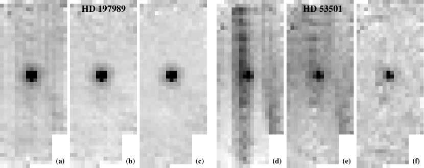
Refer to caption — Figure 1.— The mosaics of coarse-scale observations of two stars of different brightness are shown with (a,d) default reductions, (b,e) column mean subtraction, and (c,f) column mean subtraction and time filtering. The two stars are HD 197989 (AOR #13590784, flux density = 787 mJy) and HD 53501 (AOR #13641984, flux density = 135 mJy). The HD 197989 images are displayed with a linear stretch that ranges from 0.022 to 0.05 (a), -0.005 to 0.025 (b), and -0.005 to 0.0025 (c). The HD 53501 images are displayed with a linear stretch that ranges from 0.009 to 0.025 (d), -0.005 to 0.01 (e), and -0.002 to 0.008 (f). The images and ranges are all given in MIPS70 units.

Each observation was reduced through the MIPS Data Analysis Tool (DAT, v3.06, Gordon et al., 2005). The resulting mosaics of this default processing are shown in Fig. 1a,d for two point sources observed in coarse-scale mode. It is possible to improve the detection of point sources taken in photometry mode by utilizing the redundancy of the observations to remove residual instrumental signatures. These residual signatures arise because the stimulator flashes calibrate the fast response of the detectors well, but there is a drift between the fast and slow response of the detectors (Haegel et al., 2001; Gordon et al., 2005). In coarse-scale mode, point sources are dithered around the array to ensure their signals are in the well calibrated fast response. The dithering does not put the background signal in the fast response and as the sky level is roughly equal at the different dither positions, the background is in the slow response regime. As an accurate measurement of the background is essential for good photometry, the drifting background needs to be corrected by two additional steps. The extra steps are designed not to introduce biases into the data based on source flux density while reducing the residual instrumental signatures.

The largest portion of the drift is seen to be in common among pixels in the same column. This is not surprising as columns represent a common strip of detector material (Young et al., 1998). The column offset can be removed easily for observations of isolated point sources by subtracting the median of the column. The median of each column is computed after excluding a region centered on the source with a diameter of 9 pixels ( $\sim$ 89″) to ensure the resulting correction is not biased by the source. The column subtracted data are shown in Fig. 1b,e. A smaller, but still significant background drift seen as array dependent structure is still present after this correction. This smaller residual instrument signature can be removed from each pixel by using a simple time filter. This time filter works by subtracting the mean value from a pixel of the previous and next 14 measurements of that pixel. To ensure that this mean value is not biased by the presence of the source itself, all measurements of the source within a spatial radius of 4.5 pixels as well the current, previous, and next measurements are not used in computing the mean value. The mean is computed after excluding all the pixels $>4\sigma$ from the median (sigma clipping). The time filter only uses data taken on a particular source which means that the time filtering is less accurate at the beginning and end of the observation set. This time filtering with constraints was optimized to minimize the background noise. The result is shown in Fig. 1c,f. From the two examples shown in Fig. 1, it is clear that the importance of these extra processing steps increases with decreasing source flux density.

Unlike coarse-scale photometry mode where the large field of view provides sufficient area for background estimates, the reduced field of view of the find-scale mode requires that the point source be chopped off the array. This simplifies the extra processing to just subtracting the images taken in the off positions from the on position images which effectively removes the column offsets and smaller scale pixel dependent drifts in the background.

2.2. Aperture Corrections

A necessary part of measuring the flux density of a point source using aperture photometry or point spread function (PSF) fitting is an accurate PSF. The repeatability measurements on HD 163588 and HD 180711 provide the ideal opportunity to compare the STinyTim (Krist, 2002) model of the MIPS 70 µm PSF to the coarse-scale observations. The repeated observations of these two stars allow for very high signal-to-noise observed PSFs to be constructed. All of the observations of these two stars taken after the final optimization of the array parameters ( $\geq$ 5th MIPS campaign) were mosaiced to produce two empirical PSFs. The fine-scale observed PSFs are from observations of the fine-scale calibration stars. The observed PSFs are compared with the STinyTim PSF for a T = 10000 K blackbody in Fig. 2. All stars in our calibration program have the same spectrum across the 70 µm band as the Rayleigh-Jeans tail of stellar spectra is being sampled. Thus, the PSF generated assuming a T = 10000 K blackbody is a good representation of any star’s PSF as long as it does not have an infrared excess.

As can be seen for both coarse- and fine-scale, the model PSF well represents the observed PSFs when the smoothing associated with the pixel sampling is applied. We have simulated the pixel sampling smoothing two different methods. The first method used uses the mips_simulator program which produces simulated MIPS observations with the observed dithering using an input PSF. These simulated observations where mosaiced, using the same software which is used for the actual observations, to produce the mips_simulator PSF shown. The second method uses a simple boxcar smoothing function. The “smooth=1.35 pix” and “smooth=1.5 pix” PSFs are created by directly smoothing the STinyTim PSF with a square kernel with the specified width where the pixel sizes are 9.85 $\arcsec$ and 5.24 $\arcsec$ for the coarse- and fine-scales, respectively. The close correspondence between the observed, mips_simulator, and directly smoothed PSFs means that accurate MIPS 70 µm PSFs can be generated from the STinyTim PSF smoothed with a simple square kernel.

The correspondence between the observed and STinyTim model PSFs was expected as the MIPS 70 µm band should be purely diffraction limited. The 70 µm band has a bandwidth of $\sim$ 19 µm resulting in the PSF varying significantly between blue (peaking at wavelengths shorter than the band) and red (peaking at wavelengths longer than the band) sources. In addition to stellar sources, we have verified that STinyTim model PSFs describe the observed PSFs for sources with blackbody temperatures as low as 60 K using observations of asteroids and Pluto. Having a valid model for the PSF allows for accurate, noiseless aperture corrections as the total flux density is known from PSFs created with different source spectra.

The observed fine-scale PSFs do show disagreement in the core, where the model PSF is systematically higher. This is not surprising given that there are known flux density nonlinearities in the Ge:Ga detectors that are not corrected in the standard data reduction and the fine-scale calibration stars are brighter than those observed in the coarse-scale mode. Characterization of these flux density nonlinearities is ongoing, but preliminary indications are that they are $\sim$ 15% for point source flux densities of $\sim$ 20 Jy observed in the coarse-scale mode (see §3.1). The coarse-scale observed PSFs do not show any systematic disagreement in the core, consistent with the use of fainter stars.

The aperture corrections were calculated by performing aperture photometry on square kernel smoothed model PSFs. The model PSFs were computed for a $64\arcmin\times 64\arcmin$ field to ensure that the total flux of a point source was measured. The method for computing the aperture corrections is the same as used for measuring the calibration star flux densities used in this paper. The method does not account for partial pixels but given that the model PSFs were computed with pixels 10 $\times$ smaller than the array pixel size this is not expected to be an issue even for the smallest apertures considered in this paper. For the purposes of this paper, we use the radius = 35″ aperture (1.22 aperture correction) to minimize the sensitivity of the calibration to uncertainty in the aperture correction and centering errors. The aperture corrections for a small sample of object aperture and background annuli are given in Table 1 for three PSFs (T = 10000 K, 60 K, and 10 K blackbodies). Three PSFs with different source spectra are given to emphasize the importance of using PSFs with the right source spectrum for accurate photometry.

2.3. Measurements

The photometry was measured with aperture photometry and PSF fitting for each observation of a calibration star. The aperture photometry was done with a circular aperture with a radius of $35\arcsec$ and a sky annulus of 39 to $65\arcsec$ . The PSF fitting was done with StarFinder (Diolaiti et al., 2000) which is ideally suited for the well sampled and stable MIPS PSFs. The flux densities measured with these two methods are listed in Tables 2-3. The aperture flux densities have had the aperture correction applied and the PSF flux densities are naturally for an infinite aperture. In addition to the reported flux densities, signal-to-noise (S/N) calculations are also reported. In the case of the aperture photometry, the S/N calculation is done using the noise in the sky annulus to determine both the uncertainty due to summing the object flux density as well as subtracting the background. This S/N does not include the contribution from the photon noise of the source as the gain of Ge:Ga detectors is not a well defined quantity. In the case of the PSF photometry, the S/N calculation is done by the StarFinder program utilizing the empirical uncertainty image calculated from the repeated measurements of each point in the mosaic. Only measurements with S/N greater than 5 are reported in Tables 2-3. The columns in these tables give the star name, campaign of observation, AOR # (unique Spitzer observation identifier), exposure start time, individual exposure time, total exposure time, aperture flux density, signal-to-noise, PSF flux density, and signal-to-noise.

The measurements used in this paper were all reduced with the DAT and custom software based on the DAT results. Comparisons were done with measurements using data reduced with the Spitzer Science Center (SSC) pipeline and similar software available from the contributed software portion of the Spitzer website¹¹1http://ssc.spitzer.caltech.edu/archanaly/contributed/. Note that the SSC pipeline reduced images are given in MJy sr^-1 and must be divided by the applied flux conversion factor (given by the FITS header keyword FLUXCONV) to recover the instrumental MIPS70 or MIPS70F units. The result of this comparison is that the two methods produce equivalent results with a mean ratio of DAT to SSC aperture photometry for the full sample of $0.994\pm 0.037$ .

2.4. Flux Density Predictions

The predicted flux densities at 70 µm were derived from the 24 µm predictions presented by Engelbracht et al. (2007) using 24/70 µm colors derived from models. For each star, the ratio of the flux densities at the effective filter wavelengths of 23.675 µm and 71.42 µm was computed for the appropriate Kurucz (1993) model (using a power-law interpolation) and a blackbody at the effective temperature of the star. The model ratio was taken to be the average of these two values, which typically differed by 1-2%, and the uncertainty was taken to be the difference between them. The predicted flux densities at 24 µm were divided by this ratio to compute the 70 µm flux densities. The uncertainties on the flux density predictions were calculated by adding in quadrature the uncertainties in the 24 µm flux density and in the 24/70 µm color prediction. The average predicted backgrounds for the observations were estimated from Spitzer Planning Observations Tool (SPOT) with the uncertainties giving the range when each target is visible. The full sample of calibration stars covers a wide range of ecliptic and Galactic latitudes providing a large range in backgrounds, but for any particular star the backgrounds vary by $<$ 30% for different dates of observation. The flux density predictions and background estimates are listed in Tables 4 & 5. These tables also give each star’s spectral type, the average of the measured aperture and PSF flux densities and their associated signal-to-noises. In addition, the average calibration factor determined using the aperture and PSF fitting measurements is given (see §3.1).

The zero point of the 70 µm band at the effective filter wavelength of 71.42 µm is $0.778\pm 0.012$ Jy in the Rieke et al. (2007) system. It is important to note that the 70 µm calibration is based on stars (10,000 K blackbody). Thus, measuring accurate 70 µm flux densities for objects with different spectral energy distributions requires the use of the color corrections given in Stansberry et al. (2007).

3. Results

The first step in deriving the final calibration factor is to examine the ensemble of calibration factor measurements for stars which show significant deviations. These deviations can be the result of a star having an infrared excess, a poor flux density prediction, or a measurement corrupted by extended emission. Infrared excesses and poor flux density predictions can be seen by calculating the calibration factor for each star and identifying stars that give calibration factors that are significantly deviant from the ensemble. Stars with excesses will have measured flux densities well in excess of the predicted flux densities and, thus, will predict low calibration factors compared to non-excess stars. Figure 3 displays the calibration factors for all the calibration stars versus predicted flux density. The calibration factors are calculated as a conversion from MIPS70 units to MJy sr^-1 as the basic measurement made by the 70 µm detectors is flux per pixel which is a surface brightness (see §3.6 for the conversion from MIPS70 units directly to flux densities assuming the default 70 µm mosaic pixel size). Measurements using both aperture photometry and PSF fitting are shown in this figure. The PSF fitting values show less scatter than the aperture photometry values and, thus, will be the basis for identifying deviant measurements. We identify two stars (HD 102647 and HD 173398) which have possible excesses from Fig. 3 and no stars with poor flux density predictions. There are seven stars that have significant extended emission underlying or near the object position determined by visual inspection of the 70 µm images. During this inspection, it was seen that the observation of HD 173511 was affected by a nearby, much brighter object and, as a result, this star was also rejected. The stars in our sample that have been rejected for any of these three reasons are listed in Table 6. If a star was rejected as part of the 24 µm analysis given in Engelbracht et al. (2007), it is not used at all in this paper.

3.1. Flux Density/Background Nonlinearities

A possible source of scatter in the calibration factor measurements is flux density nonlinearities that are a characteristic of Ge:Ga detectors. In contrast to electronic nonlinearities that depend solely on total flux density, flux density nonlinearities are due to the change in rate of flux density falling on the detectors (e.g., when a source chops onto a detector). Given that the nonlinearity is due to a change in flux density on the detector, the flux density nonlinearity could depend on background as well as source flux density. The electronic nonlinearities are small ( $\sim 2$ %) for the MIPS 70 µm pixels and are corrected when the data are reduced (Gordon et al., 2005). Fig. 4 shows the calibration factors versus predicted flux densities and backgrounds. The calibration factors have been calculated from the average of all the measurements of each star and the uncertainty on the average includes the flux density prediction uncertainty. The calculated calibration factors for each star are listed in Tables 4 & 5.

It is clear that flux density nonlinearities are present in the aperture photometry data but are much smaller or non-existent in the PSF fitting photometry. A direct comparison of the aperture and PSF fitting measurements is shown in Fig. 5. Starting at around $\sim$ 1 Jy, the aperture measurements begin to underestimate the PSF measurements while below $\sim$ 200 mJy, the aperture to PSF fitting ratio shows a large scatter. For bright sources, the flux density nonlinearities will show up at the peak of the PSF and the PSF fitting compensates as relatively more weight is given to the wings of the PSF than in aperture photometry. For faint sources, the PSF fitting shows less scatter since it more accurately accounts for nearby faint sources and background structure than aperture photometry. For these reasons, we will use the PSF fitting measurements for the rest of this work.

The PSF fitting measurements show that the 70 µm calibration measurements are linear between 22 mJy and 17 Jy. A linear fit to these data (accounting for the uncertainties in both x and y values) gives

{\rm Factor}=(693\pm 18)+(2.9\pm 5.8)\log(F(\nu))

(1)

where $F(\nu)$ is the flux density in mJy. There are four stars (HD 31398, 120933, 213310, & 216131) that are $>5\sigma$ from the mean calibration factor and are identified with square boxes in Fig. 4. The large deviations of these four stars are most likely due to weak infrared excesses as the derived calibration factor is low compared to the ensemble. These four stars have been excluded from the fit and from the rest of the paper. The slope value is consistent with no nonlinearities; the upper limit on the nonlinearities is computed to be 1.5% from the ratio of the fit values at 10 mJy and 20 Jy . The fit to the aperture photometry shows a 42% nonlinearity between the same limits.

A similar result is found for the calibration factor versus background. The linear fit to the PSF fitting results gives a slope of $91\pm 20$ , which is consistent with no slope at the $5\sigma$ level. There is a statistically significant slope for the linear fit for the aperture photometry results, but this may just be an artifact of the nonlinearity seen versus flux density. A comparison of the two left hand plots in Fig. 4 shows that the correlation is better versus flux density than versus background.

3.2. Repeatability

The photometric repeatability and trends in time can be measured from the two stars that have been observed throughout MIPS operations. The photometric repeatability is how well the raw flux of a star can be measured and is determined from multiple observations of the same star. Each measured flux density from PSF fitting photometry was normalized to the average flux density of each star and plotted in Fig. 6. The sigma clipped average in 15 bins between 50 and 950 days since launch is also plotted. The dotted vertical lines identify changes in the default dither pattern, bias voltage, and instrument software. This plot clearly shows that the 70 µm array displays measurable long term variations. The measurements show that the response dropped from the starting value by $\sim$ 7% around day 200 then recovered to slightly above the starting value around day 300. After this, the response seems to have stabilized with evidence for a weak trend downward. While it is tempting to identify the initial variations with the changes in how the data were taken, no clear instrumental parameter has been identified that would cause these variations. Initial testing with other methods of measuring the brightness of these two stars has shown similar, but not identical variations. More work is clearly needed to understand the origin of the initial variations.

Even given the initial variations, the repeatability of the two stars is quite good. The repeatabilities for all the measurements are 4.5% for HD 163588 and 3.7% for HD 180711. For reference, the repeatabilities for aperture photometry using the same data are 4.9% for HD 163588 and 3.9% for HD 180711. Given the changes in the operating parameters of the 70 µm array early in the mission, we also computed the repeatabilities using only the data taken after the last change. The repeatabilities for all the measurements after the 8th MIPS campaign are 2.9% for HD 163588 and 2.7% for HD 180711. For reference, the repeatabilities for aperture photometry using the same data are 4.3% for HD 163588 and 3.4% for HD 180711. The combined measurements imply a conservative repeatability of the MIPS 70 µm array of $\sim$ 4.5%.

3.3. Time Since Anneal

The MIPS 70 µm array is annealed by raising the temperature by a few degrees to remove cosmic ray damage. This was done every six hours till MIPS campaign 20 and every three to four hours since then. Residual instrumental signatures are seen to grow with time since anneal and this change was made to minimize them. In addition to removing cosmic ray damage, the responsivity of the array is reset (Rieke et al., 2004). The calibration factor should not have a dependence on time since anneal as all 70 µm measurements are referenced to the internal simulator measurements taken every two minutes or less. To check this, Figure 7 shows the calibration factor versus anneal time. No trend is seen.

3.4. Other Checks

The accuracy of the flux density predictions can be checked by comparing the calibration factor derived for stars of different spectral types. The stars in the sample can be divided into three categories; hot stars (B & A dwarfs), solar analogs (early G dwarfs), and cool stars (K & M giants). The weighted average calibration factors (after sigma clipping) for these three categories are $717\pm 8$ , $717\pm 3$ , and $701\pm 6$ MJy sr^-1 MIPS70^-1 where the number of measurements contributing to each class are 11, 6, and 58, respectively. None of averages are significantly different from each other, especially when the small number of measurements contributing to the hot stars and solar analogs are taken into account.

The dependence on exposure time was checked by computing the weighted average calibration factor separately for observations taken with 3.15 and 10.49 s. The resulting calibration factors are $701\pm 6$ and $723\pm 7$ MJy sr^-1 MIPS70^-1 with 62 and 12 measurements contributing to the averages, respectively. As the difference is only $2.4\sigma$ , no significant systematic change with exposure time is seen.

3.5. Noise Characteristics

The behavior of the noise is plotted versus predicted flux density in Fig. 8 for the PSF fitting measurements. To compare measurements taken at different exposure times, each noise measurement has been transformed to the equivalent noise in 500 s assuming a $t^{0.5}$ dependence. The noise behavior can be characterized by

\sigma(\mathrm{500s})^{2}=0.90^{2}+[0.20\mathrm{F(\nu)}^{0.5}]^{2}+[0.0022\mathrm{F(\nu)}]^{2}

(2)

where $F(\nu)$ is the predicted 70 µm flux density in mJy. The first term accounts for the confusion noise, the second term the photon noise, and the third term the noise due to the division by the interpolated stimulator flash.

The sensitivity of the MIPS 70 µm band in 500 s can be determined from this fit by computing where the flux is 5 $\times$ the uncertainty from Eq. (2). The 5 $\sigma$ , 500 s sensitivity computed in this fashion is $\sim$ 5 mJy. This measurement is based on an extrapolation of over a factor of ten from the lowest measured point and so is fairly uncertain. The sensitivity can be better measured from deep cosmological surveys. The Extragalactic First Look Survey gives a 5 $\sigma$ , 500 s sensitivity of $\sim$ 6 mJy after correcting for the updated calibration factor (Frayer et al., 2006a). Somewhat worse sensitivities up to $\sim$ 8 mJy are seen for other deep MIPS 70 µm cosmological fields (D. Frayer, C. Papovich, private communication). This sensitivity can include a contribution from confusion, but this is likely to be small since the 5 $\sigma$ confusion noise for MIPS 70 µm coarse-scale observations is estimated at $\sim$ 1.5–3 mJy (Dole et al., 2004b; Frayer et al., 2006b). Combining the results from the calibration stars and deep cosmological field gives a conservative 5 $\sigma$ , 500 s sensitivity of 6–8 mJy.

3.6. Coarse-Scale Calibration

The final coarse-scale calibration is based on the PSF fitting results from all the observations (top, right plot in Fig. 4). The final calibration factor of $702\pm 35$ MJy sr^-1 MIPS70^-1 was determined by performing a weighted average of the calibration factors measured for each star. There are 66 calibration stars that contribute to this calibration factor. The calibration accuracy is dominated by the 4.5% repeatability uncertainty, but also includes contributions from the uncertainty of the mean (very small) and the 2% systematic uncertainty in the 24/70 µm flux density ratios. The conversion directly to flux densities from MIPS70 units implied by the measured calibration factor is $1.60\pm 0.08$ Jy MIPS70^-1 given the instrumental flux densities were measured on mosaics with $9.85\arcsec\times 9.85\arcsec$ pixels. The calibration factor determined from the 57 stars taken after the 9th MIPS campaign is $696\pm 34$ MJy sr^-1 MIPS70^-1. This shows that the calibration factor is not significantly changed by the variations in the repeatability stars seen prior to the 9th MIPS campaign. The calibration factor determined from the aperture measurements is $704\pm 35$ MJy sr^-1 MIPS70^-1 where only measurements from 0.3 to 1 Jy are used (see Figs. 4 & 5). This shows that the calibration derived from aperture and PSF fitting measurements are equivalent in the restricted range where the aperture photometry produces accurate results.

The preliminary calibration factor determined soon after launch was $634\pm 127$ MJy sr^-1 MIPS70^-1. The new value is 11% larger than this preliminary value, well within the 20% uncertainty in the preliminary value. This 11% change is not unexpected given that the preliminary value was based on a handful of measurements of a single star and the data reduction at the time did not include the extra steps to correct residual instrumental signatures. Existing data can be corrected to the new calibration factor by multiplying by the ratio of the new to old calibration factors. Note the calibration factor applied to data reduced using the SSC pipeline is given by the FITS header keyword FLUXCONV.

The coarse-scale calibration factor is determined from photometry mode observations, but should apply directly to scan map mode observations as both modes share the same optical train and only differ in the dithering strategy. The relative response between the scan map and coarse-scale photometry mode has been checked by observing the same source in both modes. It was found that the same flux density was measured within the uncertainties.

The consistency of the 70 µm calibration with the 24 µm calibration was checked using stars that were observed at both 24 and 70 µm. There are 36 such measurements for stars with 24 µm flux densities below 4 Jy (24 µm saturation limit). The resulting sigma clipped average of the ratio of the observed to model 24/70 color ratio is $1.002\pm 0.013$ showing that the 24 and 70 µm calibrations are consistent.

3.7. Extended Versus Point Source Calibration Check

The calibration factor determined above was calculated from observations and predictions of point sources. Given the complex response of Ge:Ga detectors to sources with different spatial extents, it is important to verify that the point source calibration applies to extended sources. This can be checked by comparing the total fluxes of resolved galaxies measured at 70 µm to those predicted by Infrared Astronomical Satellite (IRAS, Beichman et al., 1988) measurements at 60 and 100 µm. Galaxies provide good objects for such a check as they are discrete extended sources that were well measured by IRAS and have a significant component of their flux that is resolved by MIPS at 70 µm.

The comparison is done using the 75 Spitzer Infrared Nearby Galaxies Survey (SINGS, Kennicutt et al., 2003) galaxies from global measurements given by Dale et al. (2005) and updated by Dale et al. (2007). This sample is supplemented at the highest flux densities with global measurements of M31 (Gordon et al., 2006), M33 (Hinz et al., 2004), M101 (Gordon et al. in prep.), and the Large Magellanic Cloud (LMC, Meixner et al., 2006). The predictions of the 70 µm flux densities from the IRAS 60 and 100 µm measurements were done by first color correcting the IRAS measurements using the measured 60/100 flux density ratio to pick the appropriate power law color correction (Beichman et al., 1988) and then interpolating to the effective wavelength of the MIPS 70 µm band of 71.42 µm. The average color corrections were 1.0 for both IRAS 60 and 100 bands. The MIPS 70 µm measurements were corrected to the updated calibration factor and color corrected using the correction for the same power law determined for the IRAS measurements (Stansberry et al., 2007). The average MIPS 70 µm color correction was 0.93. Figure 9 gives the ratio of the MIPS to predicted IRAS 70 µm flux densities for all the galaxies with flux densities above 1 Jy. The weighted average of this ratio is 0.99 which is well within the uncertainties on the absolute calibration of MIPS 70 µm (5%) and IRAS 60 µm (5%, Beichman et al., 1988). This shows that the the MIPS 70 µm point source calibration applies for extended sources. This comparison also serves as another check that the photometry and scan observing modes share the same calibration even through the calibration factor is derived from photometry mode observations while the galaxies were observed with the scan map mode.

3.8. Fine-Scale Calibration

The fine-scale calibration should be similar to the coarse-scale calibration modulo the different pixel scales (5.24 instead of 9.85″ pixel^-1) and optical trains. Fig. 10 shows the calibration factor for PSF fitting photometry. The fine-scale calibration factor determined from these data is $2894\pm 294$ MJy sr^-1 MIPS70F^-1. The conversion directly to flux densities from MIPS70F units implied by this calibration factor is $1.87\pm 0.188$ Jy MIPS70^-1 given the instrumental flux densities were measured on mosaics with $5.24\arcsec\times 5.24\arcsec$ pixels. The fine-scale calibration factor is 4.12 $\times$ the coarse-scale factor. This is larger than the ratio of pixel areas (3.53) implying that the different optical train has a significant effect on the calibration. Only 10 calibration stars are used for the fine-scale calibration and, as a result, the fine-scale calibration must be taken as preliminary. The uncertainty on the fine-scale calibration is formally only 5%, but we have doubled this to account for the small sample used. In general, the fine-scale mode should be used for probing structure and the coarse-scale used when accurate photometry is needed.

3.9. Comparison to Previous Missions

The repeatability, absolute calibration accuracy, and sensitivity of the coarse-scale MIPS 70 µm band can be compared to previous missions. Imaging of point sources in bands similar to the MIPS 70 µm band has been provided in the past by the IRAS and the Infrared Space Observatory (ISO, Kessler et al., 1996).

IRAS 60 µm photometry of points sources has a repeatability of 11% and an absolute calibration uncertainty of 5% (Beichman et al., 1988). The IRAS Faint Source Catalog (Moshir et al., 1992) is 94% complete at 0.2 Jy. The almost full sky coverage of IRAS allows for a comparison of the IRAS 60 µm and MIPS 70 µm fluxes. There are 30 stars with both MIPS 70 µm and IRAS 60 µm Faint Source Catalog measurements (Moshir & et al., 1990) and IRAS 60 µm fluxes above 0.6 Jy. The average ratio of the IRAS 60 µm to MIPS 70 µm flux densities is $1.35\pm 0.01$ and the expected ratio from a Rayleigh-Jeans model is 1.42. Thus, the IRAS 60 µm flux densities need to be multiplied by 1.05 in order to put them on the Rieke et al. (2007) system.

The (ISOPHOT, Laureijs et al., 2003) instrument included a 70 µm band with the P3 detector and a 60 µm band with the C100 detector. The P3 reproducibility was 10-20% and absolute accuracy was 7%. The C100 repeatability was 3-20% and absolute accuracy was 15-25% (Klaas et al., 2003). The sensitivity of ISOPHOT in these bands is approximately 7.5-20 mJy $1\sigma$ in 256 s (Laureijs et al., 2003) which corresponded to a 5 $\sigma$ , 500 s sensitivity of 30-70 mJy. This sensitivity is better than that found from the 95 µm deep field observations of Rodighiero et al. (2003) where the 3 $\sigma$ , 5184 s sensitivity is 16 mJy which corresponds to a 5 $\sigma$ , 500 s sensitivity of 86 mJy.

The MIPS 70 µm observations compare favorably, with better repeatability (4.5%), as good or better absolute calibration uncertainty (5%), and higher sensitivity (6-8 mJy 5 $\sigma$ , 500 s) than previous missions imaging in similar bands. This is to be expected as the MIPS 70 µm detector operation has benefited from lessons learned from past missions.

4. Summary

The calibration of the MIPS 70 µm coarse- and fine-scale imaging modes was determined from many observations taken over the first 2.5 years of the Spitzer mission.

1.

The characterization and calibration of the MIPS 70 µm coarse-scale mode was determined from measurements of 78 stars with spectral types from B to M, with flux densities from 22 mJy to 17 Jy, and on backgrounds from 4 to 26 MJy sr^-1. The coarse-scale calibration factor is $702\pm 35$ MJy sr^-1 MIPS70^-1 and was determined from measurements of 66 stars. A handful of stars were rejected due to possible infrared excesses, contamination from nearby extended emission, and nearby very bright sources.
2.

Accurate photometry of point sources in coarse-scale mode requires two simple processing steps beyond the standard data reduction to remove long-term detector transients.
3.

PSF fitting photometry is seen to produce better measurements than aperture photometry due to better handling of nearby stars, background structure, and less weighting of the PSF core where flux non-linearities have a larger effect.
4.

Using PSF fitting photometry, no significant trends in calibration factor versus predicted flux density, predicted background, exposure time, spectral type, and time since anneal were found.
5.

The photometric repeatability is 4.5% measured from two stars observed during every campaign and includes variations on all time scales probed.
6.

The 5 $\sigma$ , 500 s sensitivity of coarse-scale observations is 6–8 mJy and was determined from the calibration stars and deep cosmological surveys.
7.

The applicability of the coarse-scale calibration factor, derived from point source observations, to extended sources was confirmed using a sample of galaxies observed with MIPS and IRAS.
8.

The preliminary fine-scale calibration factor is $2894\pm 294$ MJy sr^-1 MIPS70F^-1 and was determined from measurements of 10 stars with flux densities from 350 mJy to 17 Jy.

We thank the anonymous referee for comments which improved the paper. This work is based on observations made with the Spitzer Space Telescope, which is operated by the Jet Propulsion Laboratory, California Institute of Technology under NASA contract 1407. Support for this work was provided by NASA through Contract Number #1255094 issued by JPL/Caltech.

References

Beichman et al. (1988) Beichman, C. A., et al. 1988, Infrared astronomical satellite (IRAS) catalogs and atlases. Volume 1: Explanatory supplement, Tech. rep., IPAC
Bryden et al. (2006) Bryden, G., et al. 2006, ApJ, 636, 1098
Calzetti et al. (2005) Calzetti, D., et al. 2005, ApJ, 633, 871
Dale et al. (2005) Dale, D. A., et al. 2005, ApJ, 633, 857
Dale et al. (2007) —. 2007, ApJ, 655, 863
Diolaiti et al. (2000) Diolaiti, E., et al. 2000, A&AS, 147, 335
Dole et al. (2004a) Dole, H., et al. 2004a, ApJS, 154, 87
Dole et al. (2004b) —. 2004b, ApJS, 154, 93
Engelbracht et al. (2007) Engelbracht, C. W., et al. 2007, PASP, submitted
Frayer et al. (2006a) Frayer, D. T., et al. 2006a, AJ, 131, 250
Frayer et al. (2006b) —. 2006b, ApJ, 647, L9
Gordon et al. (2006) Gordon, K. D., et al. 2006, ApJ, 638, L87
Gordon et al. (2005) —. 2005, PASP, 117, 503
Haegel et al. (2001) Haegel, N. M., et al. 2001, Appl. Opt., 40, 5748
Hinz et al. (2004) Hinz, J. L., et al. 2004, ApJS, 154, 259
Kennicutt et al. (2003) Kennicutt, Jr., R. C., et al. 2003, PASP, 115, 928
Kessler et al. (1996) Kessler, M. F., et al. 1996, A&A, 315, L27
Kim et al. (2005) Kim, J. S., et al. 2005, ApJ, 632, 659
Klaas et al. (2003) Klaas, U., et al. L. Metcalfe, A. SalamaS. B. Peschke & M. F. Kessler, 19
Krist (2002) Krist, J. 2002, Tiny Tim/SIRTF User’s Guide, Tech. rep., Pasadena: SSC
Kurucz (1993) Kurucz, R. L. 1993, VizieR Online Data Catalog, 6039, 0
Laureijs et al. (2003) Laureijs, R. J., et al., eds. 2003, The ISO Handbook, Volume IV - PHT - The Imaging Photo-Polarimeter
Meixner et al. (2006) Meixner, M., et al. 2006, AJ, 132, 2268
Moshir & et al. (1990) Moshir, M. & et al. 1990, in IRAS Faint Source Catalogue, version 2.0 (1990)
Moshir et al. (1992) Moshir, M., Kopman, G., & Conrow, T. A. O. 1992, IRAS Faint Source Survey, Explanatory supplement version 2 (Pasadena: Infrared Processing and Analysis Center, California Institute of Technology, 1992, edited by Moshir, M.; Kopman, G.; Conrow, T. a.o.)
Rieke et al. (2007) Rieke, G. H., et al. 2007, ApJ, in prep.
Rieke et al. (2004) —. 2004, ApJS, 154, 25
Rodighiero et al. (2003) Rodighiero, G., et al. 2003, MNRAS, 343, 1155
Stansberry et al. (2007) Stansberry, J., et al. 2007, PASP, submitted
Werner et al. (2004) Werner, M. W., et al. 2004, ApJS, 154, 1
Young et al. (1998) Young, E. T., et al. 1998, in Proc. SPIE Vol. 3354, p. 57-65, Infrared Astronomical Instrumentation, Albert M. Fowler; Ed., ed. A. M. Fowler, 57–65

Table 1Aperture Corrections

Description	Radius	Background	T=10,000K	T=60K	T=10K
	[ $\arcsec$ ]	[ $\arcsec$ ]	PSF	PSF	PSF
Coarse-Scale
$>$ 2nd Airy Ring	100	120-140	1.10	1.10	1.13
$>$ 1st Airy Ring	35	39-65	1.22	1.24	1.48
2 $\times$ HWHM	16	18-39	2.04	2.07	2.30
Fine-Scale
$>$ 2nd Airy Ring	100	120-140	1.10	1.10	1.13
$>$ 1st Airy Ring	35	39-65	1.21	1.22	1.47
2 $\times$ HWHM	16	18-39	1.93	1.94	2.16

Table 2Coarse-Scale Measurements

Name	Campaign^a^aThe letter (for In-Orbit-Checkout) or number of the MIPS Campaign (MC) in which the observations were taken.	AOR #	Time^b^bThe time the exposure started is the number of seconds from 1/1/1980.	ExpTime	TotTime^c^cThe total exposure time is computed as the average exposure time per pixel in the object aperture to account for exposure time lost to cosmic ray rejection.	Ap. Flux	S/N	PSF Flux	S/N
			[s]	[s]	[s]	[MIPS70]		[MIPS70]
HD002151	8MC	9806592	770515712	10.49	259.5	1.53E $-$ 01	20.4	1.62E $-$ 01	47.6
	10MC	10091520	773862336	3.15	77.7	1.52E $-$ 01	20.6	1.58E $-$ 01	42.5
	26MC	16276992	815940416	3.15	78.0	1.52E $-$ 01	22.9	1.52E $-$ 01	25.6
HD002261	X1	7977216	753515520	3.15	78.3	7.15E $-$ 01	93.5	6.88E $-$ 01	58.3
HD003712	11MC	11784448	775613056	3.15	78.1	7.11E $-$ 01	135.3	7.37E $-$ 01	70.2
HD004128	16MC	12873216	786539520	3.15	78.2	6.98E $-$ 01	143.9	6.90E $-$ 01	63.6
HD006860	12MC	11893504	777752832	3.15	78.5	3.04E+00	209.6	3.35E+00	98.8
HD009053	11MC	11784960	775614464	3.15	78.2	8.85E $-$ 01	201.3	9.10E $-$ 01	78.0
HD009927	11MC	11784704	776018752	3.15	78.3	2.93E $-$ 01	85.2	2.77E $-$ 01	49.6
	28MC	16619776	821558080	3.15	77.8	2.98E $-$ 01	79.8	2.94E $-$ 01	46.3
HD012533	12MC	11893760	777753856	3.15	78.5	1.24E+00	189.0	1.30E+00	81.5
HD012929	18MC	13113344	791238208	3.15	53.2	1.04E+00	144.7	1.08E+00	70.7
HD015008	13MC	12064768	780277312	10.49	510.9	1.98E $-$ 02	9.2	1.36E $-$ 02	15.4
	13MC	12154368	780623616	10.49	511.0	1.82E $-$ 02	9.5	1.04E $-$ 02	10.4
	13MC	12154624	780621184	10.49	510.3	1.50E $-$ 02	9.4	1.31E $-$ 02	12.8
HD018884	12MC	11894016	777747392	3.15	78.5	2.60E+00	268.4	2.88E+00	108.2
HD020902	29MC	16868864	824522048	10.49	260.8	3.13E $-$ 01	87.3	3.02E $-$ 01	30.9
HD024512	1MC	8358144	755758720	10.49	91.2	1.29E+00	175.2	1.36E+00	71.4
	1MC	8358400	755759040	3.15	52.6	1.47E+00	173.5	1.54E+00	74.6
	14MC	12197376	782166144	3.15	78.3	1.46E+00	211.6	1.52E+00	79.9
HD025025	13MC	12063744	779604736	3.15	78.2	1.48E+00	223.5	1.55E+00	86.1
HD029139	19MC	13315072	793954560	3.15	53.1	5.96E+00	174.9	7.13E+00	109.5
HD031398	13MC	12064000	780105728	3.15	78.3	1.11E+00	176.1	1.20E+00	79.3
HD032887	13MC	12064256	779604352	3.15	78.1	7.31E $-$ 01	172.4	7.25E $-$ 01	61.3
HD034029	4MC	9059840	761915840	3.15	78.5	2.74E+00	331.2	2.91E+00	130.5
	13MC	12064512	780235008	3.15	78.5	2.69E+00	240.4	3.08E+00	109.0
HD035666	9MC	9941248	772043584	10.49	510.9	2.07E $-$ 02	14.8	1.76E $-$ 02	16.8
	20MC	13478656	797749696	3.15	304.7	1.47E $-$ 02	7.0	1.76E $-$ 02	16.5
HD036167	19MC	13308416	794234816	3.15	78.0	2.42E $-$ 01	27.5	2.34E $-$ 01	37.4
	29MC	16869120	825753280	10.49	259.9	2.72E $-$ 01	30.4	2.39E $-$ 01	35.8
HD039425	R	7600896	753649280	3.15	78.1	3.52E $-$ 01	58.0	2.89E $-$ 01	14.7
HD039608	12MC	11892992	777732992	10.49	510.8	3.09E $-$ 02	21.3	2.23E $-$ 02	24.8
	20MC	13479168	797750528	10.49	510.9	2.14E $-$ 02	12.4	2.02E $-$ 02	20.3
HD042701	9MC	9941504	772044608	10.49	510.7	6.10E $-$ 02	43.8	3.18E $-$ 02	34.8
HD045348	6MC	9459712	765979776	3.15	78.2	1.75E+00	317.7	1.84E+00	114.9
HD048915	6MC	9458432	765977856	3.15	78.4	1.60E+00	246.8	1.52E+00	50.8
HD050310	X1	7977984	753518784	3.15	78.0	4.13E $-$ 01	52.3	4.14E $-$ 01	41.0
	X1	7979520	753518528	3.15	78.3	4.49E $-$ 01	61.7	4.28E $-$ 01	45.4
	21MC	13641472	800741248	3.15	78.4	4.45E $-$ 01	105.3	4.35E $-$ 01	51.9
HD051799	R	7601152	753649664	3.15	71.5	4.09E $-$ 01	84.2	3.93E $-$ 01	44.0
	21MC	13641728	800740928	3.15	78.2	3.90E $-$ 01	113.9	3.79E $-$ 01	52.2
HD053501	R	7601408	753650112	3.15	77.8	9.13E $-$ 02	13.4	8.35E $-$ 02	22.6
	X1	7977728	753518144	3.15	77.9	1.14E $-$ 01	15.6	1.00E $-$ 01	22.7
	21MC	13641984	800744576	3.15	78.2	9.84E $-$ 02	25.3	7.73E $-$ 02	31.1
HD056855	19MC	13315328	793945152	3.15	53.1	1.61E+00	187.3	1.77E+00	85.4
HD059717	15MC	12397824	784145600	3.15	78.3	8.89E $-$ 01	159.8	9.23E $-$ 01	76.9
HD060522	20MC	13440768	797687296	3.15	52.8	4.54E $-$ 01	92.8	4.56E $-$ 01	42.1
HD062509	15MC	12398080	784147584	3.15	78.6	1.56E+00	171.9	1.64E+00	93.7
HD071129	3MC	8813312	759211520	3.15	78.4	3.12E+00	264.5	3.08E+00	87.6
	16MC	12873472	786542720	3.15	78.6	2.83E+00	201.5	3.29E+00	129.2
	28MC	16620032	821426816	3.15	78.5	2.75E+00	197.1	3.13E+00	121.0
	29MC	16868608	824534592	3.15	78.5	2.81E+00	204.9	2.99E+00	94.7
HD080007	6MC	9459200	765981056	10.49	259.7	1.34E $-$ 01	38.4	1.23E $-$ 01	36.7
	19MC	13308672	794194496	3.15	78.1	1.42E $-$ 01	36.1	1.30E $-$ 01	37.8
HD080493	21MC	13634304	800483200	3.15	78.3	1.02E+00	166.4	1.08E+00	78.6
	21MC	13642752	800733696	3.15	78.4	1.03E+00	195.9	1.06E+00	77.0
HD081797	21MC	13634048	800449280	3.15	78.4	1.76E+00	212.0	1.86E+00	95.9
HD082308	W	7966464	754628224	3.15	78.2	3.58E $-$ 01	43.2	2.68E $-$ 01	14.2
	21MC	13643264	800736128	3.15	78.1	3.25E $-$ 01	79.5	3.27E $-$ 01	51.0
HD082668	7MC	9661952	768555648	3.15	78.1	9.61E $-$ 01	107.6	9.73E $-$ 01	61.5
	10MC	10091264	773861824	3.15	78.1	9.13E $-$ 01	122.7	8.87E $-$ 01	58.1
HD087901	W	7965440	754625728	3.15	78.0	1.05E $-$ 01	14.1	1.11E $-$ 01	28.1
	7MC	9661440	767950848	10.49	261.1	1.02E $-$ 01	18.8	9.98E $-$ 02	33.0
	7MC	9662720	767992960	3.15	78.1	1.07E $-$ 01	17.7	1.20E $-$ 01	30.4
HD089388	20MC	13441024	797793856	3.15	52.9	6.04E $-$ 01	68.1	6.11E $-$ 01	49.0
HD089484	W	7967232	754630208	3.15	78.3	1.08E+00	154.8	1.09E+00	61.0
	21MC	13634560	800463488	3.15	78.4	1.01E+00	186.8	1.05E+00	79.7
	21MC	13643008	800736512	3.15	78.2	1.02E+00	181.9	1.05E+00	75.8
HD089758	W	7967488	754630592	3.15	77.9	1.37E+00	130.6	1.37E+00	70.8
HD092305	19MC	13308928	794193536	3.15	78.0	5.01E $-$ 01	120.3	5.03E $-$ 01	62.1
	21MC	13590272	800828224	3.15	78.1	4.60E $-$ 01	125.1	4.66E $-$ 01	56.1
HD093813	22MC	15247872	803701696	3.15	77.9	4.57E $-$ 01	53.6	4.70E $-$ 01	59.2
HD095689	21MC	13634816	800476096	3.15	78.2	1.07E+00	162.4	1.10E+00	91.3
HD096833	W	7966720	754628672	3.15	77.9	3.81E $-$ 01	50.2	3.62E $-$ 01	40.7
	28MC	16619008	821403072	3.15	78.3	3.95E $-$ 01	78.3	3.66E $-$ 01	44.1
HD100029	X1	7980032	753522304	3.15	78.2	7.76E $-$ 01	87.0	7.54E $-$ 01	53.6
	20MC	13441280	797508096	3.15	53.2	7.75E $-$ 01	140.6	7.53E $-$ 01	55.8
HD102647	8MC	9807616	770512384	10.49	260.3	4.64E $-$ 01	160.7	4.46E $-$ 01	58.9
	28MC	16618752	821404800	3.15	78.2	5.24E $-$ 01	82.8	4.81E $-$ 01	53.7
HD102870	8MC	9807360	770511744	10.49	260.3	1.13E $-$ 01	42.7	6.79E $-$ 02	27.3
HD108903	18MC	13112832	791240640	3.15	53.0	8.79E+00	184.1	1.01E+01	117.0
	23MC	15422464	806996096	3.15	150.3	8.79E+00	100.7	1.01E+01	200.9
HD110304	29MC	16869376	824530176	10.49	260.1	6.18E $-$ 02	18.7	7.07E $-$ 02	25.9
HD120933	22MC	15248128	804176000	3.15	77.9	6.67E $-$ 01	151.3	6.79E $-$ 01	68.8
HD121370	29MC	16836608	824525248	3.15	77.8	1.55E $-$ 01	37.1	1.57E $-$ 01	38.6
HD123123	29MC	16869632	824529280	10.49	261.0	2.86E $-$ 01	88.9	2.75E $-$ 01	43.5
HD124897	18MC	13113088	791240064	3.15	53.1	7.07E+00	181.4	8.50E+00	132.4
HD131873	W	7967744	754631104	3.15	78.3	2.05E+00	164.3	2.09E+00	88.2
	1MC	8343040	755588096	3.15	78.2	1.95E+00	213.6	2.03E+00	121.3
	2MC	8381952	757133952	3.15	78.4	2.03E+00	207.7	2.12E+00	93.9
	2MC	8421376	757257280	3.15	78.4	1.92E+00	244.1	2.06E+00	116.1
	16MC	12873728	786482624	3.15	78.5	1.94E+00	204.6	2.11E+00	110.8
HD136422	23MC	15421952	807195584	3.15	77.8	6.38E $-$ 01	115.3	6.37E $-$ 01	63.5
HD138265	W	7965696	754626368	3.15	78.2	7.66E $-$ 02	12.4	7.04E $-$ 02	25.0
	5MC	9192704	763724672	10.49	260.3	7.90E $-$ 02	36.1	7.36E $-$ 02	36.5
HD140573	23MC	15422208	807195072	3.15	78.3	5.19E $-$ 01	146.9	5.23E $-$ 01	65.4
HD141477	24MC	15817984	809531968	3.15	78.2	6.81E $-$ 01	99.5	6.42E $-$ 01	65.9
HD152222	5MC	9192960	763699072	10.49	259.2	2.18E $-$ 02	11.3	2.47E $-$ 02	19.5
	9MC	9941760	772169408	10.49	511.2	3.23E $-$ 02	20.9	2.60E $-$ 02	29.4
	20MC	13477632	797099968	3.15	304.4	2.00E $-$ 02	8.3	2.68E $-$ 02	21.9
HD156283	21MC	13590528	801046272	3.15	78.3	6.06E $-$ 01	149.6	6.38E $-$ 01	69.8
HD159048	17MC	13078272	789150272	10.49	510.6	3.05E $-$ 02	13.9	1.90E $-$ 02	19.1
HD159330	4MC	9059584	761921344	10.49	258.8	3.63E $-$ 02	16.1	3.53E $-$ 02	21.9
	20MC	13477120	797222016	3.15	304.5	4.90E $-$ 02	22.2	4.86E $-$ 02	38.7
	20MC	13477376	797221056	10.49	511.3	4.44E $-$ 02	30.1	4.11E $-$ 02	33.6
	28MC	16619520	821396800	10.49	258.7	4.54E $-$ 02	18.8	4.00E $-$ 02	19.7
HD163588	R	7606272	753571584	3.15	71.4	2.07E $-$ 01	57.3	1.99E $-$ 01	39.8
	R	7607040	753689280	3.15	78.0	2.10E $-$ 01	31.2	1.70E $-$ 01	12.0
	V	7795968	754091840	3.15	77.9	2.10E $-$ 01	48.4	2.08E $-$ 01	42.6
	W	7974656	754603392	3.15	78.1	2.18E $-$ 01	63.9	2.14E $-$ 01	49.3
	X1	7980800	753504640	3.15	77.8	2.27E $-$ 01	31.6	2.12E $-$ 01	36.5
	X1	7981056	753541632	3.15	78.3	2.06E $-$ 01	47.5	1.99E $-$ 01	40.8
	1MC	8139008	755320896	3.15	78.0	2.16E $-$ 01	69.1	2.11E $-$ 01	45.2
	1MC	8140800	755397760	3.15	77.9	2.19E $-$ 01	79.0	2.12E $-$ 01	45.8
	1MC	8141056	755492288	3.15	78.1	2.27E $-$ 01	68.6	2.18E $-$ 01	51.7
	1MC	8342272	755587008	3.15	78.1	2.09E $-$ 01	78.5	2.04E $-$ 01	48.1
	1MC	8783360	755756224	3.15	78.3	2.14E $-$ 01	80.6	2.12E $-$ 01	50.9
	2MC	8381184	757132864	3.15	78.0	2.12E $-$ 01	28.3	2.13E $-$ 01	41.8
	2MC	8383232	757256256	3.15	77.9	2.15E $-$ 01	57.6	2.06E $-$ 01	46.0
	3MC	8809728	759525120	3.15	77.8	1.97E $-$ 01	55.7	1.92E $-$ 01	37.3
	3MC	8819456	759825024	3.15	77.8	2.12E $-$ 01	77.0	1.98E $-$ 01	42.2
	3MC	8937728	760265344	3.15	78.0	2.01E $-$ 01	34.5	2.02E $-$ 01	31.8
	4MC	9067264	761709120	3.15	77.9	2.09E $-$ 01	72.2	2.00E $-$ 01	42.2
	4MC	9067520	762003968	3.15	78.1	2.03E $-$ 01	52.9	1.83E $-$ 01	16.9
	4MC	9181696	762254336	3.15	78.0	1.72E $-$ 01	22.9	1.73E $-$ 01	26.6
	5MC	9191168	763690560	3.15	78.1	2.06E $-$ 01	80.4	1.99E $-$ 01	43.1
	5MC	9221888	764024768	3.15	78.1	2.02E $-$ 01	73.9	1.96E $-$ 01	41.9
	5MC	9222656	764360512	3.15	77.9	2.10E $-$ 01	70.2	2.00E $-$ 01	42.4
	6MC	9617920	766301248	3.15	78.0	2.04E $-$ 01	70.7	1.98E $-$ 01	41.6
	7MC	9658624	767919104	3.15	77.7	2.17E $-$ 01	90.0	2.09E $-$ 01	47.0
	7MC	9659136	768168000	3.15	77.9	2.08E $-$ 01	64.1	2.02E $-$ 01	43.1
	8MC	9802752	770187072	3.15	78.2	2.10E $-$ 01	67.7	2.01E $-$ 01	41.7
	8MC	9803520	770600448	3.15	78.1	2.14E $-$ 01	59.7	2.12E $-$ 01	45.2
	8MC	9804288	770843904	3.15	77.9	2.07E $-$ 01	62.2	2.02E $-$ 01	46.8
	9MC	9937408	772025600	3.15	78.1	2.29E $-$ 01	76.9	2.17E $-$ 01	46.3
	9MC	9938944	772235776	3.15	77.8	2.21E $-$ 01	72.3	2.16E $-$ 01	48.3
	9MC	9939712	772483136	3.15	77.9	2.23E $-$ 01	57.4	2.16E $-$ 01	39.3
	10MC	10088192	773705792	3.15	77.9	2.32E $-$ 01	69.7	2.19E $-$ 01	46.6
	10MC	10088960	773880064	3.15	77.9	2.03E $-$ 01	59.7	2.03E $-$ 01	46.4
	10MC	10089728	774124928	3.15	77.9	2.32E $-$ 01	69.7	2.25E $-$ 01	44.5
	11MC	11780608	775520128	3.15	78.0	2.16E $-$ 01	77.6	2.18E $-$ 01	49.8
	11MC	11781376	775821568	3.15	77.8	2.38E $-$ 01	76.4	2.30E $-$ 01	48.7
	11MC	11782144	776080512	3.15	78.2	2.34E $-$ 01	90.2	2.23E $-$ 01	49.5
	11MC	11782912	776280384	3.15	77.5	2.39E $-$ 01	70.4	2.11E $-$ 01	34.5
	12MC	11891456	777336320	3.15	78.0	2.23E $-$ 01	80.0	2.18E $-$ 01	46.4
	12MC	11897344	777592128	3.15	77.8	2.22E $-$ 01	69.5	2.12E $-$ 01	45.0
	12MC	11898112	778057920	3.15	78.0	2.53E $-$ 01	74.5	2.26E $-$ 01	49.6
	13MC	12060416	779574272	3.15	78.1	2.17E $-$ 01	67.7	2.16E $-$ 01	47.0
	13MC	12061184	779910912	3.15	78.1	2.33E $-$ 01	67.7	2.23E $-$ 01	47.7
	13MC	12061952	780221440	3.15	78.1	2.17E $-$ 01	68.6	2.17E $-$ 01	49.8
	13MC	12153088	780631360	3.15	77.8	2.24E $-$ 01	65.3	2.14E $-$ 01	43.1
	14MC	12194816	782077056	3.15	77.9	1.99E $-$ 01	61.2	2.04E $-$ 01	44.2
	14MC	12195584	782377792	3.15	78.0	2.14E $-$ 01	75.5	2.13E $-$ 01	47.9
	14MC	12196352	782680448	3.15	77.6	2.33E $-$ 01	58.4	2.29E $-$ 01	50.1
	15MC	12394752	784175424	3.15	77.7	2.14E $-$ 01	67.1	2.10E $-$ 01	46.3
	15MC	12395520	783803456	3.15	77.9	2.07E $-$ 01	56.8	2.04E $-$ 01	43.3
	15MC	12396288	784570880	3.15	78.2	2.36E $-$ 01	48.3	2.13E $-$ 01	37.2
	18MC	13109504	791681152	3.15	77.9	2.22E $-$ 01	83.5	2.16E $-$ 01	43.5
	18MC	13110528	792003840	3.15	78.3	2.29E $-$ 01	77.2	2.16E $-$ 01	46.1
	19MC	13295872	793828736	3.15	77.9	2.11E $-$ 01	58.2	2.13E $-$ 01	43.6
	19MC	13298688	794911040	3.15	77.9	2.17E $-$ 01	60.5	2.13E $-$ 01	44.9
	19MC	13299712	794452928	3.15	78.0	2.11E $-$ 01	80.9	2.11E $-$ 01	44.8
	20MC	13429248	796764160	3.15	77.8	2.22E $-$ 01	74.6	2.13E $-$ 01	46.1
	20MC	13431808	797812480	3.15	78.1	2.22E $-$ 01	61.2	2.11E $-$ 01	41.9
	20MC	13432576	797325952	3.15	77.9	2.17E $-$ 01	70.4	2.10E $-$ 01	45.5
	21MC	13585664	801062848	3.15	77.8	2.14E $-$ 01	67.6	2.11E $-$ 01	43.4
	21MC	13586432	800229760	3.15	77.7	2.07E $-$ 01	77.9	2.06E $-$ 01	44.6
	21MC	13587968	801073984	3.15	78.2	2.23E $-$ 01	62.2	2.18E $-$ 01	46.1
	22MC	15217408	803340736	3.15	77.7	2.23E $-$ 01	93.3	2.15E $-$ 01	44.5
	22MC	15220736	803958208	3.15	77.6	2.22E $-$ 01	58.3	2.18E $-$ 01	41.5
	22MC	15221760	804509888	3.15	78.3	2.22E $-$ 01	68.3	2.19E $-$ 01	47.3
	23MC	15413504	806870208	3.15	78.1	2.28E $-$ 01	65.2	2.18E $-$ 01	45.9
	23MC	15414528	807165184	3.15	78.3	2.38E $-$ 01	60.5	2.12E $-$ 01	43.3
	23MC	15415552	807541888	3.15	77.9	2.27E $-$ 01	57.5	2.01E $-$ 01	30.6
	24MC	15815424	809473536	3.15	78.2	2.24E $-$ 01	65.4	2.10E $-$ 01	42.5
	24MC	15816448	809843584	3.15	78.1	2.21E $-$ 01	67.3	2.18E $-$ 01	45.0
	24MC	15817472	810383680	3.15	78.2	2.24E $-$ 01	57.1	2.05E $-$ 01	44.6
	25MC	15991296	811962816	3.15	78.1	2.16E $-$ 01	69.9	2.09E $-$ 01	46.2
	25MC	16047872	812608960	3.15	77.5	2.21E $-$ 01	60.2	2.15E $-$ 01	45.8
	25MC	16048896	813301568	3.15	78.0	2.10E $-$ 01	72.6	2.04E $-$ 01	43.3
	26MC	16228864	815420352	3.15	77.8	2.15E $-$ 01	60.3	2.12E $-$ 01	41.8
	26MC	16254464	815882816	3.15	77.9	2.05E $-$ 01	58.3	2.07E $-$ 01	43.7
	26MC	16255488	816317440	3.15	78.0	2.16E $-$ 01	57.9	2.13E $-$ 01	43.7
	27MC	16374784	817788288	3.15	77.5	2.02E $-$ 01	50.5	1.99E $-$ 01	40.3
	27MC	16375552	818043200	3.15	78.1	2.21E $-$ 01	56.7	2.16E $-$ 01	45.0
	29MC	16834048	824364800	3.15	77.9	2.27E $-$ 01	68.5	2.14E $-$ 01	44.2
	29MC	16835072	824955200	3.15	78.2	2.25E $-$ 01	78.2	2.13E $-$ 01	44.1
	29MC	16836096	825856512	3.15	77.8	2.12E $-$ 01	68.2	2.07E $-$ 01	43.5
HD164058	20MC	13441536	797285056	3.15	53.2	1.87E+00	224.3	2.11E+00	101.0
HD166780	19MC	13314816	793927168	10.49	511.0	1.96E $-$ 02	7.6	1.80E $-$ 02	19.2
HD169916	6MC	9458688	766047296	10.49	259.6	3.52E $-$ 01	27.7	2.90E $-$ 01	34.8
	6MC	9458944	766047872	3.15	78.1	3.45E $-$ 01	25.1	2.92E $-$ 01	32.5
HD170693	W	7965184	754625024	3.15	77.7	8.73E $-$ 02	13.0	8.84E $-$ 02	24.7
	29MC	16869888	824523456	10.49	258.7	9.39E $-$ 02	18.3	9.31E $-$ 02	39.2
HD173398	18MC	13112576	791238784	10.49	510.1	4.75E $-$ 02	31.9	4.32E $-$ 02	32.6
	29MC	16870144	824524224	10.49	259.5	3.69E $-$ 02	19.2	4.31E $-$ 02	23.5
HD173511	17MC	12998400	789152320	10.49	510.1	1.50E $-$ 02	6.4	1.35E $-$ 02	12.3
HD173976	6MC	9459456	766034816	10.49	260.1	2.44E $-$ 02	14.2	2.36E $-$ 02	19.6
	9MC	9942016	772171456	10.49	509.7	2.10E $-$ 02	10.1	2.16E $-$ 02	23.0
	17MC	12998144	789151360	10.49	511.3	2.10E $-$ 02	13.6	2.12E $-$ 02	24.0
	20MC	13478144	797808000	3.15	304.4	1.93E $-$ 02	8.3	2.20E $-$ 02	21.7
	20MC	13478400	797808704	10.49	511.0	1.79E $-$ 02	9.8	2.23E $-$ 02	22.8
HD180711	W	7966208	754627584	3.15	77.9	2.95E $-$ 01	45.7	2.79E $-$ 01	43.4
	4MC	9068032	761710080	3.15	78.1	2.69E $-$ 01	68.3	2.61E $-$ 01	39.5
	4MC	9068288	762004928	3.15	78.0	2.70E $-$ 01	70.5	2.52E $-$ 01	30.8
	4MC	9181952	762260928	3.15	77.7	2.35E $-$ 01	29.3	2.39E $-$ 01	28.1
	5MC	9191424	763691456	3.15	78.2	2.84E $-$ 01	84.1	2.73E $-$ 01	49.5
	5MC	9222144	764025664	3.15	78.1	2.76E $-$ 01	98.5	2.48E $-$ 01	24.4
	8MC	9803008	770188032	3.15	78.4	2.68E $-$ 01	68.6	2.63E $-$ 01	46.9
	8MC	9803776	770601344	3.15	78.0	2.69E $-$ 01	80.1	2.67E $-$ 01	49.7
	8MC	9804544	770844800	3.15	78.2	2.59E $-$ 01	85.1	2.52E $-$ 01	43.6
	9MC	9937664	772026496	3.15	78.4	2.98E $-$ 01	95.9	2.82E $-$ 01	53.1
	9MC	9939200	772236672	3.15	77.7	2.72E $-$ 01	76.1	2.73E $-$ 01	48.3
	9MC	9939968	772484032	3.15	78.1	3.01E $-$ 01	71.7	2.90E $-$ 01	50.6
	10MC	10088448	773706752	3.15	77.8	2.89E $-$ 01	72.1	2.77E $-$ 01	45.2
	10MC	10089216	773881024	3.15	77.9	2.78E $-$ 01	85.2	2.74E $-$ 01	49.5
	10MC	10089984	774125888	3.15	78.1	3.03E $-$ 01	89.8	2.90E $-$ 01	49.5
	11MC	11780864	775521024	3.15	78.1	2.89E $-$ 01	82.2	2.80E $-$ 01	50.4
	11MC	11781632	775822464	3.15	78.0	2.95E $-$ 01	80.8	2.76E $-$ 01	51.5
	11MC	11782400	776081472	3.15	77.8	3.02E $-$ 01	84.1	2.90E $-$ 01	50.5
	11MC	11783168	776281344	3.15	78.3	2.80E $-$ 01	82.7	2.82E $-$ 01	51.5
	12MC	11891712	777337280	3.15	78.0	2.90E $-$ 01	84.9	2.70E $-$ 01	48.5
	12MC	11897600	777593088	3.15	77.7	2.80E $-$ 01	77.5	2.79E $-$ 01	45.6
	12MC	11898368	778058816	3.15	77.9	2.83E $-$ 01	63.4	2.76E $-$ 01	45.2
	13MC	12060672	779575168	3.15	78.1	3.13E $-$ 01	86.8	2.74E $-$ 01	38.6
	13MC	12061440	779911808	3.15	78.3	2.99E $-$ 01	90.1	2.91E $-$ 01	51.0
	13MC	12062208	780222336	3.15	78.3	3.02E $-$ 01	104.3	2.98E $-$ 01	53.2
	13MC	12153344	780632320	3.15	77.8	2.95E $-$ 01	82.4	2.86E $-$ 01	48.9
	14MC	12195072	782077952	3.15	77.9	2.78E $-$ 01	83.5	2.70E $-$ 01	49.0
	14MC	12195840	782378752	3.15	77.7	2.80E $-$ 01	79.2	2.79E $-$ 01	51.4
	14MC	12196608	782681408	3.15	78.3	3.09E $-$ 01	86.2	3.07E $-$ 01	60.3
	15MC	12395008	784176384	3.15	78.3	2.85E $-$ 01	77.2	2.83E $-$ 01	52.8
	15MC	12395776	783804352	3.15	78.0	2.76E $-$ 01	71.6	2.69E $-$ 01	47.5
	15MC	12396544	784571840	3.15	78.1	2.96E $-$ 01	61.9	2.85E $-$ 01	46.5
	16MC	12871680	786141952	3.15	78.0	2.90E $-$ 01	85.8	2.81E $-$ 01	49.0
	16MC	12884480	786574272	3.15	78.4	3.03E $-$ 01	90.2	2.94E $-$ 01	50.5
	16MC	12884992	786900864	3.15	77.9	2.81E $-$ 01	74.9	2.72E $-$ 01	47.0
	17MC	12997376	788129216	3.15	78.0	2.92E $-$ 01	107.2	2.82E $-$ 01	52.6
	17MC	13001728	788494656	3.15	78.1	2.77E $-$ 01	67.9	2.78E $-$ 01	48.0
	17MC	13072896	789156032	3.15	77.9	2.99E $-$ 01	82.4	2.83E $-$ 01	45.2
	18MC	13109248	790894272	3.15	78.2	2.75E $-$ 01	65.2	2.72E $-$ 01	46.3
	18MC	13110272	792002816	3.15	77.9	2.77E $-$ 01	91.4	2.70E $-$ 01	47.4
	18MC	13111296	791342528	3.15	77.8	2.80E $-$ 01	89.0	2.74E $-$ 01	48.8
	19MC	13295616	793827456	3.15	77.9	2.88E $-$ 01	99.6	2.66E $-$ 01	48.5
	19MC	13298432	794454208	3.15	78.3	2.86E $-$ 01	92.2	2.81E $-$ 01	51.6
	19MC	13299456	794910016	3.15	78.3	2.82E $-$ 01	99.2	2.78E $-$ 01	53.1
	22MC	15217664	803341952	3.15	77.9	2.94E $-$ 01	77.2	2.78E $-$ 01	48.3
	22MC	15220992	803956992	3.15	77.8	2.87E $-$ 01	86.7	2.82E $-$ 01	47.4
	22MC	15222016	804511168	3.15	78.0	2.91E $-$ 01	76.4	2.86E $-$ 01	51.7
	23MC	15413760	806871168	3.15	77.2	2.75E $-$ 01	71.4	2.71E $-$ 01	46.3
	23MC	15414784	807166400	3.15	78.3	2.72E $-$ 01	86.6	2.66E $-$ 01	46.3
	23MC	15415808	807540672	3.15	78.0	2.76E $-$ 01	70.5	2.77E $-$ 01	50.4
	24MC	15815680	809474496	3.15	78.2	2.81E $-$ 01	81.6	2.75E $-$ 01	49.1
	24MC	15816704	809844544	3.15	78.3	2.85E $-$ 01	84.5	2.82E $-$ 01	49.7
	24MC	15817728	810384640	3.15	77.9	2.72E $-$ 01	81.0	2.71E $-$ 01	45.8
	25MC	15991552	811963136	3.15	78.0	2.85E $-$ 01	83.1	2.69E $-$ 01	45.0
	25MC	16048128	812608576	3.15	78.1	2.88E $-$ 01	83.2	2.79E $-$ 01	49.4
	25MC	16049152	813301952	3.15	77.6	2.75E $-$ 01	82.0	2.55E $-$ 01	47.0
	26MC	16229120	815420672	3.15	78.0	2.91E $-$ 01	90.5	2.76E $-$ 01	48.6
	26MC	16254720	815883392	3.15	77.7	2.99E $-$ 01	78.0	2.72E $-$ 01	48.7
	26MC	16255744	816317824	3.15	77.5	2.73E $-$ 01	75.4	2.70E $-$ 01	48.8
	27MC	16375040	817789248	3.15	77.6	2.86E $-$ 01	60.7	2.78E $-$ 01	43.6
	27MC	16375808	818044224	3.15	77.9	2.88E $-$ 01	92.1	2.82E $-$ 01	48.4
	27MC	16377344	818481664	3.15	77.8	3.07E $-$ 01	74.5	2.76E $-$ 01	47.6
	28MC	16603136	820974720	3.15	78.0	2.80E $-$ 01	85.3	2.67E $-$ 01	46.9
	28MC	16603904	821395200	3.15	78.0	2.93E $-$ 01	90.5	2.72E $-$ 01	48.4
	28MC	16604672	821607616	3.15	77.8	2.87E $-$ 01	96.1	2.77E $-$ 01	48.0
	29MC	16834304	824363584	3.15	77.8	2.94E $-$ 01	85.6	2.81E $-$ 01	46.3
	29MC	16835328	824956160	3.15	77.9	2.86E $-$ 01	91.6	2.74E $-$ 01	47.0
	29MC	16836352	825855040	3.15	77.8	2.82E $-$ 01	92.7	2.72E $-$ 01	48.4
HD183439	7MC	9662208	767993792	3.15	78.1	3.32E $-$ 01	77.4	3.43E $-$ 01	46.3
HD197989	21MC	13590784	801047296	3.15	78.0	5.02E $-$ 01	105.7	4.95E $-$ 01	52.7
HD198542	21MC	13591040	801047872	3.15	78.2	5.25E $-$ 01	114.7	5.06E $-$ 01	55.2
HD209952	R	7602176	753650688	10.49	259.3	8.28E $-$ 02	22.5	7.11E $-$ 02	29.8
	X1	7979008	753516608	3.15	77.5	9.69E $-$ 02	13.4	7.77E $-$ 02	20.4
	7MC	9661696	768552960	10.49	259.1	7.19E $-$ 02	30.9	7.39E $-$ 02	34.7
	21MC	13642240	800777728	3.15	153.4	7.70E $-$ 02	32.1	6.89E $-$ 02	39.0
HD213310	W	7966976	754629376	3.15	78.1	6.72E $-$ 01	79.6	6.74E $-$ 01	54.6
	22MC	15248384	804442624	3.15	78.2	6.60E $-$ 01	155.1	6.78E $-$ 01	62.0
HD216131	W	7965952	754627008	3.15	77.6	2.30E $-$ 01	42.2	2.21E $-$ 01	40.6
HD217906	11MC	11784192	775641728	3.15	78.4	4.55E+00	235.2	5.42E+00	132.5

Table 3Fine-scale Measurements

Name	Campaign^a^aThe letter (for In-Orbit-Checkout) or number of the MIPS Campaign (MC) in which the observations were taken.	AOR #	Time^b^bThe time the exposure started is the number of seconds from 1/1/1980.	ExpTime	TotTime^c^cThe total exposure time is computed as the average exposure time per pixel in the object aperture to account for exposure time lost to cosmic ray rejection.	Ap. Flux	S/N	PSF Flux	S/N
			[s]	[s]	[s]	[MIPS70F]		[MIPS70F]
HD045348	6MC	9456384	765978944	10.49	187.1	1.66E+00	139.0	1.56E+00	111.0
HD048915	6MC	9456896	765977024	10.49	186.3	1.52E+00	119.2	1.47E+00	118.2
HD071129	29MC	16863744	825634368	10.49	124.3	2.90E+00	208.3	2.68E+00	102.0
HD080493	21MC	13635072	800352640	10.49	248.7	9.89E $-$ 01	148.9	9.03E $-$ 01	125.0
HD082668	7MC	9653248	768348480	10.49	248.4	9.53E $-$ 01	67.9	8.75E $-$ 01	126.5
HD100029	5MC	9189888	763723136	10.49	186.7	6.47E $-$ 01	104.2	6.20E $-$ 01	100.8
HD108903	18MC	13113600	791361728	10.49	251.2	1.09E+01	282.4	9.83E+00	163.8
HD131873	1MC	8343296	755588352	3.15	56.0	1.80E+00	106.0	1.76E+00	110.6
	2MC	8382208	757134208	3.15	55.7	1.76E+00	88.0	1.63E+00	100.7
	2MC	8422400	757257536	3.15	55.7	1.81E+00	92.2	1.71E+00	100.0
	5MC	9190400	763697536	10.49	186.9	1.76E+00	201.6	1.62E+00	93.8
HD163588	R	7606528	753571776	3.15	55.8	2.29E $-$ 01	15.7	1.78E $-$ 01	31.7
	R	7607296	753689536	3.15	55.7	1.71E $-$ 01	10.1	1.67E $-$ 01	32.8
	V	7796224	754091456	3.15	55.3	2.21E $-$ 01	12.2	1.94E $-$ 01	34.7
	W	7974912	754603648	3.15	55.6	2.20E $-$ 01	13.7	2.00E $-$ 01	32.9
	1MC	8141568	755321152	3.15	55.5	2.25E $-$ 01	16.3	1.81E $-$ 01	38.2
	1MC	8141824	755398016	3.15	55.7	1.66E $-$ 01	9.7	1.99E $-$ 01	34.1
	1MC	8142080	755492480	3.15	55.4	2.01E $-$ 01	14.8	1.94E $-$ 01	35.3
	1MC	8342528	755587264	3.15	55.6	2.44E $-$ 01	15.3	1.96E $-$ 01	35.6
	1MC	8783616	755756480	3.15	55.6	1.67E $-$ 01	12.5	1.87E $-$ 01	45.0
	2MC	8381440	757133120	3.15	55.7	1.85E $-$ 01	9.0	1.65E $-$ 01	28.7
	2MC	8384256	757256448	3.15	55.6	2.43E $-$ 01	15.2	1.84E $-$ 01	37.1
	26MC	16276736	815937216	10.49	562.2	1.99E $-$ 01	43.0	1.77E $-$ 01	70.3
HD217906	16MC	12868608	786224896	10.49	249.9	5.14E+00	369.8	4.70E+00	136.8

Table 4Coarse-Scale Calibration Factors

		Predicted		Background		Average Measured^b^bThe measured instrumental flux densities can be converted to physical units by multiplying by 1.60 Jy MIPS70^-1.				Calibration Factor
Name^a^aStars marked with a * were not used for the final calibration factor as they were rejected as known outliers (§3) or clipped as being $>5\sigma$ from the mean (§3.1).	SpType	Flux	Unc.	SB	Unc	Ap. Flux	S/N	PSF Flux	S/N	Ap.	Unc.	PSF	Unc.
		[mJy]		[MJy sr^-1]		[MIPS70]		[MIPS70]		[MJy sr^-1 MIPS70^-1]
HD002151	G2IV	255.6	8.9	5.3	0.6	1.53E $-$ 01	54.2	1.59E $-$ 01	68.8	734.8	29.0	706.0	26.7
HD002261	K0III	1138.0	59.6	6.3	0.5	7.15E $-$ 01	49.7	6.88E $-$ 01	58.3	697.5	39.2	725.5	40.0
HD003712	K0IIIa	1180.0	47.6	10.9	0.8	7.11E $-$ 01	55.5	7.37E $-$ 01	70.2	727.9	32.2	702.3	30.1
HD004128	K0III	1205.0	40.1	10.1	1.1	6.98E $-$ 01	52.7	6.90E $-$ 01	63.6	757.5	29.0	765.7	28.2
HD006860	M0III	5334.0	202.2	8.5	1.3	3.04E+00	73.7	3.35E+00	98.8	768.4	30.9	699.2	27.4
HD009053	M0IIIa	1504.0	64.9	5.7	0.3	8.85E $-$ 01	62.2	9.10E $-$ 01	78.0	744.9	34.3	724.5	32.6
HD009927	K3III	472.2	15.8	8.9	1.0	2.95E $-$ 01	57.7	2.84E $-$ 01	67.8	701.6	26.4	728.4	26.6
HD012533	K3IIb	1985.0	67.2	8.8	1.3	1.24E+00	63.8	1.30E+00	81.5	699.5	26.1	667.9	24.1
HD012929	K2III	1734.0	57.8	13.7	2.7	1.04E+00	56.0	1.08E+00	70.7	731.5	27.7	706.1	25.6
HD015008	A1/2V	22.0	0.8	4.7	0.6	1.79E $-$ 02	26.3	1.25E $-$ 02	22.4	539.0	28.3	769.9	44.1
HD018884	M1.5III	4645.0	160.1	14.4	2.2	2.60E+00	80.0	2.88E+00	108.2	784.6	28.8	708.1	25.3
HD020902	F5I	510.7	19.2	15.2	1.4	3.13E $-$ 01	26.3	3.02E $-$ 01	30.9	714.5	38.2	741.9	36.8
HD024512	M2III	2421.0	94.0	6.1	0.6	1.41E+00	102.1	1.47E+00	130.3	754.7	30.2	721.4	28.6
HD025025	M1IIIb	2320.0	82.5	8.0	0.8	1.48E+00	67.3	1.55E+00	86.1	687.5	26.5	655.5	24.5
HD029139	K5III	12840.0	451.2	23.7	3.1	5.96E+00	75.0	7.13E+00	109.5	944.8	35.5	790.1	28.7
HD031398*	K3II	1560.0	65.8	26.6	2.9	1.11E+00	60.4	1.20E+00	79.3	615.5	27.9	572.1	25.2
HD032887	K4III	1159.0	40.5	6.1	0.8	7.31E $-$ 01	50.7	7.25E $-$ 01	61.3	695.0	27.9	700.9	27.0
HD034029	G5IIIe+	5095.0	201.8	19.4	1.8	2.72E+00	127.2	2.98E+00	170.0	821.1	33.2	750.0	30.0
HD035666*	K3III	26.9	1.1	6.2	0.5	1.77E $-$ 02	19.5	1.76E $-$ 02	23.6	665.4	43.1	671.5	38.9
HD036167*	K5III	417.1	26.5	17.5	1.6	2.56E $-$ 01	45.9	2.36E $-$ 01	51.7	714.5	47.9	774.1	51.3
HD039425	K2III	587.7	19.2	5.2	0.7	3.52E $-$ 01	14.7	2.89E $-$ 01	14.7	732.5	55.4	891.2	67.2
HD039608	K5III	29.7	1.2	5.0	0.5	2.66E $-$ 02	32.7	2.14E $-$ 02	32.0	488.2	24.7	608.5	31.0
HD042701*	K3III	33.8	1.0	5.1	0.6	6.10E $-$ 02	54.8	3.18E $-$ 02	34.8	242.7	8.1	465.5	18.7
HD045348	F0II	3085.0	67.1	5.6	0.5	1.75E+00	89.5	1.84E+00	114.9	772.2	18.9	733.5	17.2
HD048915	A0V	2900.0	354.5	14.8	1.0	1.60E+00	43.8	1.52E+00	50.8	793.3	98.6	834.1	103.3
HD050310	K1III	706.0	24.7	5.8	0.6	4.37E $-$ 01	67.4	4.26E $-$ 01	80.2	708.0	26.9	725.9	27.0
HD051799	M1III	593.1	20.0	5.4	0.6	3.98E $-$ 01	57.8	3.84E $-$ 01	68.2	654.2	24.8	676.7	24.9
HD053501	K3III	143.3	4.5	6.0	0.6	9.95E $-$ 02	43.6	8.30E $-$ 02	44.4	631.8	24.5	757.3	29.1
HD056855	K3Ib	2544.0	81.3	8.7	0.7	1.61E+00	63.4	1.77E+00	85.4	694.3	24.7	629.5	21.4
HD059717	K5III	1423.0	49.0	8.2	0.6	8.89E $-$ 01	60.7	9.23E $-$ 01	76.9	702.3	26.8	675.9	24.9
HD060522	M0III	746.5	25.5	15.2	3.2	4.54E $-$ 01	34.4	4.56E $-$ 01	42.1	720.5	32.3	718.1	29.9
HD062509	K0IIIb	2607.0	79.1	14.7	3.1	1.56E+00	73.2	1.64E+00	93.7	732.1	24.4	697.0	22.4
HD071129	K3III+	5153.0	168.7	7.5	0.6	2.85E+00	162.6	3.15E+00	218.9	792.9	26.4	718.4	23.7
HD080007	A2IV	199.9	6.1	5.6	0.6	1.38E $-$ 01	47.2	1.26E $-$ 01	52.7	635.0	23.5	693.8	24.8
HD080493	K7III	1686.0	60.0	10.8	1.9	1.02E+00	86.4	1.07E+00	110.0	721.6	27.0	691.1	25.4
HD081797	K3II-III	2887.0	101.1	9.2	1.7	1.76E+00	74.3	1.86E+00	95.9	720.1	27.0	680.8	24.9
HD082308	K5III	542.7	20.3	14.5	2.9	3.28E $-$ 01	44.3	3.21E $-$ 01	52.9	725.3	31.6	742.0	31.1
HD082668	K5III	1424.0	204.5	25.7	0.5	9.36E $-$ 01	69.9	9.29E $-$ 01	84.6	667.1	96.3	672.4	96.9
HD087901	B7	196.0	5.6	15.3	3.3	1.04E $-$ 01	41.6	1.08E $-$ 01	52.8	824.3	30.7	793.0	27.1
HD089388	K3IIa	820.1	187.9	14.1	0.6	6.04E $-$ 01	39.8	6.11E $-$ 01	49.0	595.4	137.2	589.0	135.5
HD089484	K1IIIb	1744.0	52.1	14.1	2.7	1.03E+00	100.3	1.06E+00	125.8	741.7	23.4	721.4	22.3
HD089758	M0III	2192.0	78.5	8.1	1.1	1.37E+00	57.8	1.37E+00	70.8	702.8	28.0	699.4	26.9
HD092305	M0III	746.3	29.8	9.6	0.6	4.81E $-$ 01	68.0	4.85E $-$ 01	83.6	680.2	28.9	675.0	28.1
HD093813	K0/K1III	699.0	23.7	9.3	1.5	4.57E $-$ 01	47.1	4.70E $-$ 01	59.2	671.4	26.9	652.4	24.7
HD095689	K0Iab	1694.0	53.2	5.4	0.6	1.07E+00	72.7	1.10E+00	91.3	694.4	23.8	674.5	22.4
HD096833	K1III	626.2	20.1	7.0	0.7	3.89E $-$ 01	52.5	3.64E $-$ 01	60.0	706.2	26.3	753.6	27.2
HD100029	M0III	1124.0	38.2	4.9	0.6	7.76E $-$ 01	65.3	7.53E $-$ 01	77.4	635.5	23.7	654.2	23.8
HD102647*	A3V	141.4	4.5	13.2	2.0	4.89E $-$ 01	69.2	4.61E $-$ 01	79.6	126.8	4.4	134.5	4.6
HD102870	F9V	108.1	7.3	15.2	3.3	1.13E $-$ 01	37.3	6.79E $-$ 02	27.3	418.0	30.2	698.1	53.4
HD108903	M3.5III	17000.0	1766.0	18.4	0.8	8.79E+00	165.2	1.01E+01	232.5	848.5	88.3	735.7	76.5
HD110304	A1IV	119.8	3.2	7.8	0.8	6.18E $-$ 02	18.6	7.07E $-$ 02	25.9	850.7	51.1	742.7	34.8
HD120933*	K5III	834.4	30.6	6.2	0.2	6.67E $-$ 01	55.4	6.79E $-$ 01	68.8	548.5	22.4	539.0	21.3
HD121370	G0IV	260.9	10.2	8.3	0.7	1.55E $-$ 01	31.2	1.57E $-$ 01	38.6	740.1	37.5	730.5	34.3
HD123123	K2III	490.9	16.4	12.2	2.2	2.86E $-$ 01	37.1	2.75E $-$ 01	43.5	751.8	32.2	782.6	31.7
HD124897	K1.5III	14340.0	778.8	7.9	0.6	7.07E+00	90.2	8.50E+00	132.4	889.9	49.3	740.0	40.6
HD131873	K4III	3363.0	123.7	4.4	0.5	1.97E+00	185.6	2.07E+00	238.9	749.6	27.9	710.7	26.3
HD136422	K5III	1042.0	41.0	13.6	2.1	6.38E $-$ 01	52.2	6.37E $-$ 01	63.5	715.8	31.3	717.4	30.4
HD138265	K5III	111.4	3.8	4.4	0.4	7.82E $-$ 02	39.1	7.25E $-$ 02	44.2	625.0	26.6	673.8	27.5
HD140573	K2IIIb	883.8	28.3	9.1	1.2	5.19E $-$ 01	53.2	5.23E $-$ 01	65.4	746.9	27.7	740.5	26.3
HD141477*	M0.5III	921.5	32.4	7.1	0.7	6.81E $-$ 01	57.3	6.42E $-$ 01	65.9	593.5	23.3	629.5	24.1
HD152222	K2III	37.9	1.8	4.5	0.5	2.65E $-$ 02	34.8	2.59E $-$ 02	41.5	626.7	34.2	641.8	33.6
HD156283	K3Iab	940.4	30.8	5.1	0.6	6.06E $-$ 01	54.3	6.38E $-$ 01	69.8	680.9	25.6	646.0	23.1
HD159048	K0III	26.9	0.9	4.7	0.5	3.05E $-$ 02	25.1	1.90E $-$ 02	19.1	387.0	19.9	622.5	38.4
HD159330	K2III	61.7	2.0	4.6	0.4	4.44E $-$ 02	50.6	4.23E $-$ 02	58.8	608.6	22.9	639.5	23.2
HD163588	K2III	354.4	9.9	4.7	0.4	2.18E $-$ 01	335.0	2.11E $-$ 01	395.7	714.3	20.1	737.8	20.7
HD164058	K5III	3315.0	99.7	4.9	0.5	1.87E+00	73.6	2.11E+00	101.0	775.7	25.6	690.2	21.8
HD166780*	K4.5III	23.8	1.0	4.9	0.4	1.96E $-$ 02	17.1	1.80E $-$ 02	19.2	532.7	37.9	580.9	38.4
HD169916*	K1IIIb	675.8	27.5	22.3	3.3	3.49E $-$ 01	46.8	2.91E $-$ 01	47.6	849.5	39.1	1019.1	46.7
HD170693	K1.5III	147.7	4.4	4.8	0.5	9.19E $-$ 02	38.1	9.16E $-$ 02	46.4	705.0	28.0	706.7	25.9
HD173398	K0III	23.9	0.9	4.8	0.5	4.39E $-$ 02	33.4	4.32E $-$ 02	40.1	238.6	11.6	242.3	11.1
HD173511*	K5III	24.5	0.9	4.8	0.5	1.50E $-$ 02	11.2	1.35E $-$ 02	12.3	713.9	68.3	792.5	70.0
HD173976*	K5III	35.8	1.2	4.6	0.5	2.05E $-$ 02	37.9	2.20E $-$ 02	49.7	765.6	32.9	712.6	28.1
HD180711	G9III	447.4	11.9	4.8	0.6	2.86E $-$ 01	333.7	2.76E $-$ 01	393.8	686.6	18.3	709.8	18.9
HD183439	M0III	575.2	24.9	20.6	0.9	3.32E $-$ 01	36.7	3.43E $-$ 01	46.3	760.4	38.9	735.2	35.5
HD197989	K0III	850.9	34.3	11.2	0.8	5.02E $-$ 01	43.8	4.95E $-$ 01	52.7	743.2	34.5	753.1	33.6
HD198542	M0III	828.5	35.7	15.0	3.1	5.25E $-$ 01	46.9	5.06E $-$ 01	55.2	692.1	33.3	718.0	33.6
HD209952	B7IV	112.7	3.8	7.5	1.1	7.86E $-$ 02	57.1	7.16E $-$ 02	63.4	628.4	24.0	690.6	25.9
HD213310*	M0II+	773.3	33.9	7.5	0.5	6.66E $-$ 01	66.6	6.76E $-$ 01	82.6	509.5	23.6	501.4	22.8
HD216131*	G8II	249.9	8.4	8.9	1.0	2.30E $-$ 01	34.6	2.21E $-$ 01	40.6	476.3	21.1	495.2	20.7
HD217906	M2.5II	7348.0	273.6	8.2	0.9	4.55E+00	91.3	5.42E+00	132.5	707.5	27.5	594.8	22.6

Table 5Fine-Scale Calibration Factors

		Predicted		Background		Average Measured^a^aThe measured instrumental flux densities can be converted to physical units by multiplying by 1.87 Jy MIPS70^-1.				Calibration Factor
Name	SpType	Flux	Unc.	SB	Unc	Ap. Flux	S/N	PSF Flux	S/N	Ap.	Unc.	PSF	Unc.
		[mJy]		[MJy sr^-1]		[MIPS70F]		[MIPS70F]		[MJy sr^-1 MIPS70F^-1]
HD045348	F0II	3085.0	67.1	5.6	0.5	1.66E+00	97.6	1.56E+00	111.0	2881.5	69.3	3066.1	72.2
HD048915	A0V	2900.0	354.5	14.8	1.0	1.52E+00	100.6	1.47E+00	118.2	2959.1	362.9	3048.6	373.6
HD071129	K3III+	5153.0	168.7	7.5	0.6	2.90E+00	91.3	2.68E+00	102.0	2752.9	95.0	2980.0	101.8
HD080493	K7III	1686.0	60.0	10.8	1.9	9.89E $-$ 01	113.1	9.03E $-$ 01	125.0	2642.6	96.9	2892.3	105.5
HD082668	K5III	1424.0	204.5	25.7	0.5	9.53E $-$ 01	113.8	8.75E $-$ 01	126.5	2316.5	333.3	2522.1	362.8
HD100029	M0III	1124.0	38.2	4.9	0.6	6.47E $-$ 01	87.0	6.20E $-$ 01	100.8	2691.4	96.7	2809.9	99.6
HD108903	M3.5III	17000.0	1766.0	18.4	0.8	1.09E+01	150.5	9.83E+00	163.8	2410.5	250.9	2679.5	278.8
HD131873	K4III	3363.0	123.7	4.4	0.5	1.78E+00	177.5	1.68E+00	202.8	2925.0	108.8	3098.2	115.0
HD163588	K2III	354.4	9.9	4.7	0.4	2.03E $-$ 01	125.3	1.83E $-$ 01	136.4	2700.1	78.5	3002.0	86.7
HD217906	M2.5II	7348.0	273.6	8.2	0.9	5.14E+00	123.5	4.70E+00	136.8	2215.1	84.4	2420.0	91.8

Table 6Rejected Stars

Name	Reason
HD 36167	extended emission
HD 35666	extended emission
HD 42701	extended emission
HD 141477	extended emission
HD 166780	extended emission
HD 169916	extended emission
HD 173398	possible infrared excess
HD 173511	nearby, bright object
HD 173976	extended emission

Absolute Calibration and Characterization of the Multiband Imaging Photometer for Spitzer. II. 70 micron Imaging