Light curves and colours of the faint Uranian irregular satellites Sycorax, Prospero, Stephano, Setebos and Trinculo 

Abstract

Context. After the work of Gladman et al. (1998), it is now assessed that many irregular satellites are orbiting around Uranus.

Aims. Despite many studies have been performed in past years, very few is know for the light-curves of these objects and inconsistencies are present between colours derived by different authors. This situation motivated our effort to improve both the knowledge of colours and light curves.

Methods. We present and discuss time series observations of Sycorax, Prospero, Stephano, Setebos and Trinculo, five faint irregular satellites of Uranus, carried out at VLT, ESO Paranal (Chile) in the nights between 29 and 30 July, 2005 and 25 and 30 November, 2005.

Results. We derive light curves for Sycorax and Prospero and colours for all of these these bodies.

Conclusions. For Sycorax we obtain colours B-V =$0.839\pm 0.014$, V-R = $0.531\pm 0.005$ and a light curve which is suggestive of a periodical variation with period $\approx 3.6$ hours and amplitude $\approx 0.067\pm 0.004$ mag. The periods and colours we derive for Sycorax are in agreement with our previous determination in 1999 using NTT. We derive also a light-curve for Prospero which suggests an amplitude of about 0.2 mag and a periodicity of about 4 hours. However, the sparseness of our data, prevents a more precise characterization of the light–curves, and we can not determine wether they are one–peaked or two–peaked. Hence, these periods and amplitudes have to be considered preliminary estimates. As for Setebos, Stephano and Trinculo the present data do not allow to derive any unambiguous periodicity, despite Setebos displays a significant variability with amplitude about as large as that of Prospero. Colours for Prospero, Setebos, Stephano and Trinculo are in marginal agreement with the literature.

1 Introduction

In recent years many irregular satellites has been discovered around Uranus (Gladman et al., 1998; Kavelaars et al., 2004; Gladman et al., 2000; Sheppard, Jewitt, Kleyna, 2005). Irregular satellites are those planetary satellites on highly elliptic and/or highly inclined (even retrograde) orbits with large semi-major axis. These objects cannot have formed by circumplanetary accretion as the regular satellites but they are likely products of captures from heliocentric orbits, probably in association with the planet formation itself (Greenberg, 1976; Morrison & Burns, 1976; Morrison et al., 1977; Jewitt & Sheppard, 2005). It is possible for an object circling about the Sun to be temporarily trapped by a planet (Heppenheimer, 1975; Greenberg, 1976; Morrison & Burns, 1976, to cite only some). But to turn a temporary capture into a permanent one requires a source of dissipation of orbital energy and that particles could remain inside the Hill sphere long enough for the capture to be effective (Pollack, Burns & Tauber, 1979). Otherwise, the trapped object will escape within at most few hundred of orbits (Byl & Ovenden, 1975; Heppenheimer, 1975; Heppenheimer & Porco, 1977; Pollack, Burns & Tauber, 1979). During the planet formation epoch several mechanisms may have operated, some of which have the potential to be active even after this early epoch. They fall mainly into few categories: collisional interactions (Colombo & Franklin, 1971), pull–down capture (Heppenheimer & Porco, 1977), gas drag (Pollack, Burns & Tauber, 1979), four bodies interactions in the reference frame of the the Sun-Planet system either between the captured body and a large regular satellite of the planet (Tsui, 2000), or between the two components of a binary object leading to an exchange reaction where one of the components of the binary is captured and the other is ejected from the system (Agnor & Hamilton, 2006).

Collisional capture, the so called break-up process leads to the formation of dynamical groupings. The resulting fragments of the progenitor body after a break-up will form a population of irregular satellites expected to have similar composition, i.e., similar colours, and irregular surfaces. Large temporal variations in the brightness of irregular satellites are expected from rotating bodies of highly elongated shapes and/or irregular surfaces consistent with a collision fragment origin.

Gas drag is expected to occur in the environment of the protoplanetary nebula (Byl & Ovenden, 1975; Horedt, 1976; Heppenheimer & Porco, 1977; Pollack, Burns & Tauber, 1979) and it may origin dynamical families of fragments. In this case fragments would be produced by the hydrodynamical breaking of the intruding body in smaller chunks in case they exceed the tensile strength of the entering body (Pollack, Burns & Tauber, 1979). Gravitational attraction of fragments prevents them from escaping, in general the hydrodynamical pull being not larger than self-gravity, but a small impact of a $\sim 1$ Km size object, likely common in the nebula environment, would be sufficient to disperse them without introduce a further fragmentation (Pollack, Burns & Tauber, 1979). A specific prediction of this scenario is the production of fragments with a more regular/round surface than in the break–up process, leading to light–curve with low amplitude variations (Pollack, Burns & Tauber, 1979).

On the contrary, if pull–down capture, four bodies interactions or exchange reactions are the dominant causes of formation of the irregular satellites, each object would be the result of an independent capture event. In this case, no obvious correlation between dynamical properties, colours and light–curves would be expected.

To cast light on these scenarios, colours and light curves are very important, since they would allow one to discriminate between collisional or non-collisional origin for irregular satellites. Theories of irregular satellite capture have lacked many constraints. However, the rapidly-growing number of known irregular satellites is now providing new insights on the processes of planet formation and satellite capture.

A possible origin of that the large obliquity of Uranus is a giant impact event between the planet and an Earth-sized planetesimal, occurred at the end of the epoch of accretion (Slattery, Benz & Cameron, 1992; Parisi & Brunini, 1997). The dynamical and physical properties of the Uranian irregular satellites may shed light on their capture mechanism and may also witness the mechanism leading to the peculiar tilt of the planet’s rotation axis (Brunini et al., 2002; Parisi et al., 2007). For example, significant fluctuations have been observed in the Caliban light–curve for which data are consistent with a light–curve with amplitude $A_{\mathrm{Caliban}}=0.12\pm 0.01$ mag and a most probable period of $\approx 2.7$ hours as in the Sycorax light curve, $A_{\mathrm{Sycorax}}=0.032\pm 0.008$ mag with either a period of $\approx 4.1$ hours or $\approx 3.7$ hours (Maris et al., 2001). In this regard Romon et al. (2001) report discrepancies in the spectrum they possibly attributed to rotational effects. All of this seems to support the idea of a collisional scenario. However, the existence of a dynamical grouping (Kavelaars et al., 2004; Sheppard, Jewitt, Kleyna, 2005) is still debated on the light of the colour determination of Grav et al. (2004). Regrettably, there seems to be a lack of consistency between B-V and V-R colours of different authors for Sycorax and Caliban (Maris et al., 2001; Rettig, Walsh & Consolmagno, 2001; Romon et al., 2001; Grav, Holman & Fraser, 2004). This may be ascribed to systematic differences in the photometry and accompanying calibration or, at least for Caliban, to rotational effects.

In an attempt to improve on the situation, in this paper we present and discuss new observations of five irregulars of Uranus, Sycorax, Prospero, Setebos, Stephano and Trinculo, obtained with the ESO Very Large Telescope on Cerro Paranal, Chile.
The paper is organised as follow: Sect. 2 describes observations and data reduction, light–curves are discussed in Sect. 3, while Sect. 4 present the satellites colours. The conclusions are reported in Sect. 5.

2 Observations and Data Reduction

We observed the irregular satellites Sycorax, Prospero, Stephano, Trinculo and Setebos with the FORS2 camera (Appenzeller et al., 1998) at the focus of VLT Antu telescope in Paranal, Chile, in the two consecutive nights of July 28 and 29, 2005.

We used the standard FORS2 B, V, R, I filters , which are very close to the Bessel system. In particular, the effective wavelength, $\lambda_{\mathrm{eff}}$, and FWHM, $\Delta\lambda$, for the filters reported by ESO are $\lambda_{\mathrm{eff},\mathrm{B}}=0.429$ m$\mu$, $\Delta\lambda_{\mathrm{B}}=0.0880$ m$\mu$ for B; $\lambda_{\mathrm{eff},\mathrm{V}}=0.554$ m$\mu$, $\Delta\lambda_{\mathrm{V}}=0.1115$ m$\mu$ for V; $\lambda_{\mathrm{eff},\mathrm{R}}=0.655$ m$\mu$, $\Delta\lambda_{\mathrm{R}}=0.1650$ m$\mu$ for R; and $\lambda_{\mathrm{eff},\mathrm{I}}=0.768$ m$\mu$, $\Delta\lambda_{\mathrm{I}}=0.1380$ m$\mu$ for I. Stephano and Trinculo were observed in the same frames so that we observe five objects with just four sequences. For this reason Stephano R1, R2, $\dots$, V1, V2, $\dots$, frames corresponds to Trinculo R1, R2, $\dots$, V1, V2, $\dots$, frames. Each object has been observed in consecutive sequences of frames. After the end of the sequence for a given object the telescope switched to the sequence of another object. Ideally, colours would have to be calculated by combining magnitudes from frames in the same sequence, in order to limit the rotational effects. For each sequence, pointing of the telescope and orientation of the camera have been kept fixed. During the acquisition of each frame the telescope has been tracked at the same rate of the target, while the telescope has been resetted at the default pointing at the beginning of each frame in the sequence. However, given the slow proper motion and the short exposures, the effect of differential tracking on background stars has been negligible, background stars does not appear elongated. Interruptions due to a ToO, mid-night calibrations and some minor problem prevent us from keeping the same sequences in the two nights. Both nights have been photometric, with average seeing $\approx 1.1$ arcsec. FORS2 is equipped with a mosaic of two 2k $\times$ 4k MIT CCDs (pixel size of $15\times 15$ micron) with a pixel scale, with the default 2-by-2 binning, of $0^{\prime\prime}.25/pixel$. The satellite and Landolt (1992) standard stars were centred in CCD $\#1$. Pre-processing of images, which includes bias and flat field corrections, were done using standard IRAF routines. Aperture photometry was then extracted using the IRAF tool QPHOT, both for the standard stars and the satellite, using a handful of bright field stars to estimate the aperture correction. The resulting corrections were small, going from 0.06 to 0.25 in all filters. A series of $R$ exposures have been taken with the aim to construct a light curve and search for some periodicity. A few $B$, $V$ and $I$ exposures have been taken as well to constrain the satellites’ colours. The calibration was derived from a grand total of 30 standard stars per night in the PG0231+051, SA92, PG2331+055, MARK A, SA111, PG1528+062 and PG1133+099 Landolt (1992) fields. The two nights showed identical photometric conditions, and therefore a single photometric solution was derived for the whole observing run

$$\mbox{$M$}=\mbox{$m_{\mathrm{inst}}$}+\alpha_{\mathrm{m}}-\beta_{\mathrm{m}}\cdot\mbox{$\mathrm{Airmass}$};$$ (1)

where $\mbox{$m_{\mathrm{inst}}$}=b$, $v$, $r$ or $i$ are the instrumental magnitudes, $\mbox{$M$}=B$, $V$, $R$ or $I$ are the reduced magnitudes, $\mathrm{Airmass}$ is the airmass and $\alpha_{\mathrm{m}}$ and $\beta_{\mathrm{m}}$ are the calibration coefficients. We obtain $\alpha_{\mathrm{m}}=2.332$, 2.864, 3.112, 2.546 and $\beta_{\mathrm{m}}=0.269$, 0.177, 0.147. 0.150 respectively for the B, V, R and I bands. No colour correction have been applied due to the very small colour term. A few additional observations of Prospero were acquired on the nights of November 22 and 25, 2005 in compensation to the ToO. We reduced the data in the same way as in the July run, but obtained an independent calibration, being $\alpha_{\mathrm{m}}=2.318$, 2.879, 3.007, 2.529 for the B, V, R and I bands, respectively, which is very similar to the July one. The list of measures for the five satellites is in Tab. LABEL:tab:mag. The table reports the reduced magnitudes, errors and exposure times. The shortest exposures have been acquired to improve frame centering nevertheless we report magnitudes from these frames too. The time column refers to the starting time of each exposure. No corrections for light travel times have been applied to these data.

3 Light Curves

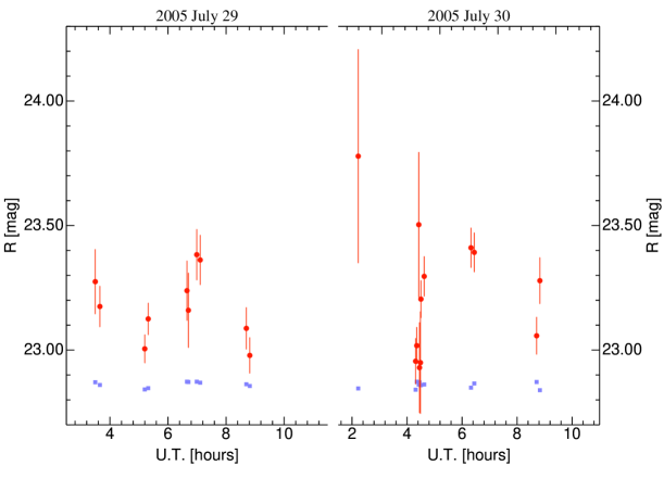
Figure 2: Light curves $R$ for Prospero. (See Fig. 1 for comments).

Fig.s 1, 2, 3, 4 and 5 presents $R$ light curves respectively for Sycorax, Prospero, Setebos, Stephano and Trinculo for the July 2005 nights. Each plot is splitted in two subpanels, the left for the July 29^th and the right for July 30^th. Squares in gray represents the measurements of a common field star with similar magnitude. To avoid confusion, error bars for the field star are not reported and the averaged magnitude is shifted. For the same reason the few data obtained in November 2005 for Prospero listed in the Tab.LABEL:tab:mag are not plotted in Fig. 2.

We analyse magnitude fluctuations in the light-curves trying to assess first of all whether the detected variations may be ascribed to random errors, Sect. 3.1, instabilities in the zero point of the calibration, Sect. 3.2, or to the effect of unresolved background objects Sect. 3.3. In case the variability has been judged significant attempt to estimate the amplitude and the period, Sect. 3.4. We use both analytical methods and a Monte Carlo (MC) – Bootstrap technique.

3.1 Testing against random fluctuations

The results of a $\chi^{2}$ test performed on V, R (and eventually B, I) measures are reported in the first two columns of Tab. 2 (similar results are obtained by a bootstrap on the data). In this test the hypothesis $H_{0}$ to be disproved is that the data are compatible with a constant signal (different from filter to filter) with random errors as the sole cause of brightness fluctuations. The table shows that this hypothesis may be discarded for Prospero and Sycorax with a very high level of confidence. As for Stephano and Setebos the level is lower but still significant, whereas for Trinculo the hypothesis can not be discarded at all. Before considering the case for a periodic variation, the case for a systematic trend in the brightness is considered, since the irregular sampling in time prevents the application of robust de-trendization techniques. As evident from the table, even this case can be excluded by the present data at a level of confidence similar to the constant case.

3.2 Field stars analysis

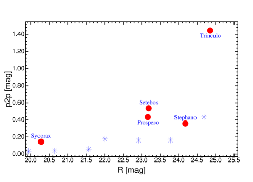
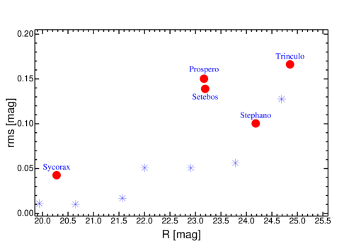
Figure 6: Variability of the $R$ light curves for irregular satellites (red circles) and field stars (light blue asterisks and gray band) as a function of their magnitude. Top frame for the peak–to–peak variation, bottom frame for RMS of the variation. (See the electronic edition of the Journal for a colour version of this figure).

In order to asses the level of calibration accuracy in an independent manner, several field stars having magnitudes encompassing those of the irregular satellites and common to each frame in both nights have been measured in the same way as the satellites (see Carraro et al., 2006, for an example of the adopted technique). As shown in Fig.s 1, 2, 3, 4 and 5 field stars are characterised by less wide fluctuations than satellites. A more quantitative test is obtained taking a set of variability indicators by which measuring the variability of field stars and satellites and comparing them. This is done in Fig. 6 where two variability indicators, the peak-to-peak variation (top) and the RMS (bottom), for satellites (red spots) and field stars (light blue asterisks) are plotted against the $R$ magnitude of the objects. The first important thing to note is the good consistency between the two indicators. While it is evident that the variability of Sycorax, Prospero and Setebos is above the level of variability of field stars, the same is not true for Stephano and Trinculo. In addition, test for the correlation of, as an example Sycorax or Prospero and the related field stars shows that they are not significantly correlated. As an example the correlation coefficient between Sycorax and three field stars is $C_{\mathrm{Sycorax},s}=-0.36$, $-0.08$ and $-0.53$. The probability that this level of correlation can be reached by chance even if their time series are not correlated are respectively $27\%$, $78\%$, $15\%$, while for Prospero $C_{\mathrm{Prospero},s}=-0.10$, $0.22$ and $-0.12$ with probabilities respectively of $64\%$, $36\%$ and $59\%$. In addition, even assuming a correlation between field stars fluctuations and satellite fluctuations, it would explain only a small fraction of the satellites variability. Indeed, variances of field stars accounts for $0.02\%-6\%$ of the Sycorax variance, $6\%-9\%$ of the Prospero variance, $12\%-18\%$ of the Setebos variance, $2\%-14\%$ of Stephano or Trinculo variances. In conclusion, field stars variability, connected to calibration instabilities, can not account for most of the variability of at least Sycorax, Prospero and Setebos, while as evident from Fig. 6 Stephano and Trinculo would have to be considered more cautiously.

3.3 Unresolved background objects

Unresolved objects in background may affect photometry. A quicklook to the frames shows that in general, the satellites passes far enough from background objects to allow a proper separation of their figures. It can be considered also the case in which a satellite crosses the figure of an undetected faint object in the background producing a fake time variability of the satellite light-curve. It is quite simple to compute the upper limit for the magnitude of a background object, $R_{\mathrm{bck}}$, able to produce the observed variations of magnitude for these satellites. The result is $\mbox{$R_{\mathrm{bck}}$}\leq 23.6$ mag, 24.7 mag, 25 mag, 25.5 mag and 25.5 mag, respectively for Sycorax, Prospero, Setebos, Stephano and Trinculo. Those magnitudes are within the detection limit for Sycorax and Prospero, near the detection limit for Setebos and marginally outside the detection limit for Stephano and Trinculo. In conclusion at least for Sycorax and Prospero, we can be confident that background is not important.

3.4 Looking for amplitudes and periodicities

Given the sparseness of our data it is not easy to asses safely the shapes, the amplitudes and the periods of our light-curves, despite at least for Sycorax, Prospero and probably Setebos a significant variability is present. However, we think important to attempt a recover of such informations, at least as a step toward planning of more accurate observations.

Constraints on the amplitude for the part of light curves sampled by our data may be derived from the analysis of the peak-to-peak variation. After excluding data with exposure times below 100 sec we evaluate peak–to–peak variations for R, $\Delta R_{\mathrm{p2p}}$. Denoting with $A_{\mathrm{R}}$ the amplitude of the light–curve we may assume $A_{\mathrm{R}}\approx\Delta R_{\mathrm{p2p}}/2$. To cope with the random noise, $\Delta R_{\mathrm{p2p}}$ have been evaluated by MonteCarlo, simulating the process of $\Delta R_{\mathrm{p2p}}$ evaluation assuming that the random errors of the selected data are normally distributed. We obtain $A_{\mathrm{R},\mathrm{Sycorax}}\ga 0.07\pm 0.01$ mag, $A_{\mathrm{R},\mathrm{Prospero}}\ga 0.27\pm 0.04$ mag and $A_{\mathrm{R},\mathrm{Setebos}}\ga 0.31\pm 0.05$ mag. Where the $\ga$ symbol is used because the $A_{\mathrm{R}}\approx\Delta R_{\mathrm{p2p}}/2$ relation is strictly valid only if the true minima and maxima of light–curves are sampled, a condition which we are not safe to have fullfilled. Another order of magnitude estimate of the amplitudes is based on the analysis of their RMS, $\mathrm{std}(R_{t})$. It easy to realize that for any periodical light-curve of amplitude $A_{\mathrm{R}}$ then $\mathrm{std}(R_{t})\approx f_{\mathrm{Dump}}\,A_{\mathrm{R}}$. Where $f_{\mathrm{Dump}}>0$ is a factor which depends both on the sampling function and the shape of signal. Assuming a sinusoidal signal sufficiently well sampled, $f_{\mathrm{Dump}}\approx 1.39-1.46$, giving for Sycorax $A_{\mathrm{R},\mathrm{Sycorax}}\approx 0.06$ mag, while for Prospero and Setebos $A_{\mathrm{R},\mathrm{Prospero}}\approx A_{\mathrm{R},\mathrm{Setebos}}\approx 0.2$ mag.

We then consider the case for a periodical variation in our light–curves by attempting first to search for the presence of periodicities in the hypothesys of a sinusoidal time dependence, and in case of a positive answer, assessing the most likely sinusoidal amplitude. To cope with the limited amount of data increasing both the sensitivity to weak variations and the discrimination power against different periods, we fit the same sinusoidal dependence on V, R (and eventually B and I) assuming that colours are not affected by any significant rotation effect. In short the model to be fitted is

$$M_{f}=A\cos({2\pi}/{P}(t-\tau)+\phi)+M_{f,0}\;,$$ (2)

where $f=$ R, V (and eventually B and I) indicates the filter, $M_{f}$ the measured magnitudes for that filter, $M_{f,0}$ the averaged magnitude for the filter $f$, $A$ is the amplitudes $\phi$ the phase and $\tau$ an arbitrary origin in time. It has to be noted that phase–angle effects are not considered here. The reason is that no safe dependence of the magnitude on the phase–angle has been established so far for these bodies. On the other hand, the variation of the phase angles over two consecutive nights is just about 2.4 arcmin. Consequently, we expect the phase–angle effect to be quite negligible. As widely discussed in literature the problem of searching for periodicities by fitting a model with a sinusoidal time dependence is equivalent to the analysis of the periodogram for the given data set (Lomb, 1976; Scargle, 1982; Cumming, Marcy & Butler, 1999; Cumming, 2004, just to cite some). The Lomb and Scargle (hereinafter LS) periodogram is the most used version. In this view, a better formulation of the problem is obtained expressing the model in the following form:

$$M_{f}=\mbox{$A_{\mathrm{c}}$}\cos\left(\frac{2\pi}{P}(t-\tau)\right)+\mbox{$A_{\mathrm{s}}$}\sin\left(\omega(t-\tau)\right)+M_{f,0}$$ (3)

where $\omega=\frac{2\pi}{P}$, $A_{\mathrm{c}}$ and $A_{\mathrm{s}}$ co-sinusoidal and sinusoidal amplitudes related to $A$ and $\phi$ by the simple relations $A=\sqrt{\mbox{$A_{\mathrm{c}}$}^{2}+\mbox{$A_{\mathrm{s}}$}^{2}}$ and phase $\phi=\arctan(\mbox{$A_{\mathrm{c}}$}/\mbox{$A_{\mathrm{s}}$})$. The time origin $\tau$ can be arbitrarily fixed, but the canonical choice is (Lomb, 1976; Scargle, 1982)

$$\tan(2\omega\tau)=\frac{\sum_{f=B,V,R,I}\sum_{j=1}^{N_{f}}\frac{\sin(\omega t_{f,j})}{\sigma^{2}_{f,j}}}{\sum_{f=B,V,R,I}\sum_{j=1}^{N_{f}}\frac{\cos(\omega t_{f,j})}{\sigma^{2}_{f,j}}}\;.$$ (4)

which will be our definition of $\tau$. Then, the free parameters involved in the minimisation are $P$, $M_{f,0}$ for $f=$V, R (B,I), $A_{\mathrm{c}}$ and $A_{\mathrm{s}}$ or equivalently, $A$ and $\phi$. However, being interested to amplitude and not to the phase we marginalise our statistics over $\phi$.

A set of best possible combinations of $M_{f,0}$ for $f=$V, R (B,I), $A_{\mathrm{c}}$ and $A_{\mathrm{s}}$ for each given $P$ in a suitable range $[\mbox{$P_{\mathrm{min}}$},\mbox{$P_{\mathrm{max}}$}]$ is obtained by minimising

$$\chi^{2}(P)=\sum_{f=B,V,R,I}\sum_{j=1}^{N_{f}}\frac{\left(\mbox{$A_{\mathrm{c}}$}\cos(\frac{2\pi}{P}(t_{f,j}-\tau))+\mbox{$A_{\mathrm{s}}$}\sin(\frac{2\pi}{P}(t_{f,j}-\tau))+M_{f,0}-m_{f,j}\right)^{2}}{\sigma^{2}_{f,j}},$$ (5)

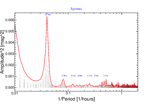
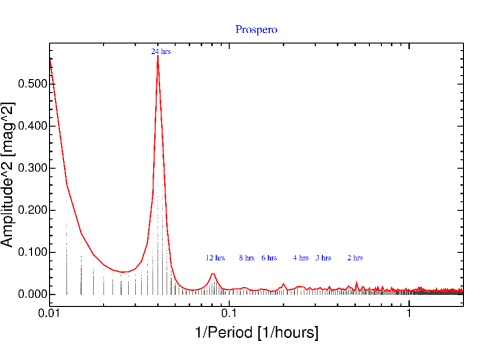
Figure 7: Time window for Sycorax (upper frame) and Prospero  (lower frame). (See the electronic edition of the Journal for a colour version of this figure).

where $m_{f,j}$ are the magnitudes for filter $f$ measured at the times $t_{f,j}$ with associated errors $\sigma_{f,j}$ with $j=1$, 2, $\dots$, $N_{f}$ the index of $N_{f}$ measures obtained for the filter $f$. The minimisation is carried out analytically, with the $\tau$ defined in Eq. (4). This way the method becomes a generalisation of the floating average periodogram (Cumming, Marcy & Butler, 1999; Cumming, 2004) and reduces to it in the case in which magnitudes come from a single filter, while in the case of homoscedastic data and null zero points we return to the classical LS periodogram.
The sensitivity to noise as a function of $P$ is not constant and varies with time. Fig. 7 represents the result for a Montecarlo designed to asses the sensitivity to noise of the periodogram in wide range of periods for Sycorax (upper frame) and Prospero (lower frame). The Montecarlo code generates simulated time series assuming the same time sampling of data, the same errors, normal distribution of errors and time independent expectations, and then computes the corresponding periodogram. Dots in the figure represents the realization of such periodograms, the full-line represents the Fourier transform of the time window. The sparseness of that causes a strong aliasing with diurnal periodicities. The plot is dominated by the prominent 24 hrs diurnal peak, followed by the 12 hrs, 8 hrs, 6 hrs, 4 hrs, 2 hrs peaks of decreasing amplitude. It is evident that above a period of 20 hrs the sensitivity of the periodogram to random errors is rapidly increasing. Then, our data set is best suited to detect periods below 20 hrs, or better, due to the presence of the 12 hrs peak, periods below 10 hrs.

Significant periodicities for $P<10$ hrs are likely present in the data if at least for one $P$ in the range, the squared amplitude $A^{2}(P)=\mbox{$A_{\mathrm{c}}$}^{2}(P)+\mbox{$A_{\mathrm{s}}$}^{2}(P)$ obtained by minimising Eq. (5), exceeds a critical value $A^{2}_{\mathrm{crit}}$, which is fixed by determining the false alarm probability for the given $[\mbox{$P_{\mathrm{min}}$},\mbox{$P_{\mathrm{max}}$}]$, $\mbox{$P_{\mathrm{FA}}$}(A^{2}>\mbox{$A^{2}_{\mathrm{crit}}$})$ . This interval has been sampled uniformly with a step size $\Delta P=0.025$ hours (the results do not depend much on the choice of the step size) and the $P_{\mathrm{FA}}$ as a function of $A^{2}_{\mathrm{crit}}$ has been assessed. In determining the $P_{\mathrm{FA}}$ we exploit the fact that we want to calculate this probability for values of $A^{2}_{\mathrm{crit}}$ for which $P_{\mathrm{FA}}$ is small. In this case,

$$\mbox{$P_{\mathrm{FA}}$}(A^{2}>\mbox{$A^{2}_{\mathrm{crit}}$})\approx\mbox{$P_{\mathrm{FA,0}}$}\exp(-\mbox{$A^{2}_{\mathrm{crit}}$}/\mbox{$A^{2}_{\mathrm{crit,0}}$}),$$ (6)

which is good for $\mbox{$P_{\mathrm{FA}}$}<0.3$, and with the parameters $P_{\mathrm{FA,0}}$ and $A^{2}_{\mathrm{crit,0}}$ determined from Montecarlo simulations. The last two columns of Tab. 2 report the results of this generalised version of the LS periodogram. Again, for Sycorax and Prospero a quite significant periodical signal is detected. For Setebos the detection is marginal, while for Stephano and Trinculo no detection can be claimed at all. There are many reasons for the lack of detections of periodicity despite random noise cannot account for the variability. Among them a lack in sensitivity, the fact that the period is outside the optimal search window, and that the light-curve cannot be described as a sinusoid. In conclusion, it is evident that a significant variability is present in most of these data sets and that for Sycorax and Prospero the July 2005 data suggests the possibility to construct a periodical light curve.

A period can be considered a good candidate if i.) $\chi^{2}(P)$ has a local minimum; ii.) the amplitude $A(P)$ of the associated sinusoid is significantly above the noise; iii.) the period $P$ is not affected in a significant manner by aliasing with the sampling window. Of course one has to consider the fact that one period may be preferred to another one just by chance. Random fluctuations may lead to a different selection of the best fit period. We assess this problem by generating random realizations of time series with expectation given by the measured values of each sample and $\sigma$ fixed by their Gaussian errors. For each generation the period producing the minimum $\chi^{2}(P)$ has been determined. The probability of selection of each $P$, $P_{\mathrm{sel}}(P)$, has been then derived. We then add a criterion iv) that a period $P$ is selected as most likely if it has the maximum $P_{\mathrm{sel}}(P)$. Tab. 3 reports the results of the fit. Note the difference in $\chi^{2}$ between the best fit with a sinusoid and the $\chi^{2}$ in Tab. 2.

Before looking at the results, it has to be stressed that light–curves can be either single peaked or double peaked. In the second case the rotation period will be twice the light – curve period. We have not enough data to discriminate between these two cases, therefore the rotational periods of the observed objects could be twice the light–curve periods.

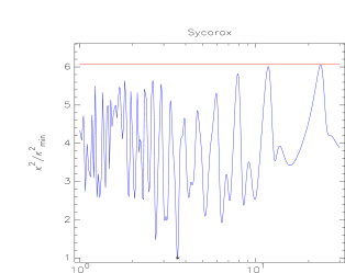
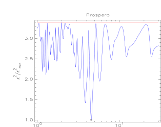
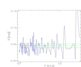
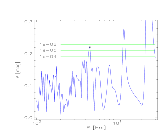
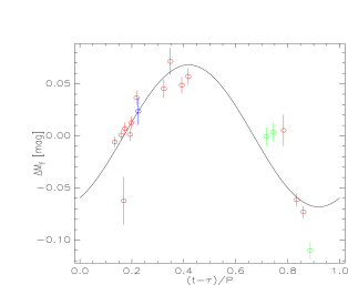
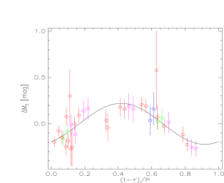
Figure 8: LS test of periodicity for Sycorax (left) and Prospero (right) light-curve as a function of the period $P$. Upper frames display $\chi^{2}/\chi^{2}_{\mathrm{min}}$, the red line is the $\chi^{2}/\chi^{2}_{\mathrm{min}}$ for the case of a constant signal. The central frames are the estimated amplitude, a group of green lines denotes the amplitudes for $\mbox{$P_{\mathrm{FA}}$}=10^{-4}$, $10^{-5}$, $10^{-6}$, $10^{-8}$ and $10^{-10}$. In all the frames a black $*$ marks the best fit point. Note that the diurnal $12$ hrs and $24$ hrs periods are excluded by the $\chi^{2}/\chi^{2}_{\mathrm{min}}$ despite the largest amplitude. The lower frames represents the overlap of the best reconstructed sinusoid with data ordered on a folded time scale, $(t-\tau)/P$, colours are blue for B, green for V, red for R and magenta for I.

Sycorax
Fig. 8 on the left is the periodogram for Sycorax. The $\chi^{2}$ suggests that the three periods $P\approx 3.6$, 3.1 and 2.8 hr are favoured with a very high level of confidence ($\mbox{$P_{\mathrm{FA}}$}<10^{-8}$). Bootstrap shows that the first period is the preferred one in about 96.6% of the simulations. The third period is chosen in less than 3.4% of the cases, the second one instead is chosen in less than 0.01% of the cases. For the best fit case we obtain also $B_{0}=21.676\pm 0.013$, $V_{0}=20.849\pm 0.005$, $R_{0}=20.276\pm 0.003$ which are compatible with the weighted averages discussed in the next section and are fairly independent of $P$. The same holds for the “derotated colours” $B_{0}-V_{0}=0.828\pm 0.014$, $V_{0}-R_{0}=0.573\pm 0.006$.

Prospero
Fig. 8  shows on the right the periodogram for Prospero. Given a safe dependence between the phase angle and magnitude is not established for these bodies, we just used the data taken on July 2005 to evaluate the periodogram. Four periods are allowed at a $5\sigma$ confidence level (c.l.) for $P\approx 4.6$, 3.8, 5.7 and and 3.3 hours, respectively. Bootstrap shows that the first peak is the preferred one in about 91% of the simulations. The second peak is chosen in less than 6% of the cases, the other peaks instead are chosen in less than 3% of the cases. Comparing the periodogram with the spectral window it is evident how the secondary peaks are close to alias of the diurnal 24 hr and 12 hr periods. Removing a 24 hr sinusoid from data before to perform the fit depresses the 24 hr peak, but not the 4.6 hr peak. On the contrary the removal of the 4.6 hr component strongly depresses the spectrum in the range $P\approx 3-8$ hr. By fitting separately the first and second night data, and avoiding the implicit 24 hr periodicity, the preferred period is 4.3 hr. Another way to filter the diurnal 24 hr periodicity is to shift in time the lightcurve of the second night to overlap the lightcurve of the first. Even in this case periods between 3 and 5 hours look favoured. The spectral window for the data shows a leakage corresponding to $P\approx 4.3$ hours. A secular variation may introduce power at periods longer than 48 hours which should leak power at $P\approx 4.3$ hours. The periodogram for simulated data with a linear time dependence has a peak in the $P\approx 4.3-4.6$ hours region, but in order to have an amplitude in the periodogram of 0.2 mag a peak-to-peak variation in the simulated data about seven or eight times larger than the peak-to-peak variation observed in real data is needed. Exclusion of B and/or I data, or fitting only the R data does not change significantly the results. The same holds if we remove the three R points with the largest errors. As a consequence, the data suggests $P\approx 4.6$ hr with $A\approx 0.21$ mag. The lower frame of Fig. 8 represents the variations of B, V, R and I magnitudes folded over the best fit sinusoid; For the best fit case we obtain also $B_{0}=24.584\pm 0.123$, $V_{0}=23.841\pm 0.053$, $R_{0}=23.202\pm 0.020$, $I_{0}=22.805\pm 0.043$ which are compatible with the weighted averages discussed in the next section and are fairly independent of $P$. The same holds for the “derotated colours” $B_{0}-V_{0}=0.743\pm 0.134$, $V_{0}-R_{0}=0.639\pm 0.057$, $R_{0}-I_{0}=0.397\pm 0.047$.

Setebos, Stephano and Trinculo
For the other three bodies no strong evidences are found for a periodicity in the present data. However for Setebos the data may be considered suggestive of some periodicity with $\mbox{$P_{\mathrm{FA}}$}\approx 0.7\%$, the preferred period being $P\approx 4.38\pm 0.05$ hours with $A\approx 0.189\pm 0.038$ mag. For Stephano and Trinculo best fit periods are $P_{\mathrm{Stephano}}\approx 2$ hours and $P_{\mathrm{Trinculo}}\approx 5.7$ hours with amplitudes $A_{\mathrm{Stephano}}\approx 0.459$ mag and $A_{\mathrm{Trinculo}}\approx 0.422$ hours but with $P_{\mathrm{FA}}$ of 22% and 44%, respectively.

4 Averaged Magnitudes and Colours

The derivation of colours would have to take in account the removal of rotational effects from magnitudes. Otherways systematic as large as peak–to–peak variations in the light–curve can be expected. Lacking a good light–curve we may apply two possible methods are: hierarchical determination of colours and compare weighted averages of magnitudes. The hierarchical method is based on the comparison of magnitudes from consecutive frames in the hypothesys that time differences are smaller than the light–curve period, so that rotational effects can be neglected. An example is the estimation of Setebos V-R by taking V3 and R15. In case in which one of the frames obtained with a given filter X is located between two frames of another filter Y, the Y magnitude at the epoch of which the X filter has been acquired can be derived by simple linear interpolation. An example is given by the estimate of V-R for Prospero in Nov 22, by interpolating R2 and R3 at the epoch of V1. Given in this way different estimates of each colours are obtained, weighted averages of such estimates are reported. The second method is based on the hypothesys that the light–curve has a periodical behaviour, and that it is so well sampled that weighting averages of magnitudes will cancell out the periodical time dependence. Of course the first method would be affected by larger random errors being based on a subset of the data. The second method is more prone to systematics.

Colours derived by using the first method for Sycorax, Prospero and Setebos are presented in Tab. 5. When more independent estimates of the same colour are possible their weighted average is taken.

Colours derived from the second method are listed in Tab. 4. The weighted averages of magnitudes for all of the satellites are listed in Tab. LABEL:tab:mag. In both cases, tables report just random errors and not the systematic calibration error, which amount to $0.018-0.022$ mag, depending on the filter.

It is evident how the results of the two methods are similar. Hence, we present for conciseness the results of the second one as commonly reported in literature.

Sycorax
We obtain $B-V=0.89\pm 0.01$ and $V-R=0.53\pm 0.01$, which are both compatible within 1$\sigma$ with the Maris et al. (2001) determinations but incompatible with Grav, Holman & Fraser (2004).

Prospero
We have two sets of colour measures for Prospero, one from the July and the other from the November run. We obtain $B-V=0.89\pm 0.13$, $V-R=0.63\pm 0.05$ and $R-I=0.40\pm 0.04$ from the July run, and $B-V=0.85\pm 0.13$, $V-R=0.59\pm 0.07$ and $R-I=0.33\pm 0.10$. The two set are consistent. With respect to Grav, Holman & Fraser (2004), we obtain a redder $V-R$, and a compatible $B-V$.

Setebos
We obtain $B-V=0.74\pm 0.14$ and $V-R=0.52\pm 0.04$. In this case Grav, Holman & Fraser (2004) obtained their data with the Keck II telescope and DEIMOS, which hosts a rather special filter set. Our $B-V$ is compatible with their, while as for Prospero our $V-R$ is redder.

Stephano and Trinculo
For these two extremely faint satellites, we could only derive the $V-R$ colour, which is $0.73\pm 0.17$ and $0.82\pm 0.43$ for Stephano and Trinculo, respectively. While our $V-R$ for Trinculo is in good agreement with Grav, Holman & Fraser (2004), their $V-R$ for Stephano is very low, and inconsistent with our one.

5 Summary and Conclusions

In this paper we report accurate photometric B, V, R, I observations obtained with the VLT telescope in two consecutive nights in July 2005 of the Uranian irregular satellites Sycorax, Stephano, Trinculo and Setebos. Additional observations of Prospero obtained in November 22 and 25 of the same year are also reported.

From the analysis of the data we conclude that Sycorax seems to displays a variability of $\approx 0.07$ mag, apparently larger than our previous result (Maris et al., 2001), while the period of 3.6 hr is in agreement with our previous 2001 determination, and the same is true for the colours, so it seems unlikely that the difference in amplitude can be ascribed to some systematic. If true, a possible explanation would be that in the two epochs two different parts of the same light curve have been sampled. But also it has to be noted that larger brightness variations have been not reported by other observers in the past years (Gladman et al., 1998; Rettig, Walsh & Consolmagno, 2001; Romon et al., 2001). Prospero light–curve exhibits an apparent periodicity of 4.6 hr and an amplitude of 0.21 mag. The impact of such a sizeable amplitude is throughly discussed in (Parisi et al., 2007). Colours for Prospero obtained in July and November are in a quite good agreement, further assessing the goodness of the relative calibration. Setebos colours are only in marginal agreement with previous studies. In addition the Setebos light curve displays a significant variability but it is not possible to asses a good fit using a simple sinusoidal time dependence. Wether this is due to undersampling of the light-curve or to a non-sinusoidal time dependence can not be decided from these data alone. However, assuming a sinusoidal time dependence, our data are suggestive of a light–curve amplitude of $\approx 0.18$ mag with a period of $\approx 4.4$ hours which will have to be confirmed or disproved by further observations. As for Stephano and Trinculo, the present data do not allow us to derive any sizeable time dependence, while the colours we derive are in marginal agreement with previous studies on the subject.

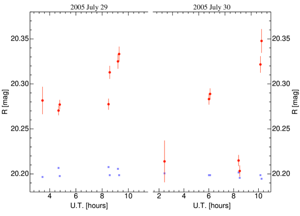
Figure 1: Light curves in $R$ for Sycorax. Data are for the nights of 2005, July 29^th (left) and 30^th (right). Squares in gray represents measurements of magnitudes for a common field star of similar magnitude. To avoid confusion error bars for the field star are not reported and the averaged magnitude is shifted. (See the electronic edition of the Journal for a colour version of this figure).

Figure 3: Light curves of Setebos. (See Fig. 1 for comments).

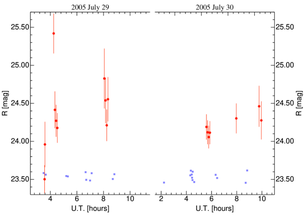
Figure 4: Light curves $R$ for Stephano. (See Fig. 1 for comments).

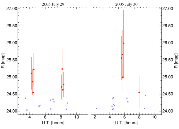
Figure 5: Light curves $R$ for Trinculo. (See Fig. 1 for comments).

Table 1: Log of observations. U.T. refers to the start times of exposures and are not corrected for light travel time. The Flt. column referes to the filter (BVRI) and frame number obtained with that filter (eg.: R3 is the third R frame for the given object in the serie). $T_{\mathrm{exp}}$ is the exposure time in seconds, the shortest exposures have been acquired to improve frame centering.

Obj	Epoch	U.T.	Flt.	$\stackrel{{\scriptstyle\mbox{$T_{\mathrm{exp}}$}}}{{[sec]}}$	mag
Sycorax	$\mathrm{Jul}\;29$	$03:27:13$	R1	30	$20.282\pm 0.015$
”	′′	$04:40:37$	R2	300	$20.270\pm 0.005$
”	′′	$04:46:05$	R3	300	$20.277\pm 0.005$
”	′′	$06:46:49$	V1	300	$20.849\pm 0.009$
”	′′	$06:52:17$	V2	300	$20.853\pm 0.009$
”	′′	$08:29:17$	R4	300	$20.277\pm 0.006$
”	′′	$08:34:45$	R5	300	$20.313\pm 0.007$
”	′′	$09:12:19$	R6	300	$20.325\pm 0.008$
”	′′	$09:17:47$	R7	300	$20.333\pm 0.008$
Sycorax	$\mathrm{Jul}\;30$	$02:26:25$	R8	30	$20.214\pm 0.023$
”	′′	$06:01:03$	R9	300	$20.283\pm 0.006$
”	′′	$06:06:29$	R10	300	$20.289\pm 0.006$
”	′′	$06:12:15$	B1	300	$21.701\pm 0.013$
”	′′	$08:24:01$	R11	300	$20.215\pm 0.006$
”	′′	$08:29:28$	R12	300	$20.203\pm 0.006$
”	′′	$08:35:07$	V3	300	$20.739\pm 0.008$
”	′′	$10:09:30$	R13	300	$20.322\pm 0.009$
”	′′	$10:14:56$	R14	300	$20.348\pm 0.013$
Stephano	$\mathrm{Jul}\;29$	$03:34:06$	R1	60	$23.502\pm 0.183$
”	′′	$03:35:34$	R2	60	$23.960\pm 0.297$
”	′′	$04:15:10$	R3	300	$25.419\pm 0.262$
”	′′	$04:20:37$	R4	300	$24.414\pm 0.242$
”	′′	$04:26:04$	R5	300	$24.271\pm 0.210$
”	′′	$04:31:31$	R6	300	$24.177\pm 0.195$
”	′′	$06:16:34$	V1	600	$25.033\pm 0.269$
Stephano	$\mathrm{Jul}\;29$	$06:27:02$	V2	600	$24.823\pm 0.295$
”	′′	$08:03:46$	R7	300	$24.827\pm 0.393$
”	′′	$08:09:14$	R8	300	$24.538\pm 0.299$
”	′′	$08:14:41$	R9	300	$24.211\pm 0.207$
”	′′	$08:20:09$	R10	300	$24.554\pm 0.291$
Stephano	$\mathrm{Jul}\;30$	$05:35:44$	R11	300	$24.190\pm 0.166$
”	′′	$05:41:11$	R12	300	$24.119\pm 0.157$
”	′′	$05:46:39$	R13	300	$24.056\pm 0.148$
”	′′	$05:52:07$	R14	300	$24.114\pm 0.151$
”	′′	$07:57:58$	R15	600	$24.302\pm 0.196$
”	′′	$08:08:36$	V3	600	$24.957\pm 0.290$
”	′′	$09:46:41$	R16	600	$24.285\pm 0.269$
”	′′	$09:57:11$	R17	600	$24.276\pm 0.250$
Setebos	$\mathrm{Jul}\;29$	$03:05:18$	R1	60	$23.230\pm 0.176$
”	′′	$03:54:07$	R2	300	$23.274\pm 0.088$
”	′′	$03:59:35$	R3	300	$23.337\pm 0.092$
”	′′	$04:05:03$	R4	300	$23.383\pm 0.092$
”	′′	$05:43:04$	V1	600	$23.796\pm 0.080$
”	′′	$05:53:32$	V2	600	$23.768\pm 0.083$
”	′′	$06:03:60$	V3	600	$23.781\pm 0.088$
”	′′	$07:29:43$	R5	600	$23.196\pm 0.080$
”	′′	$07:40:12$	R6	600	$23.242\pm 0.088$
”	′′	$07:50:40$	R7	600	$23.336\pm 0.099$
”	′′	$09:25:31$	R8	600	$23.100\pm 0.092$
”	′′	$09:35:58$	R9	600	$22.847\pm 0.074$
”	′′	$09:46:25$	R10	600	$22.903\pm 0.077$
Setebos	$\mathrm{Jul}\;30$	$02:16:30$	R11	60	$23.836\pm 0.318$
”	′′	$05:01:08$	R12	600	$23.272\pm 0.064$
”	′′	$05:11:37$	R13	600	$23.182\pm 0.062$
Setebos	$\mathrm{Jul}\;30$	$05:22:04$	R14	600	$23.314\pm 0.068$
”	′′	$07:02:39$	R15	600	$23.127\pm 0.061$
”	′′	$07:13:06$	R16	600	$23.205\pm 0.066$
”	′′	$07:23:51$	B1	600	$24.455\pm 0.132$
”	′′	$07:34:30$	V4	600	$23.649\pm 0.081$
”	′′	$07:44:58$	V5	600	$23.602\pm 0.075$
”	′′	$09:13:23$	R17	600	$23.223\pm 0.077$
”	′′	$09:23:50$	R18	600	$23.219\pm 0.078$
”	′′	$09:34:18$	R19	600	$23.249\pm 0.084$
Trinculo	$\mathrm{Jul}\;29$	$04:15:10$	R3	300	$25.110\pm 0.474$
”	′′	$04:20:37$	R4	300	$24.862\pm 0.378$
”	′′	$04:26:04$	R5	300	$24.544\pm 0.272$
”	′′	$04:31:31$	R6	300	$25.222\pm 0.485$
”	′′	$06:16:34$	V1	600	$25.925\pm 0.671$
”	′′	$06:27:02$	V2	600	$26.189\pm 0.901$
”	′′	$08:03:46$	R7	300	$24.711\pm 0.362$
”	′′	$08:09:14$	R8	300	$25.237\pm 0.568$
”	′′	$08:14:41$	R9	300	$24.626\pm 0.330$
”	′′	$08:20:09$	R10	300	$24.780\pm 0.361$
Trinculo	$\mathrm{Jul}\;30$	$05:35:44$	R11	300	$25.559\pm 0.631$
”	′′	$05:41:11$	R12	300	$25.664\pm 0.713$
”	′′	$05:46:39$	R13	300	$24.996\pm 0.386$
”	′′	$05:52:07$	R14	300	$25.988\pm 0.976$
”	′′	$07:57:58$	R15	600	$24.550\pm 0.465$
”	′′	$08:08:36$	V3	600	$25.167\pm 0.646$
Prospero	$\mathrm{Jul}\;29$	$03:29:44$	R1	100	$23.275\pm 0.130$
”	′′	$03:39:16$	R2	300	$23.175\pm 0.082$
”	′′	$03:46:44$	I1	300	$22.821\pm 0.117$
”	′′	$05:12:00$	R3	400	$23.005\pm 0.057$
Prospero	$\mathrm{Jul}\;29$	$05:19:09$	R4	400	$23.125\pm 0.064$
”	′′	$05:26:27$	V1	400	$23.680\pm 0.079$
”	′′	$05:33:34$	V2	400	$23.763\pm 0.085$
”	′′	$06:39:14$	R5	100	$23.239\pm 0.120$
”	′′	$06:42:09$	R6	50	$23.160\pm 0.150$
”	′′	$06:59:28$	R7	400	$23.383\pm 0.102$
”	′′	$07:06:36$	R8	400	$23.362\pm 0.100$
”	′′	$07:13:55$	I2	400	$22.996\pm 0.140$
”	′′	$07:21:03$	I3	400	$22.966\pm 0.144$
”	′′	$08:41:56$	R9	400	$23.087\pm 0.084$
”	′′	$08:49:04$	R10	400	$22.979\pm 0.072$
”	′′	$08:56:23$	I4	400	$22.552\pm 0.090$
”	′′	$09:03:30$	I5	400	$22.539\pm 0.089$
Prospero	$\mathrm{Jul}\;30$	$02:13:32$	R11	60	$23.779\pm 0.429$
”	′′	$04:18:45$	R12	98	$22.955\pm 0.092$
”	′′	$04:21:15$	R13	210	$23.018\pm 0.074$
”	′′	$04:25:37$	R14	20	$23.504\pm 0.291$
”	′′	$04:27:11$	R15	20	$22.929\pm 0.182$
”	′′	$04:29:12$	R16	20	$22.949\pm 0.205$
”	′′	$04:30:18$	R17	400	$23.205\pm 0.075$
”	′′	$04:37:26$	R18	400	$23.296\pm 0.080$
”	′′	$04:44:43$	I6	400	$22.947\pm 0.112$
”	′′	$04:51:51$	I7	400	$22.972\pm 0.114$
”	′′	$06:19:32$	R19	400	$23.411\pm 0.080$
”	′′	$06:26:39$	R20	400	$23.392\pm 0.079$
”	′′	$06:34:20$	B1	300	$24.622\pm 0.160$
”	′′	$06:39:48$	B2	300	$24.748\pm 0.180$
”	′′	$06:45:40$	V3	400	$23.867\pm 0.092$
”	′′	$06:52:47$	V4	400	$23.906\pm 0.101$
Prospero	$\mathrm{Jul}\;30$	$08:42:41$	R21	400	$23.057\pm 0.075$
”	′′	$08:49:48$	R22	400	$23.279\pm 0.093$
”	′′	$08:57:25$	I8	400	$22.792\pm 0.113$
”	′′	$09:04:32$	I9	400	$22.690\pm 0.103$
Prospero	$\mathrm{Nov}\;22$	$00:44:18$	R1	300	$23.193\pm 0.077$
”	′′	$00:50:04$	B1	300	$24.583\pm 0.181$
”	′′	$00:55:49$	R2	300	$23.240\pm 0.081$
”	′′	$01:01:27$	V1	300	$23.881\pm 0.110$
”	′′	$01:07:06$	R3	300	$23.310\pm 0.090$
”	′′	$01:12:45$	I1	300	$22.726\pm 0.157$
”	′′	$01:15:43$	I2	300	$22.925\pm 0.243$
”	′′	$01:18:52$	R4	300	$23.120\pm 0.076$
”	′′	$01:24:38$	B2	300	$24.710\pm 0.218$
”	′′	$01:30:25$	R5	300	$23.212\pm 0.083$
Prospero	$\mathrm{Nov}\;25$	$00:36:16$	V2	300	$23.835\pm 0.109$
”	′′	$00:41:54$	R6	300	$23.194\pm 0.080$
”	′′	$00:47:32$	I3	300	$22.838\pm 0.184$
”	′′	$00:50:29$	I4	300	$22.969\pm 0.207$
”	′′	$00:53:37$	R7	300	$23.279\pm 0.088$
”	′′	$00:59:23$	B3	300	$24.686\pm 0.203$
”	′′	$01:05:07$	R8	300	$23.063\pm 0.076$
”	′′	$01:10:45$	V3	300	$23.837\pm 0.108$
”	′′	$01:16:22$	R9	300	$23.284\pm 0.165$

Table 1: Continued.

Table 2: Testing against random fluctuations. Columns 2 - 3 $\chi^{2}$ and significativity level (SL) assuming constant signal, 4 - 5 $\chi^{2}$ and SL assuming linear time dependence, 6 - 7 maximum amplitude and false allarm probability assuming periodical signal. Note that in all the cases a low probability (either SL or $P_{\mathrm{FA}}$) denotes a high level of confidence in excluding noise fluctuations.

	Hypothesis H0
	Constant		Linear Trend		Periodical
Object	$\chi^{2}_{\mathrm{const}}$	SL	$\chi^{2}_{\mathrm{linear}}$	SL	$A_{\mathrm{max}}$	$P_{\mathrm{FA}}$
Sycorax	557	$<1\times 10^{-9}$	437	$<1\times 10^{-9}$	0.07	$<1\times 10^{-8}$
Prospero	92.7	$1\times 10^{-7}$	85.2	$1\times 10^{-6}$	0.22	$<3\times 10^{-6}$
Stephano	45.3	$4\times 10^{-4}$	44.9	$3\times 10^{-4}$	0.36	0.22
Setebos	59.2	$3\times 10^{-5}$	59.2	$2\times 10^{-5}$	0.19	$7\times 10^{-3}$
Trinculo	8.83	$8\times 10^{-1}$	8.44	$8\times 10^{-1}$	0.42	0.44

Table 3: Possible periods and amplitudes from fitting of Eq. 3. Column 1 $\chi^{2}$ for fitting, column 2 the confidence level (CL), Column 3 the best fit period in hours and its estimated internal uncertainty, Column 4 the corresponding amplitudes and their uncertainties. Solutions are ordered with increasing $\chi^{2}$.

Sycorax			$P$	$A$
#	$\chi^{2}$	CL	$[$hr$]$	$[$mag$]$
1	90.734	–	$3.60\pm 0.02$	$0.067\pm 0.004$
2	134.88	$2\sigma$	$2.70\pm 0.03$	$0.065\pm 0.003$
3	179.59	$3\sigma$	$3.04\pm 0.02$	$0.051\pm 0.010$
4	180.66	$3\sigma$	$3.13\pm 0.02$	$0.051\pm 0.010$
Prospero			$P$	$A$
#	$\chi^{2}$	CL	$[$hr$]$	$[$mag$]$
1	27.288	–	$4.551\pm 0.040$	$0.221\pm 0.027$
2	38.759	$2\sigma$	$3.827\pm 0.064$	$0.201\pm 0.029$
3	53.286	$3\sigma$	$5.760\pm 0.100$	$0.162\pm 0.090$
4	55.079	$3\sigma$	$3.300\pm 0.100$	$0.121\pm 0.090$

Table 4: Weighted averages of magnitudes

Obj	Run	B	V	R	I
Sycorax	Jul.	$21.701\pm 0.013$	$20.807\pm 0.005$	$20.276\pm 0.002$
Prospero	Jul.	$24.678\pm 0.120$	$23.788\pm 0.044$	$23.160\pm 0.019$	$22.760\pm 0.036$
Prospero	Nov.	$24.651\pm 0.115$	$23.851\pm 0.063$	$23.196\pm 0.028$	$22.864\pm 0.095$
Setebos	Jul.	$24.455\pm 0.132$	$23.713\pm 0.036$	$23.192\pm 0.018$
Stephano	Jul.		$24.944\pm 0.164$	$24.212\pm 0.050$
Trinculo	Jul.		$25.670\pm 0.413$	$24.855\pm 0.117$

Table 5: Colours derived from the hierarchical method

Obj	Run	B-V	V-R	R-I
Sycorax	Jul.	$0.915\pm 0.017$	$0.548\pm 0.006$
Prospero	Jul.	$0.793\pm 0.138$	$0.590\pm 0.056$	$0.395\pm 0.046$
Prospero	Nov.	$0.792\pm 0.171$	$0.635\pm 0.085$	$0.335\pm 0.131$
Setebos	Jul	$0.831\pm 0.143$	$0.444\pm 0.053$

Table 6: Colours derived from weigthed averages

Obj	Run	B-V	V-R	R-I
Sycorax	Jul.	$0.893\pm 0.014$	$0.531\pm 0.005$
Prospero	Jul.	$0.890\pm 0.127$	$0.628\pm 0.048$	$0.400\pm 0.041$
Prospero	Nov.	$0.800\pm 0.131$	$0.655\pm 0.069$	$0.332\pm 0.099$
Setebos	Jul.	$0.741\pm 0.137$	$0.522\pm 0.041$
Stephano	Jul.		$0.732\pm 0.171$
Trinculo	Jul.		$0.815\pm 0.430$