Good News for MOS, MXU & Co. – The New Spectroscopic Pipeline for the FORSes

Abstract

Since October 1, 2006, spectroscopic data from the two FORS instruments have been reduced with a new pipeline, which is based on a bottom-up calibration approach. I give a short description of the pipeline and discuss first experiences with automatic data reduction using this software, which has significantly increased the percentage of processed data for both instruments. I will also describe possible new options for Quality Control.

1 How does the Pipeline Work?

The spectroscopic pipeline for the FORS instruments can handle long-slit and multi-object spectroscopic data using slitlets. In order to be as flexible as possible most information is obtained directly from the observed calibration data, minimizing the need for assumptions (for details of the underlying principles see the contribution by Izzo et al.).

1.1 Calibration Data

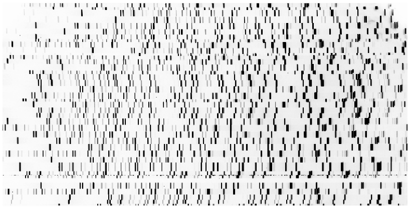
A first guess of the positions and lengths of the slitlets (or long slit) is obtained from an arc lamp frame (see Fig. 1). The positions of arc lamp spectra on the CCD are determined by a pattern matching technique applied to the detected emission lines. For that an estimate of the linear dispersion as well as a line catalog (which may both be provided by the user) are required. Adjacent slitlets with no offsets in dispersion direction are not distinguished and will form one longer slitlet.

Figure 1: Example of a raw arc frame for FORS2 MXU.

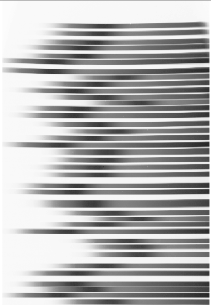
The spatial curvature is determined by tracing the edges of the corresponding flat field spectra (cf. Fig. 2) when possible. The curvature is fit by default with a second order polynomial. The final wavelength calibration is obtained taking into account the spatial curvature of the spectra.

The pipeline provides the following output calibration files:

• slit positions on the CCD at the central wavelength of the grism

• coefficients for the dispersion relation and the spatial curvature

• master bias

• master flat field (normalized and not-normalized)

• wavelength map and spatial map

• reduced arc lamp frame

• spectral resolution and line widths

The wavelength map specifies at the position of each original CCD pixel its corresponding wavelength. Thus the user can avoid the re-sampling of the spectra usually done after the wavelength calibration. The spatial map provides in the same manner the position of the CCD pixel within its associated slitlet. The reduced arc lamp frame allows to judge the quality of the calibration (straight arc lines, no wriggles, no offsets). If successful (see Sect. 2) the pipeline achieves an accuracy of 0.1 pixel both in spatial and dispersion direction.

Figure 2: Example of spatial curvature for a raw FORS2 MXU flat field.

1.2 Science Data

The default reduction of spectroscopic science data is as follows: The data are first corrected for bias. Then the extraction mask derived above (i.e. the positions of the slitlets and the curvatures of the resulting spectra) is applied to the science data; they are flat-fielded and re-mapped eliminating the optical distortions. Afterward they are rebinned to constant wavelength steps. The wavelength calibration can be adjusted using sky emission lines. This allows to correct for shifts between night-time science and day-time calibration data. Such shifts (of the order of 1 pixel) are known to happen due to flexure for MXU observations. Finally object spectra are detected and extracted, together with the corresponding error spectra and sky spectra. For long-slit spectroscopy the sky background is determined using a median. This is a valid approach if not more than half of the pixels contain flux from objects and there is no spatial gradient in the sky background. For multi-object spectroscopy instead the sky is subtracted before remapping, i.e. when the spectra are still in the original CCD coordinate system. The sky is determined with a robust linear fitting, which allows for a linear spatial gradient in the background. Also in this case, however, not more than half of the pixels may contain flux from the object(s).

The output science files are

• positions and widths of object spectra

• extracted object spectra, error spectra, and sky spectra

• unmapped (corrected for spatial distortions, not rebinned) science frames

• mapped (i.e. corrected for spatial distortions and rebinned) science frames

• adjusted dispersion coefficients and wavelength map

2 Strengths and Weaknesses

The major strength of the new pipeline is its flexibility and robustness. It requires only very limited input information (mainly dispersion estimate and line catalog) and can therefore be applied to a large variety of instrument configurations. Thus it is now possible for the first time to automatically reduce long-slit (LSS) and multi-object spectroscopic data (MOS/MXU) from the two FORS instruments for all grisms and both collimators (standard and high-resolution). To verify its flexibility the pipeline was applied to data from the Low-Resolution Spectrograph of the Hobby Eberly Telescope, which it handled without any problems.

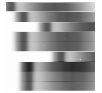
The pipeline does have problems if there are too few arc lines, e.g. for slitlets with large offsets. In such cases it sometimes fails to correctly identify the slitlet. This can be most easily recognized by comparing the not-normalized and the normalized screen flat (cf. Fig. 3 – one slitlet is partly missing, another one was not processed at all). Large gaps between arc lines can be problematic as non-linear dispersion terms can become important, while the pipeline currently uses only linear dispersion estimates for the pattern matching.

Figure 3: Example of missed slitlets in FORS2 MOS data (left: averaged screen flat, right: normalized screen flat).

The pipeline will fail in case of regularly spaced arc lines, like those created by a laser comb, as its pattern matching (see contribution by Izzo et al.) does not work for such data.

3 Quality Control

In order to check the quality of observational data a pipeline is of great importance. Otherwise it is difficult to distinguish between well-known and correctable instrument effects and real problems. Quality control shall ensure that the data observed with the FORSes can be calibrated. In addition the trending of certain parameters allows to have an eye on the instrument health (see http://www.eso.org/dfo/quality for more details). Therefore the resolution, central wavelength, and number of identified arc lines are regularly monitored. A change in the number of identified lines can indicate reduced flux of the arc lamp and possibly impending failure of the lamp. A change in resolution could indicate focus problems.

Figure 4: Curvature coefficients for FORS2 MXU data for the 600z grism. The lower branch resulting from chip 2 data indicates that chip 2 is mounted at an angle of 0$\stackrel{{\scriptstyle\circ}}{{.}}$079$\pm$ 0$\stackrel{{\scriptstyle\circ}}{{.}}$007 with respect to chip 1 (the known value being 0$\stackrel{{\scriptstyle\circ}}{{.}}$083). The reduced arc lamp image corresponding to the coefficients in the dashed box is shown in Fig. 5

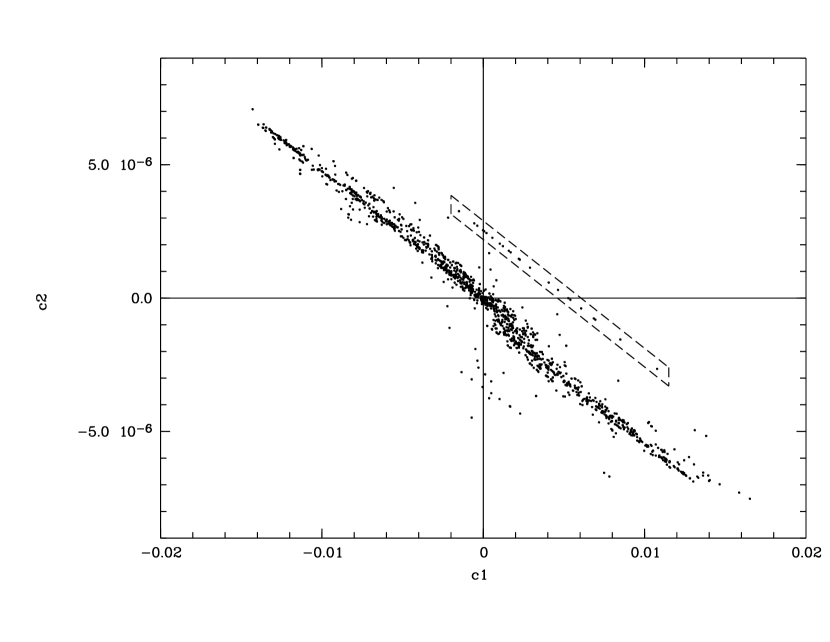
The situation for the quality control of FORS data has vastly improved with the new pipeline, as now almost all data can be reduced (with polarimetric data being the only exception). Moreover, the new pipeline also provides additional information on the instrument. For example, the combination of the curvature coefficients can be used to monitor grism alignment: The coefficients c1 and c2 describe the slope and the curvature of a slitlet, respectively. If the curvature is 0, then the slope should be 0 as well – otherwise this indicates that the grism is not well aligned. Fig. 4 shows the coefficients obtained for the 600z FORS2 grism. Obviously the correlation for the majority of solutions passes through zero.

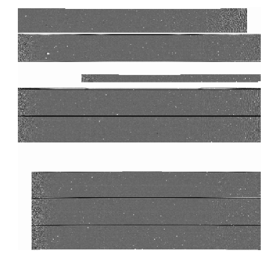
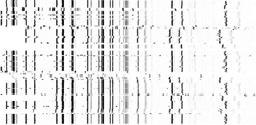
Some solutions, however, show significant offsets from the general trend. Fig. 5 shows a reduced arc lamp image for such a deviating case (marked by the dashed box in Fig. 4). Obviously the wavelength calibration obtained for several slitlets is rather bad (wriggles instead of straight lines). Thus diagrams like Fig. 4 allow to look for bad solutions efficiently in case of large data volume, which may prohibit checking all solutions individually.

Figure 5: Reduced arc lamp frame for the deviating points marked in Fig. 4.

Other new parameters become available if there are more than 12 slitlets distributed across the CCD. In this case the pipeline calculates a global distortion model, which contains good indicators for the monitoring of the instrument’s health, like the instrument scale.

4 Concluding Remarks

The new spectroscopic pipeline for the FORS instruments has been a great success in that it allows to reduce automatically long-slit and multi-object spectroscopic data for all FORS grisms. The fact that it does not need a first guess from an instrument model makes it a promising candidate for the reduction of spectroscopic data from a variety of instruments. In addition this approach is extremely helpful in the presence of instrument instabilities as it allows to reduce data whose configurations deviate from the expected one (e.g. due to instrument aging or earthquakes).