Large System Analysis of Game-Theoretic Power Control in UWB Wireless Networks with Rake Receivers

Abstract

This paper studies the performance of partial-Rake (PRake) receivers in impulse-radio ultrawideband wireless networks when an energy-efficient power control scheme is adopted. Due to the large bandwidth of the system, the multipath channel is assumed to be frequency-selective. By using noncooperative game-theoretic models and large system analysis, explicit expressions are derived in terms of network parameters to measure the effects of self- and multiple-access interference at a receiving access point. Performance of the PRake is compared in terms of achieved utilities and loss to that of the all-Rake receiver.

1 Introduction

Ultrawideband (UWB) technology is considered to be a potential candidate for next-generation multiuser data networks, due to its large spreading factor (which implies large multiuser capacity) and its lower spectral density (which allows coexistence with incumbent systems). The requirements for designing high-speed data mobile terminals include efficient resource allocation and interference reduction. These issues aim to allow each user to achieve the required quality of service at the uplink receiver without causing unnecessary interference to other users in the system, and minimizing power consumption. Scalable energy-efficient power control (PC) techniques can be derived using game theory [1, 2].

In this work, performance of partial Rake (PRake) receivers [3] is studied in terms of transmit powers and utilities achieved in the uplink of an infrastructure network at the Nash equilibrium, where utility here is defined as the ratio of throughput to transmit power. By using the large system analysis proposed in [2], we obtain a general characterization for the terms due to self-interference (SI) and multiple access interference (MAI). Explicit expressions for the utilities achieved at the Nash equilibrium are then derived, and an approximation for the loss of PRake receivers with respect to (wrt) all-Rake (ARake) receivers is proposed.

The remainder of the paper is organized as follows. Some background for this work is given in Sect. 2, where the system model and the results of the game-theoretic PC approach are shown. In Sect. 3, large system analysis is used to evaluate the effects of the interference at the Nash equilibrium. Performance of the PRake at the Nash equilibrium is analyzed in Sect. 4, where also a comparison with simulations is provided. Some conclusions are drawn in Sect. 5.

2 Background

2.1 System Model

Commonly, impulse-radio (IR) systems are employed to implement UWB systems. We focus here on a binary phase shift keying (BPSK) time hopping (TH) IR-UWB system with polarity randomization [4]. A network with $K$ users transmitting to a common concentration point is considered. The processing gain is $N=N_{f}\cdot N_{c}$, where $N_{f}$ is the number of pulses that represent one information symbol, and $N_{c}$ is the number of possible pulse positions in a frame [4]. The transmission is assumed to be over frequency selective channels, with the channel for user $k$ modeled as a tapped delay line:

$$c_{[}(k)]{t}=\sum_{l=1}^{L}{\alpha_{[}^{(l)}]{k}\delta(t-(l-1)T_{c}-\tau_{[}k])},$$ (1)

where $T_{c}$ is the duration of the transmitted UWB pulse; $L$ is the number of channel paths; $\mbox{\boldmath$\alpha$}_{[}k]=[\alpha_{[}^{(1)}]{k},\dots,\alpha_{[}^{(L)}]{k}]^{T}$ and $\tau_{[}k]$ are the fading coefficients and the delay of user $k$, respectively. Considering a chip-synchronous scenario, the symbols are misaligned by an integer multiple of $T_{c}$: $\tau_{[}k]=\Delta_{k}T_{c}$, for every $k$, where $\Delta_{k}$ is uniformly distributed in $\{0,1,\dots,N-1\}$. In addition, we assume that the channel characteristics remain unchanged over a number of symbol intervals [4].

Due to high resolution of UWB signals, multipath channels can have hundreds of components, especially in indoor environments. To mitigate the effect of multipath fading as much as possible, we consider an access point where $K$ Rake receivers[3] are used. The Rake receiver for user $k$ is in general composed of $L$ coefficients, where the vector $\mbox{\boldmath$\beta$}_{[}k]=\mathbf{G}\cdot\mbox{\boldmath$\alpha$}_{[}k]=[\beta_{[}^{(1)}]{k},\dots,\beta_{[}^{(L)}]{k}]^{T}$ represents the combining weights for user $k$, and the $L\times L$ matrix $\mathbf{G}$ depends on the type of Rake receiver employed. In particular, if $\{\mathbf{G}\}_{ll}=1$ for $1\leq l\leq r\cdot L$, and $0$ elsewhere, where $r\triangleq L_{P}/L$ and $0<L_{P}\leq L$, a PRake with $L_{P}$ fingers using maximal ratio combining (MRC) scheme is considered. It is worth noting that, when $r=1$, an ARake is implemented.

The signal-to-interference-plus-noise ratio (SINR) of the $k$th user at the output of the Rake receiver can be well approximated (for large $N_{f}$, typically at least 5) by [4]

$$\gamma_{[}k]=\frac{h_{[}^{(\text{SP})}k]p_{[}k]}{\displaystyle{h_{[}^{(\text{SI})}k]p_{[}k]+\sum_{j\neq k}{h_{[}^{(\text{MAI})}kj]p_{[}j]}+\sigma^{2}}},$$ (2)

where $\sigma^{2}$ is the variance of the additive white Gaussian noise (AWGN) at the receiver; $p_{[}k]$ denotes the transmit power of user $k$; and the gains are expressed by

$$h_{[}^{(\text{SP})}k] =\mbox{\boldmath$\beta$}_{[}k]^{H}\cdot\mbox{\boldmath$\alpha$}_{[}k],$$ (3)

$$h_{[}^{(\text{SI})}k] =\frac{1}{N}\frac{\left|\left|{\bm{\Phi}\cdot\left(\mathbf{B}_{[}k]^{H}\cdot\mbox{\boldmath$\alpha$}_{[}k]+\mathbf{A}_{[}k]^{H}\cdot\mbox{\boldmath$\beta$}_{[}k]\right)}\right|\right|^{2}}{\mbox{\boldmath$\beta$}_{[}k]^{H}\cdot\mbox{\boldmath$\alpha$}_{[}k]},$$ (4)

$$h_{[}^{(\text{MAI})}kj] =\frac{1}{N}\frac{\left|\left|{\mathbf{B}_{[}k]^{H}\cdot\mbox{\boldmath$\alpha$}_{[}j]}\right|\right|^{2}+\left|\left|{\mathbf{A}_{[}j]^{H}\cdot\mbox{\boldmath$\beta$}_{[}k]}\right|\right|^{2}+\left|\mbox{\boldmath$\beta$}_{[}k]^{H}\cdot\mbox{\boldmath$\alpha$}_{[}j]\right|^{2}}{\mbox{\boldmath$\beta$}_{[}k]^{H}\cdot\mbox{\boldmath$\alpha$}_{[}k]},$$ (5)

where the matrices

$$\mathbf{A}_{[}k] =\begin{pmatrix}\alpha_{[}^{(L)}]{k}&\cdots&\cdots&\alpha_{[}^{(2)}]{k}\\ 0&\alpha_{[}^{(L)}]{k}&\cdots&\alpha_{[}^{(3)}]{k}\\ \vdots&\ddots&\ddots&\vdots\\ 0&\cdots&0&\alpha_{[}^{(L)}]{k}\\ 0&\cdots&\cdots&0\end{pmatrix},$$ (6)

$$\mathbf{B}_{[}k] =\begin{pmatrix}\beta_{[}^{(L)}]{k}&\cdots&\cdots&\beta_{[}^{(2)}]{k}\\ 0&\beta_{[}^{(L)}]{k}&\cdots&\beta_{[}^{(3)}]{k}\\ \vdots&\ddots&\ddots&\vdots\\ 0&\cdots&0&\beta_{[}^{(L)}]{k}\\ 0&\cdots&\cdots&0\end{pmatrix},$$ (7)

$$\bm{\Phi} =\operatorname{diag}\left\{\phi_{[}1],\dots,\phi_{[}L-1]\right\},\quad\phi_{[}l]=\sqrt{\tfrac{\min\{L-l,N_{c}\}}{N_{c}}},$$ (8)

have been introduced for convenience of notation.

2.2 The Game-Theoretic Power Control Game

Consider the application of noncooperative PC techniques to the wireless network described above. Focusing on mobile terminals, where it is often more important to maximize the number of bits transmitted per Joule of energy consumed than to maximize throughput, a game-theoretic energy-efficient approach as the one described in [2] is considered.

We examine a noncooperative PC game in which each user seeks to maximize its own utility function as follows. Let $G=[\mathcal{K},\{P_{[}k]\},\{u_{[}(k)]{\mathbf{p}_{[}]}\}]$ be the proposed game where $\mathcal{K}=\{1,\dots,K\}$ is the index set for the users; $P_{[}k]=[0,\overline{p}_{[}]]$ is the strategy set, with $\overline{p}_{[}]$ denoting the maximum power constraint; and $u_{[}(k)]{\mathbf{p}_{[}]}$ is the payoff function for user $k$ [1]:

$$u_{[}(k)]{\mathbf{p}_{[}]}=\frac{D}{M}R_{[}]\frac{f([){\gamma_{[}k]}]}{p_{[}k]},$$ (9)

where $\mathbf{p}_{[}]=[p_{[}1],\dots,p_{[}K]]$ are the transmit powers; $D$ is the number of information bits per packet; $M$ is the total number of bits per packet; $R_{[}]$ is the transmission rate; $\gamma_{[}k]$ is the SINR (2) for user $k$; and $f([){\gamma_{[}k]}]$ is the efficiency function representing the packet success rate (PSR), i.e., the probability that a packet is received without an error.

When the efficiency function is increasing, S-shaped [1], and continuously differentiable, with $f([)0]=0$, $f([)+\infty]=1$, $f^{\prime}([)0]=df([){\gamma_{[}k]}]/d\gamma_{[}k]|_{\gamma_{[}k]=0}=0$, it has been shown [2] that the solution of the maximization problem $\max_{p_{[}k]\in P_{[}k]}u_{[}(k)]{\mathbf{p}_{[}]}$ is

$$p^{*}_{[}k]=\min\left\{\frac{\gamma^{*}_{[}k]\left(\sum_{j\neq k}{h_{[}^{(\text{MAI})}kj]p_{[}j]}+\sigma^{2}\right)}{h_{[}^{(\text{SP})}k]\left(1-\gamma^{*}_{[}k]/\gamma_{0,{[}}k]\right)},\overline{p}_{[}]\right\},$$ (10)

where $\gamma^{*}_{[}k]$ is the solution of

$$f^{\prime}([){\gamma^{*}_{[}k]}]\gamma^{*}_{[}k]\left(1-\gamma^{*}_{[}k]/\gamma_{0,{[}}k]\right)=f([){\gamma^{*}_{[}k]}],$$ (11)

with $f^{\prime}([){\gamma^{*}_{[}k]}]=df([){\gamma_{[}k]}]/d\gamma_{[}k]|_{\gamma_{[}k]=\gamma^{*}_{[}k]}$, and $\gamma_{0,{[}}k]=h_{[}^{(\text{SP})}k]/h_{[}^{(\text{SI})}k]$.

$$\nu\left({[}\right){\Lambda,r,\rho}]=\begin{cases}\tfrac{\Lambda\left(\Lambda^{\rho}-1\right)\left(4\Lambda^{2r}+3\Lambda^{\rho}-1\right)-2\Lambda^{r+\rho}\left(\Lambda^{r}+3\Lambda-1\right)\rho\log{\Lambda}}{2\left(\Lambda^{r}-1\right)^{2}\rho\Lambda^{1+\rho}\log{\Lambda}},&\text{if $0\leq\rho\leq\min(r,1-r)$};\\ \tfrac{\Lambda\left(4\Lambda^{\rho}-1\right)\left(\Lambda^{2r}-1\right)-2\Lambda^{r+\rho}\left(3\Lambda r-\rho+\Lambda^{r}\rho\right)\log{\Lambda}}{2\left(\Lambda^{r}-1\right)^{2}\rho\Lambda^{1+\rho}\log{\Lambda}},&\text{if $r\leq\rho\leq 1-r$ and}\\ &\,\,\,\,\,\,\text{$r\leq 1/2$};\\ \tfrac{-4\Lambda^{2+2r}-4\Lambda^{2+\rho}+\Lambda^{2(r+\rho)}+4\Lambda^{2+2r+\rho}+3\Lambda^{2+2\rho}-2\Lambda^{1+r+\rho}\left(r+3\Lambda\rho+\Lambda^{r}\rho-1\right)\log{\Lambda}}{2\left(\Lambda^{r}-1\right)^{2}\rho\Lambda^{2+\rho}\log{\Lambda}},&\text{if $1-r\leq\rho\leq r$ and}\\ &\,\,\,\,\,\,\text{$r\geq 1/2$};\\ \tfrac{-\Lambda^{2+2r}-4\Lambda^{2+\rho}+\Lambda^{2(r+\rho)}+4\Lambda^{2+2r+\rho}-2\Lambda^{1+r+\rho}\left(r+3\Lambda\rho+\Lambda^{r}\rho-1\right)\log{\Lambda}}{2\left(\Lambda^{r}-1\right)^{2}\rho\Lambda^{2+\rho}\log{\Lambda}}&\text{if $\max(r,1-r)\leq\rho\leq 1$};\\ \tfrac{2\Lambda\left(\Lambda^{2r}-1\right)-\left(\Lambda^{r}+r+3\Lambda r-1\right)\Lambda^{r}\log{\Lambda}}{\left(\Lambda^{r}-1\right)^{2}\rho\Lambda\log{\Lambda}},&\text{if $\rho\geq 1$}.\end{cases}$$ (17)

In the typical case of multiuser UWB systems, $N\gg K$. If $\overline{p}_{[}]$ is sufficiently large, (10) can be reduced to [2]

$$p^{*}_{[}k]=\frac{1}{h_{[}^{(\text{SP})}k]}\cdot\frac{\sigma^{2}\overline{\gamma_{[}]}^{*}}{1-\overline{\gamma_{[}]}^{*}\cdot\left(\gamma_{0,{[}}k]^{-1}+\zeta_{[}k]^{-1}\right)},$$ (12)

where $\zeta_{[}k]^{-1}=\sum_{j\neq k}{h_{[}^{(\text{MAI})}kj]/h_{[}^{(\text{SP})}j]}$; and $\overline{\gamma_{[}]}^{*}$ is the SINR at the Nash equilibrium in the absence of SI, i.e., it is the solution of (11) when $\gamma_{0,{[}}k]=+\infty$.

A necessary and sufficient condition for the Nash equilibrium to be achieved simultaneously by all the $K$ users, and thus for (12) to be valid, is [2]

$$\overline{\gamma_{[}]}^{*}\cdot\left(\gamma_{0,{[}}k]^{-1}+\zeta_{[}k]^{-1}\right)<1\quad\forall k\in\mathcal{K}.$$ (13)

3 Analysis of the Interference

3.1 Analytical Results

As can be verified in (12), the amount of transmit power $p^{*}_{[}k]$ required to achieve the target SINR $\gamma^{*}_{[}k]$ will depend not only on the gain $h_{[}^{(\text{SP})}k]$, but also on the SI term $h_{[}^{(\text{SI})}k]$ (through $\gamma_{0,{[}}k]$) and the interferers $h_{[}^{(\text{MAI})}kj]$ (through $\zeta_{[}k]$). To derive quantitative results for the transmit powers independent of SI and MAI terms, it is possible to resort to a large-system analysis [2].

For ease of calculation, the expressions derived in the remainder of the paper consider the following assumptions:

• The channel gains are assumed to be independent complex Gaussian random variables with zero mean and variance $\sigma^{2}_{{[}}{k_{l}}]$, i.e., $\alpha_{[}^{(k)}]{l}\sim\mathcal{CN}(0,\sigma^{2}_{{[}}{k_{l}}])$. This assumption leads $|\alpha_{[}^{(k)}]{l}|$ to be Rayleigh-distributed with parameter $\sigma^{2}_{{[}}{k_{l}}]/2$. Although channel modeling for UWB systems is still an open issue, this hypothesis, appealing for its analytical tractability, also provides a good approximation for multipath propagation in UWB systems [5].

• The averaged power delay profile (aPDP) is assumed to decay exponentially, as is customarily taken in most UWB channel models [6]. Hence, $\sigma^{2}_{{[}}{k_{l}}]=\sigma^{2}_{{[}}k]\cdot\Lambda^{-\frac{l-1}{L-1}}$, where $\Lambda=\sigma^{2}_{{[}}{k_{1}}]/\sigma^{2}_{{[}}{k_{L}}]$ and $\sigma^{2}_{{[}}k]$ depends on the distance between user $k$ and the base station. It is easy to verify that $\Lambda=0\,\text{dB}$ represents the case of flat aPDP.

Prop. 1

In the asymptotic case where $K$ and $N_{f}$ are finite, while $L,N_{c}\rightarrow\infty$, when adopting a PRake with $L_{P}$ coefficients according to the MRC scheme, the terms $\zeta_{[}k]^{-1}$ and $\gamma_{0,{[}}k]^{-1}$ converge almost surely (a.s.) to

$$\zeta_{[}k]^{-1} \stackrel{{\scriptstyle a.s.}}{{\rightarrow}}\frac{K-1}{N}\cdot\mu\left({[}\right){\Lambda,r}],$$ (14)

$$\gamma_{0,{[}}k]^{-1} \stackrel{{\scriptstyle a.s.}}{{\rightarrow}}\frac{1}{N}\cdot\nu\left({[}\right){\Lambda,r,\rho}],$$ (15)

where $$r\triangleq L_{P}/L 0<r\leq 1 \rho\triangleq N_{c}/L 0<\rho<\infty$$, , and , , are held constant, and

$$\mu\left({[}\right){\Lambda,r}] =\frac{\left(\Lambda-1\right)\cdot\Lambda^{r-1}}{\Lambda^{r}-1},$$ (16)

with $\nu\left({[}\right){\Lambda,r,\rho}]$ defined as in (17), shown at the top of the page.

The proof of Prop. 1 has been omitted because of space limitation. It can be found in [7].

Proposition 1 gives accurate approximations for the terms of MAI and SI in the case of PRake receivers at the access point and of exponentially decaying aPDP. Results for more specific scenarios can be derived using particular values of $\Lambda$ and $r$, as shown in [7]. As an example, it is possible to obtain approximations for the MAI and SI arising in the ARake as follows:

$$\mu_{A}\left({[}\right)\Lambda]=\lim_{r\to 1}\mu\left({[}\right){\Lambda,r}]=1,$$ (18)

$$\nu_{A}\left({[}\right){\Lambda,\rho}]=\lim_{r\to 1}\nu\left({[}\right){\Lambda,r,\rho}]=$$

$$\quad=\begin{cases}\displaystyle{\frac{2\left(\Lambda^{2}-1+\Lambda^{\rho}-\Lambda^{2-\rho}-2\Lambda\rho\log{\Lambda}\right)}{\left(\Lambda-1\right)^{2}\rho\log{\Lambda}}},&\text{if $\rho\leq 1$},\\ \displaystyle{\frac{2\left(\Lambda^{2}-1-2\Lambda\log{\Lambda}\right)}{\left(\Lambda-1\right)^{2}\rho\log{\Lambda}}},&\text{if $\rho\geq 1$}.\end{cases}$$ (19)

3.2 Comments on the Results

Fig. 1 shows the shape of $\mu\left({[}\right){\Lambda,r}]$ versus $r$ for some values of $\Lambda$. As can be noticed, $\mu\left({[}\right){\Lambda,r}]$ is decreasing as either $\Lambda$ or $r$ increases. Keeping $r$ fixed, $\mu\left({[}\right){\Lambda,r}]$ is a decreasing function of $\Lambda$, since the neglected paths are weaker as $\Lambda$ increases. Keeping $\Lambda$ fixed, $\mu\left({[}\right){\Lambda,r}]$ is a decreasing function of $r$, since the receiver uses a higher number of coefficients, thus better mitigating the effect of MAI.

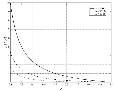
Fig. 1: Shape of $\mu\left({[}\right){\Lambda,r}]$ versus $r$ for some $\Lambda$’s.

Fig. 2 shows the shape of $\nu\left({[}\right){\Lambda,r,\rho}]$ versus $r$ for some values of $\Lambda$ and $\rho$. As can be verified, $\nu\left({[}\right){\Lambda,r,\rho}]$ decreases as either $\rho$ or $\Lambda$ increases. This dependency of $\nu\left({[}\right){\Lambda,r,\rho}]$ wrt $\rho$ is justified by the higher resistance to multipath due to increasing the length of a single frame [2, 4]. Similarly to $\mu\left({[}\right){\Lambda,r}]$, $\nu\left({[}\right){\Lambda,r,\rho}]$ is a decreasing function of $\Lambda$ when $r$ and $\rho$ are fixed, since the neglected paths are weaker as $\Lambda$ increases. Taking into account the dependency of $\nu\left({[}\right){\Lambda,r,\rho}]$ wrt $r$, it can be verified that $\nu\left({[}\right){\Lambda,r,\rho}]$ is not monotonically decreasing as $r$ increases. In other words, an ARake receiver using MRC does not offer the optimum performance in mitigating the effect of SI, but it is outperformed by PRake receivers whose $r$ decreases as $\Lambda$ increases. This behavior is due to using MRC, which attempts to gather all the signal energy to maximize the signal-to-noise ratio (SNR) and substantially ignores the SI. In this scenario, a minimum mean square error (MMSE) combining criterion, while more complex, might give a different comparison.

4 Analysis of the Nash Equilibrium

4.1 Analytical Results

Using Prop. 1 in (9) and (12), it is straightforward to obtain the utilities $u^{*}_{[}k]$ at the Nash equilibrium, which are independent of the channel realizations of the other users, and of SI:

$$u^{*}_{[}k] \stackrel{{\scriptstyle a.s.}}{{\rightarrow}}h_{[}^{(\text{SP})}k]\cdot\frac{D}{M}R_{[}]\frac{f([){\overline{\gamma_{[}]}^{*}}]}{\sigma^{2}\overline{\gamma_{[}]}^{*}}$$

$$\,\,\times\left(1-\overline{\gamma_{[}]}^{*}\cdot\left[(K-1)\mu\left({[}\right){\Lambda,r}]+\nu\left({[}\right){\Lambda,r,\rho}]\right]/N\right).$$ (20)

Note that (4.1) requires the knowledge of the channel realization for user $k$. Analogously, (13) translates into

$$N_{f}\geq\left\lceil\overline{\gamma_{[}]}^{*}\cdot\left[(K-1)\mu\left({[}\right){\Lambda,r}]+\nu\left({[}\right){\Lambda,r,\rho}]\right]/N_{c}\right\rceil,$$ (21)

where $\lceil\cdot\rceil$ is the ceiling operator. If (21) does not hold, some users will end up transmitting at maximum power $\overline{p}_{[}]$.

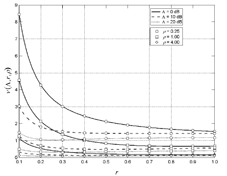
Fig. 2: Shape of $\nu\left({[}\right){\Lambda,r,\rho}]$ versus $r$ for some $\Lambda$’s and $\rho$’s.

Prop. 2

In the asymptotic case where the hypotheses of Prop. 1 hold, the loss $\Psi=u^{*}_{[}{k_{A}}]/u^{*}_{[}{k}]$ of a PRake receiver wrt an ARake receiver in terms of achieved utilities converges a.s. to

$$\Psi\stackrel{{\scriptstyle a.s.}}{{\rightarrow}}\mu\left({[}\right){\Lambda,r}]\cdot\frac{N-\overline{\gamma_{[}]}^{*}\left[(K-1)\mu_{A}\left({[}\right)\Lambda]+\nu_{A}\left({[}\right){\Lambda,\rho}]\right]}{N-\overline{\gamma_{[}]}^{*}\left[(K-1)\mu\left({[}\right){\Lambda,r}]+\nu\left({[}\right){\Lambda,r,\rho}]\right]},$$ (22)

where $u^{*}_{[}{k_{A}}]$ is the utility achieved by an ARake receiver.

The proof of Prop. 2 can be found in [7]. Equation (22) also provides a system design criterion. Given $L$, $N_{c}$, $N_{f}$, $K$ and $\Lambda$, a desired loss $\Psi$ can in fact be achieved using the ratio $r$ obtained by numerically inverting (22).

4.2 Simulation Results

Simulations are performed using the iterative algorithm described in [2]. We assume that each packet contains $100\,\text{b}$ of information and no overhead (i.e., $D=M=100$). We use the efficiency function $f([){\gamma_{[}k]}]=(1-\text{e}^{-\gamma_{[}k]/2})^{M}$ as a reasonable approximation to the PSR. Using $M=100$, $\overline{\gamma_{[}]}^{*}=11.1\,\text{dB}$. We also set $R_{[}]=100\,\text{kb/s}$, $\sigma^{2}=5\times 10^{-16}\,\text{W}$, and $\overline{p}_{[}]=1\,\mu\text{W}$. To model the UWB scenario, the channel gains are assumed as in Sect. 3, with $\sigma^{2}_{{[}}k]=0.3d_{[}k]^{-2}$, where $d_{[}k]$ is the distance between the $k$th user and the base-station. Distances are assumed to be uniformly distributed between $3$ and $20\,\text{m}$.

Fig. 3 shows the probability $P_{o}$ of having at least one user transmitting at the maximum power, i.e., $P_{o}=\operatorname{\mathbb{P}}\{\max_{k}p_{[}k]=\overline{p}_{[}]=1\,\mu\text{W}\}$, as a function of the number of frames $N_{f}$. We consider $10\,000$ realizations of the channel gains, using a network with $K=8$ users, $N_{c}=50$, $L=200$ (thus $\rho=0.25$), and PRake receivers with $L_{P}=20$ coefficients (and thus $r=0.1$). Note that the slope of $P_{o}$ increases as $\Lambda$ increases. This phenomenon is due to reducing the effects of neglected path gains as $\Lambda$ becomes higher, which, given $N_{f}$, results in having more homogeneous effects of neglected gains. Using the parameters above in (21), the minimum value of $N_{f}$ that allows all $K$ users to simultaneously achieve the optimum SINRs is $N_{f}=\{21,9,6\}$ for $\Lambda=\{0\,\text{dB},10\,\text{dB},20\,\text{dB}\}$, respectively. As can be seen, the analytical results closely match with simulations. It is worth emphasize that (21) is valid for both $L$ and $L_{P}$ going to $\infty$, as stated in Prop. 1. In this example, $L_{P}=20$, which does not fulfill this hypothesis. This explains the slight mismatch between theoretical and simulation results, especially for small $\Lambda$’s. However, the authors have found showing numerical results for a feasible system to be more interesting than simulating a network with a very high number of PRake coefficients.

Fig. 4 shows a comparison between analytical and numerical achieved utilities versus the channel gains $h_{[}k]=\left|\left|{\mbox{\boldmath$\alpha$}_{[}k]}\right|\right|^{2}$. The network parameters are $K=8$, $L=200$, $N_{c}=50$, $N_{f}=20$, $\Lambda=10\,\text{dB}$, $\rho=0.25$. The markers correspond to the simulation results given by a single realization of the path gains. Some values of the receiver coefficients are considered. The solid line represents the theoretical achieved utility, computed using (4.1) with $r=1$. The dashed, the dash-dotted and the dotted lines have been obtained by subtracting from (4.1) the loss $\Psi$, computed as in (22). Using the parameters above, $\Psi=\{1.34\,\text{dB},2.94\,\text{dB},8.40\,\text{dB}\}$ for $r=\{0.5,0.3,0.1\}$, respectively. It is worth noting that such lines do not consider the effective values of $h_{[}^{(\text{SP})}k]$, as required in (4.1), since they make use of the asymptotic approximation (22). The analytical results closely match the actual performance of the PRake receivers, especially recalling that the results are not averaged, but only a single random scenario is considered. As before, the larger the number of $L_{P}$ coefficients is, the smaller the difference between theoretical analysis and simulations is.

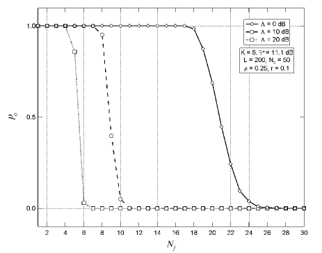
Fig. 3: Probability of having at least one user transmitting at maximum power versus number of frames.

5 Conclusion

In this paper, we have used a large system analysis to study performance of PRake receivers using maximal ratio combining schemes when energy-efficient PC techniques are adopted. We have considered a wireless data network in frequency-selective environments, where the user terminals transmit IR-UWB signals to a common concentration point. Assuming the averaged power delay profile and the amplitude of the path coefficients to be exponentially decaying and Rayleigh-distributed, respectively, we have obtained a general characterization for the terms due to self-interference and multiple access interference. The expressions are dependent only on the network parameters and the number of PRake coefficients. A measure of the loss of PRake receivers with respect to the ARake receiver has then been proposed which is completely independent of the channel realizations. This theoretical approach may also serve as a criterion for network design, since it is completely described by the network parameters.

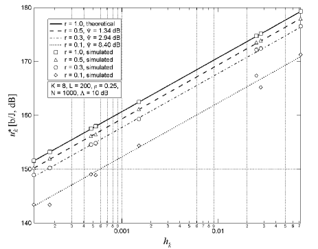
Fig. 4: Achieved utility versus channel gain at the Nash equilibrium for different ratios $r$.

References

- [1] C. U. Saraydar, N. B. Mandayam and D. J. Goodman, “Efficient power control via pricing in wireless data networks,” IEEE Trans. Commun., Vol. 50 (2), pp. 291-303, Feb. 2002.
- [2] G. Bacci, M. Luise, H. V. Poor and A. M. Tulino, “Energy-efficient power control in impulse radio UWB wireless networks,” preprint. [Online]. Available: http://arxiv.org/pdf/cs/0701017.
- [3] J. G. Proakis, Digital Communications, 4th ed. New York, NY, USA: McGraw-Hill, 2001.
- [4] S. Gezici, H. Kobayashi, H. V. Poor and A. F. Molisch, “Performance evaluation of impulse radio UWB systems with pulse-based polarity randomization,” IEEE Trans. Signal Process., Vol. 53 (7), pp. 2537-2549, Jul. 2005.
- [5] U. G. Schuster and H. Bölcskei, “Ultrawideband channel modeling on the basis of information-theoretic criteria,” IEEE Trans. Wireless Commun., 2007, to appear.
- [6] A. F. Molisch, J. R. Foerster and M. Pendergrass, “Channel models for ultrawideband personal area networks,” IEEE Wireless Commun., Vol. 10 (6), pp. 14-21, Dec. 2003.
- [7] G. Bacci, M. Luise and H. V. Poor, “Performance of rake receivers in IR-UWB networks using energy-efficient power control,” preprint. [Online]. Available: http://arxiv.org/pdf/cs/0701034.