Effective Lagrangian for the $\chi^{+}_{j}\chi^{-}_{k}H^{0}_{l}$ interaction in the minimal supersymmetric standard model and neutral Higgs decays

Tarek Ibrahim

Department of Physics, Northeastern University, Boston, MA 02115-5000, USA

and

Department of Physics, Faculty of Science, University of Alexandria, Alexandria, Egypt

Abstract

We extend previous analyses of the supersymmetric loop correction to the neutral Higgs couplings to include the coupling $\chi^{+}_{j}\chi^{-}_{k}H^{0}_{l}$. The analysis completes the previous analyses where similar corrections were computed for the $\bar{\tau}\tau H^{0}_{l}$, $\bar{b}bH^{0}_{l}$, $\bar{c}cH^{0}_{l}$ and for $\bar{t}tH^{0}_{l}$ couplings within the minimal supersymmetric standard model. The effective one loop Lagrangian is then applied to the computation of the neutral Higgs decays. The sizes of the supersymmetric loop corrections of the neutral Higgs decay widths into $\chi^{+}_{i}\chi^{-}_{j}$ ($i=1,2$; $j=1,2$) are investigated and the supersymmetric loop correction is found to be in the range of $7\sim 15\%$ in significant regions of the parameter space. By including the loop corrections of the other decay channels $\bar{b}b$, $\bar{t}t$, $\bar{\tau}\tau$, $\bar{c}c$, and $\chi^{0}_{i}\chi^{0}_{j}$ ($i=1-4$; $j=1-4$), the corrections to branching ratios for $H^{0}_{l}\rightarrow\chi^{+}_{i}\chi^{-}_{j}$ can reach as high as $40\%$. The effects of CP phases on the branching ratio are also investigated.

1 INTRODUCTION

The neutral Higgs couplings to different fields are of great current interest as they enter in a variety of phenomena which are testable in low energy processes [1]. It is known that supersymmetric corrections can affect the neutral Higgs boson decays into $b\bar{b}$, $\tau\bar{\tau}$ and $c\bar{c}$. The decay properties of the lightest Higgs boson in MSSM would be different from those of the Standard Model Higgs boson when these corrections are taken into consideration. Specifically the ratio of the branching ratios to $b\bar{b}$ and $\tau\bar{\tau}$ of the Higgs boson is an important piece of evidence that might distinguish between the lightest MSSM Higgs boson and the Standard Model one at colliders. In MSSM there are also other modes for neutral Higgs decays that do not exist in Standard Model such as charginos and neutralinos.

In this paper we compute the one loop corrected effective Lagrangian for the neutral Higgs and chargino couplings. We then analyze the effects of the loop corrections to the neutral Higgs decays $H^{0}_{l}\rightarrow\chi^{+}_{j}\chi^{-}_{k}$. In the analysis we also include the effect of CP phases arising from the soft SUSY breaking parameters. It is well known that large CP phases can be made compatible [2, 3, 4] with experimental constraints on the electric dipole moments (edms) of the electron [5], of the neutron [6], and of the $Hg^{199}$ [7]. Further, if the phases are large they could affect the Higgs sector physics. It is well known that one loop contributions to the Higgs masses from the stop, sbottom, the chargino and neutralino sectors can lift the lightest Higgs mass above $M_{Z}$. The inclusion of the CP violating phases brings mixings between the CP even and the CP odd Higgs [8, 9, 10, 22, 23, 24]. The CP violating phases modifies the physics of dark matter [11], and of other phenomena [12]. (For a review see Ref.[13].)

The current analysis of $\Delta{\cal{L}}_{H^{0}\chi^{+}\chi^{-}}$ and neutral Higgs decay into charginos is based on the effective Lagrangian method where the couplings of the electroweak eigen states $H^{1}_{1}$ and $H^{2}_{2}$ with charginos are radiatively corrected using the zero external momentum approximation. The same technique has been used in calculating the effective Lagrangian and decays of $H^{0}_{l}$ into quarks and leptons [1, 15, 16]. It has been used also in the analysis of the effective Lagrangian of charged Higgs with quarks [1, 17] and their decays into ${\bar{t}}b$ and $\nu_{\tau}\tau$ [18] and into chargino $+$ neutralino [19]. The neutral Higgs decays into charginos have been investigated before in the CP conserving case [20, 21]. In these analyses, the wave function renormalization and the counter terms for the mass matrix elements are calculated beside the vertex corrections of the mass eigen states $h^{0}$, $H^{0}$ and $A^{0}$ with charginos. In the effective Lagrangian technique with zero external momentum approximation, the radiative corrections of the processes considered here originate only from the vertex contributions. Thus our analysis of the neutral Higgs decays into charginos is a partial one. However, as mentioned before the above analyses were carried out in the CP conserving scenario. As far as we know, the analysis for the neutral Higgs decays into charginos, with one loop corrections, in the CP violating case where the neutral Higgs sector is modified in couplings, spectrum and mixings, does not exist. We evaluate the radiative corrections to the Higgs boson masses and mixngs by using the effective potential approximation. We include the corrections from the top and bottom quarks and squarks [22], from the chargino, the W and the charged Higgs sector [23] and from the neutralino, Z boson, and the neutral Higgs bosons [24]. It is important to notice that the corrections to the Higgs effective potential from the different sectors mentioned above are all one-loop corrections. The corrections of the interaction $\Delta{\cal{L}}_{H^{0}\chi^{+}\chi^{-}}$ to be considered in this work are all one-loop level ones. So the analysis presented here is a consistent one loop study.

The outline of the rest of the paper is as follows: In Sec. 2 we compute the effective Lagrangian for the $\chi^{+}_{j}\chi^{-}_{k}H^{0}_{l}$ interaction. In Sec. 3 we give an analysis of the decay widths of the neutral Higgs bosons into charginos using the effective Lagrangian. In Sec. 4 we give a numerical analysis of the size of the loop effects on the partial decay width and on the branching ratios. Conclusions are given in Sec. 5.

2 LOOP CORRECTIONS TO NEUTRAL HIGGS COUPLINGS

The tree-level Lagrangian for $\chi^{+}_{j}\chi^{-}_{k}H^{0}$ interaction is

$${\cal{L}}=\phi_{jk}\overline{\chi_{j}^{+}}P_{R}\chi^{+}_{k}H^{1}_{1}+\psi_{jk}\overline{\chi_{j}^{+}}P_{R}\chi^{+}_{k}H^{2}_{2}+H.c.,$$ (1)

where $H^{1}_{1}$ and $H^{2}_{2}$ are the neutral states of the two Higgs isodoublets in the minimal supersymmetric standard model (MSSM), i.e.,

$$(H_{1})=\left(\matrix{H_{1}^{1}\cr H_{1}^{2}}\right),~{}~{}(H_{2})=\left(\matrix{H_{2}^{1}\cr H_{2}^{2}}\right)$$ (2)

and the couplings $\phi_{jk}$ and $\psi_{jk}$ are given by

$$\phi_{jk}=-gU_{k2}V_{j1},~{}~{}\psi_{jk}=-gU_{k1}V_{j2}$$ (3)

where U and V diagonalize the chargino mass matrix so that

$$U^{*}M_{\chi^{+}}V^{-1}=diag(m_{\chi^{+}_{1}},m_{\chi^{+}_{2}})$$ (4)

The loop corrections produce shifts in the couplings of Eq. (1) and the effective Lagrangian with loop corrected couplings is given by

$${\cal{L}}_{eff}=(\phi_{jk}+\delta\phi_{jk})\overline{\chi_{j}^{+}}P_{R}\chi^{+}_{k}H^{1}_{1}+\Delta\phi_{jk}\overline{\chi_{j}^{+}}P_{L}\chi^{+}_{k}H^{2}_{2}+$$

$$~{}~{}(\psi_{jk}+\delta\psi_{jk})\overline{\chi_{j}^{+}}P_{R}\chi^{+}_{k}H^{2}_{2}+\Delta\psi_{jk}\overline{\chi_{j}^{+}}P_{L}\chi^{+}_{k}H^{1}_{1}+H.c.$$ (5)

In this work we calculate the loop correction to the $\chi^{+}_{j}\chi^{-}_{k}H^{0}_{l}$ using the zero external momentum approximation.

2.1 Loop analysis of $\delta\phi_{jk}$ and $\Delta\psi_{jk}$

Contributions to $\delta\phi_{jk}$ and $\Delta\psi_{jk}$ arise from the thirteen loop diagram of Fig. 1. We note that the contribution from diagrams which have $H^{+}W^{+}H^{0}$and $H^{0}Z^{0}H^{0}$ vertices do not contribute in the effective Lagrangian with zero external momentum approximation since these vertices are proportional to the external momentum. We discuss now in detail the contribution of each of these diagrams in Fig. 1. We begin with the loop diagram of Fig. 1i(a) which contributes to $\delta\phi_{jk}$ and $\Delta\psi_{jk}$.

We calculate the corrections of the amplitude from Fig. 1i(a)

$$\delta M=i\delta\phi_{jk}\bar{u}_{j}P_{R}v_{k}+i\Delta\psi_{jk}\bar{u}_{j}P_{L}v_{k}$$ (6)

The idea is to extract, from the amplitude correction, the expressions for $\delta\phi_{jk}$ and $\Delta\psi_{jk}$ from those parts that are proportional to $\bar{u}_{j}P_{R}v_{k}$ and $\bar{u}_{j}P_{L}v_{k}$ respectively. For this purpose we need $\tilde{b}\tilde{b}H^{1}_{1}$ interaction which is given by

$${\cal{L}}_{\tilde{b}\tilde{b}H^{1}_{1}}=H_{il}\tilde{b}^{*}_{i}\tilde{b}^{*}_{l}H^{1}_{1}+H.c.$$ (7)

where $H_{il}$ is given by

$$H_{il}=-\frac{gM_{Z}}{\sqrt{2}\cos\theta_{W}}((-\frac{1}{2}+\frac{1}{3}\sin^{2}\theta_{W})D_{b1i}^{*}D_{b1l}-\frac{1}{3}\sin^{2}\theta_{W}D_{b2i}^{*}D_{b2l})\cos\beta$$

$$-\frac{gm^{2}_{b}}{\sqrt{2}m_{W}\cos\beta}(D_{b1i}^{*}D_{b1l}+D_{b2i}^{*}D_{b2l})-\frac{gm_{b}A_{b}}{\sqrt{2}m_{W}\cos\beta}D_{b2i}^{*}D_{b1l}$$ (8)

The matrix elements $D_{q}$ are defined as

$$D^{+}_{q}M^{2}_{\tilde{q}}D_{q}=diag(m^{2}_{\tilde{q1}},m^{2}_{\tilde{q2}})$$ (9)

We need also the $\bar{t}\chi^{+}\tilde{b}$ interaction which is given by

$${\cal{L}}_{\bar{t}\chi^{+}\tilde{b}}=-g\bar{\chi^{+}_{k}}[(U^{*}_{k1}D^{*}_{b_{1i}}-\kappa_{b}U^{*}_{k2}D^{*}_{b_{2i}})P_{L}$$

$$-\kappa_{t}V_{k2}D^{*}_{b_{1i}}P_{R}]t\tilde{b}^{*}_{i}+H.c$$ (10)

where $\kappa_{t,b}$ are given by

$$\kappa_{t}=\frac{m_{t}}{\sqrt{2}m_{W}\sin\beta}$$

$$~{}\kappa_{b}=\frac{m_{b}}{\sqrt{2}m_{W}\cos\beta}$$ (11)

For external momenta $s$, $q$ and $q-s$ the amplitude correction from loop 1i(a) is given by

$$\delta M=-g^{2}H_{il}\bar{u}(q-s)[C_{L_{jl}}P_{L}+C_{R_{jl}}P_{R}]$$

$$\int\frac{d^{4}\ell}{(2\pi)^{4}}[(\not\!s+\not\!\ell)+m_{t}][C^{*}_{L_{ki}}P_{R}+C^{*}_{R_{ki}}P_{L}]v(s)$$

$$\times\frac{1}{((s+\ell)^{2}-m^{2}_{t}+i\epsilon)(\ell^{2}-m^{2}_{\tilde{b_{l}}}+i\epsilon)((\ell+q)^{2}-m^{2}_{\tilde{b_{i}}}+i\epsilon)}$$ (12)

where $C_{L_{jl}}$ and $C_{R_{jl}}$ are given by

$$C_{L_{jl}}=U^{*}_{j1}D^{*}_{b_{1l}}-\kappa_{b}U^{*}_{j2}D^{*}_{b_{2l}}$$

$$C_{R_{jl}}=-\kappa_{t}V_{j2}D^{*}_{b_{1l}}$$ (13)

The part in the numerator

$$[C_{L_{jl}}P_{L}+C_{R_{jl}}P_{R}][(\not\!s+\not\!\ell)+m_{t}]$$

$$(C^{*}_{L_{ki}}P_{R}+C^{*}_{R_{ki}}P_{L})$$ (14)

could be written as

$$[C_{L_{jl}}C^{*}_{L_{ki}}P_{L}+C_{R_{jl}}C^{*}_{R_{ki}}P_{R}](\not\!s+\not\!\ell)$$

$$+m_{t}[C_{R_{jl}}C^{*}_{L_{ki}}P_{R}+C_{L_{jl}}C^{*}_{R_{ki}}P_{L}]$$ (15)

by using the facts that $\gamma^{\mu}P_{L}=P_{R}\gamma^{\mu}$, $P_{L}P_{R}=0$, $P^{2}_{L}=P_{L}$ and $P^{2}_{R}=P_{R}$. The first term in Eq. (15) does not contribute to $\delta\phi_{jk}$ or $\Delta\psi_{jk}$ since it does not have the same Lorentz structure. The second term of Eq. (15) contributes the part of $m_{t}C_{R_{jl}}C^{*}_{L_{ki}}$ to $\delta\phi_{jk}$ and $m_{t}C_{L_{jl}}C^{*}_{R_{ki}}$ to $\Delta\psi_{jk}$. Thus the loop corrections $\delta\phi_{jk}$ and $\Delta\psi_{jk}$ read

$$i\delta\phi_{jk}=-g^{2}H_{il}m_{t}C_{R_{jl}}C^{*}_{L_{ki}}J$$

$$i\Delta\psi_{jk}=-g^{2}H_{il}m_{t}C_{L_{jl}}C^{*}_{R_{ki}}J$$

where

$$J=\int\frac{d^{4}\ell}{(2\pi)^{4}}\frac{1}{((s+\ell)^{2}-m^{2}_{t}+i\epsilon)(\ell^{2}-m^{2}_{\tilde{b_{l}}}+i\epsilon)((\ell+q)^{2}-m^{2}_{\tilde{b_{i}}}+i\epsilon)}$$ (17)

Now for zero external momentum approximation we set $s=q=0$, and the integral would read

$$\int\frac{d^{4}\ell}{(2\pi)^{4}}\frac{1}{(\ell^{2}-m^{2}_{t}+i\epsilon)(\ell^{2}-m^{2}_{\tilde{b_{l}}}+i\epsilon)(\ell^{2}-m^{2}_{\tilde{b_{i}}}+i\epsilon)}$$ (18)

A detailed calculation of this integral is given in the appendix.

Using the above one finds for $\delta\phi_{jk}$ the contribution:

$$\delta\phi^{(1)}_{jk}=\kappa_{t}\frac{g^{2}m_{t}}{16\pi^{2}}\sum_{i=1}^{2}\sum_{l=1}^{2}H_{il}V_{j2}D^{*}_{b_{1l}}(U_{k1}D_{b_{1i}}-\kappa_{b}U_{k2}D_{b_{2i}})f(m^{2}_{t},m^{2}_{\tilde{b}_{l}},m^{2}_{\tilde{b}_{i}})$$ (19)

where

$$f(x,y,z)=\frac{1}{(x-y)(x-z)(z-y)}\times(zxln\frac{z}{x}+xyln\frac{x}{y}+yzln\frac{y}{z}),$$ (20)

and

$$f(x,y,y)=\frac{1}{(y-x)^{2}}\times(xln\frac{y}{x}+x-y)$$ (21)

Similarly one finds for the correction $\Delta\psi_{jk}$ from the same loop the following contribution

$$\Delta\psi^{(1)}_{jk}=\kappa_{t}\frac{g^{2}m_{t}}{16\pi^{2}}\sum_{i=1}^{2}\sum_{l=1}^{2}H_{il}V^{*}_{k2}D_{b_{1i}}(U^{*}_{j1}D^{*}_{b_{1l}}-\kappa_{b}U^{*}_{j2}D^{*}_{b_{2l}})f(m^{2}_{t},m^{2}_{\tilde{b}_{l}},m^{2}_{\tilde{b}_{i}})$$ (22)

Next for the loop Fig. 1ii(a) we find

$$\delta\phi^{(2)}_{jk}=0$$

$$~{}\Delta\psi^{(2)}_{jk}=0$$ (23)

For the loop of Fig. 1i(b) we find

$$\delta\phi^{(3)}_{jk}=\kappa_{b}\frac{g^{2}m_{b}}{16\pi^{2}}\sum_{i=1}^{2}\sum_{l=1}^{2}F_{li}U_{k2}D^{*}_{t_{1i}}(V_{j1}D_{t_{1l}}-\kappa_{t}V_{j2}D_{t_{2l}})f(m^{2}_{b},m^{2}_{\tilde{t}_{i}},m^{2}_{\tilde{t}_{l}})$$

$$\Delta\psi^{(3)}_{jk}=\kappa_{b}\frac{g^{2}m_{b}}{16\pi^{2}}\sum_{i=1}^{2}\sum_{l=1}^{2}F_{li}U^{*}_{j2}D_{t_{1l}}(V^{*}_{k1}D^{*}_{t_{1i}}-\kappa_{t}V^{*}_{k2}D^{*}_{t_{2i}})f(m^{2}_{b},m^{2}_{\tilde{t}_{i}},m^{2}_{\tilde{t}_{l}})$$ (24)

where $F_{li}$ is given by

$$F_{li}=-\frac{gM_{Z}}{\sqrt{2}\cos\theta_{W}}((\frac{1}{2}-\frac{2}{3}\sin^{2}\theta_{W})D_{t1l}^{*}D_{t1i}+\frac{2}{3}\sin^{2}\theta_{W}D_{t2l}^{*}D_{t2i})\cos\beta$$

$$+\frac{gm_{t}\mu}{\sqrt{2}m_{W}\sin\beta}D_{t1l}^{*}D_{t2i}$$ (25)

For the loop of Fig. 1ii(b) we find

$$\delta\phi^{(4)}_{jk}=0$$

$$\Delta\psi^{(4)}_{jk}=-\kappa_{b}\frac{g^{2}m^{2}_{b}}{16\pi^{2}}h_{b}\sum_{i=1}^{2}U^{*}_{j2}D_{t_{1i}}(V^{*}_{k1}D^{*}_{t_{1i}}-\kappa_{t}V^{*}_{k2}D^{*}_{t_{2i}})f(m^{2}_{b},m^{2}_{b},m^{2}_{\tilde{t}_{i}})$$ (26)

For loop of Fig. 1ii(c) we find

$$\delta\phi^{(5)}_{jk}=2g\sum_{i=1}^{4}\sum_{l=1}^{4}Q^{{}^{\prime}}_{il}\epsilon^{{}^{\prime}}_{ik}\sin\beta\epsilon^{*}_{lj}\cos\beta$$

$$\frac{m_{\chi^{0}_{i}}m_{\chi^{0}_{l}}}{16\pi^{2}}f(m^{2}_{\chi^{0}_{i}},m^{2}_{\chi^{0}_{l}},m^{2}_{H^{+}})$$

$$\Delta\psi^{(5)}_{jk}=0$$ (27)

where $\epsilon^{{}^{\prime}}$ and $\epsilon$ are given by

$$\epsilon_{ji}=-gX_{4j}V_{i1}^{*}-\frac{g}{\sqrt{2}}X_{2j}V_{i2}^{*}-\frac{g}{\sqrt{2}}\tan\theta_{W}X_{1j}V_{i2}^{*}$$

$$~{}\epsilon^{{}^{\prime}}_{ji}=-gX_{3j}^{*}U_{i1}+\frac{g}{\sqrt{2}}X_{2j}^{*}U_{i2}+\frac{g}{\sqrt{2}}\tan\theta_{W}X_{1j}^{*}U_{i2}$$ (28)

The parameters $Q^{{}^{\prime}}_{ij}$ are defined as:

$$Q^{{}^{\prime}}_{ij}=\frac{1}{\sqrt{2}}[X^{*}_{3i}(X^{*}_{2j}-\tan\theta_{W}X^{*}_{1j})]$$ (29)

The matrix elements $X$ are defined as

$$X^{T}M_{\chi^{0}}X=diag(m_{\chi^{0}_{1}},m_{\chi^{0}_{2}},m_{\chi^{0}_{3}},m_{\chi^{0}_{4}})$$ (30)

For loop of Fig. 1i(c) we find

$$\delta\phi^{(6)}_{jk}=\frac{gm_{W}\cos\beta}{2\sqrt{2}}[1+2\sin^{2}\beta-\cos 2\beta\tan^{2}\theta_{W}]\sum_{i=1}^{4}$$

$$\epsilon^{{}^{\prime}}_{ik}\sin\beta\epsilon^{*}_{ij}\cos\beta$$

$$\frac{m_{\chi^{0}_{i}}}{16\pi^{2}}f(m^{2}_{\chi^{0}_{i}},m^{2}_{H^{+}},m^{2}_{H^{+}})$$

$$\Delta\psi^{(6)}_{jk}=\frac{gm_{W}\cos\beta}{2\sqrt{2}}[1+2\sin^{2}\beta-\cos 2\beta\tan^{2}\theta_{W}]\sum_{i=1}^{4}$$

$$\epsilon_{ik}\cos\beta\epsilon^{{}^{\prime}*}_{ij}\sin\beta$$

$$\frac{m_{\chi^{0}_{i}}}{16\pi^{2}}f(m^{2}_{\chi^{0}_{i}},m^{2}_{H^{+}},m^{2}_{H^{+}})$$ (31)

For loop of Fig. 1i(d) we find

$$\delta\phi^{(7)}_{jk}=g^{3}\frac{m_{Z}\cos\beta}{8\sqrt{2}\cos\theta_{W}}\sum_{l=1}^{3}\sum_{m=1}^{3}\sum_{i=1}^{2}((Y_{m1}-iY_{m3}\sin\beta)(3Y_{l1}+iY_{l3}\sin\beta)$$

$$-2(Y_{m2}-iY_{m3}\cos\beta)(Y_{l2}+iY_{l3}\cos\beta)-4Y_{m2}(Y_{l1}-iY_{l3}\sin\beta)\tan\beta)$$

$$(Q_{ki}(Y_{l1}+iY_{l3}\sin\beta)+S_{ki}(Y_{l2}+iY_{l3}\cos\beta))$$

$$(Q_{ij}(Y_{m1}+iY_{m3}\sin\beta)+S_{ij}(Y_{m2}+iY_{m3}\cos\beta))$$

$$\frac{m_{\chi^{+}_{i}}}{16\pi^{2}}f(m^{2}_{\chi^{+}_{i}},m^{2}_{H^{0}_{m}},m^{2}_{H^{0}_{l}})$$

$$\Delta\psi^{(7)}_{jk}=g^{3}\frac{m_{Z}\cos\beta}{8\sqrt{2}\cos\theta_{W}}\sum_{l=1}^{3}\sum_{m=1}^{3}\sum_{i=1}^{2}((Y_{m1}-iY_{m3}\sin\beta)(3Y_{l1}+iY_{l3}\sin\beta)$$

$$-2(Y_{m2}-iY_{m3}\cos\beta)(Y_{l2}+iY_{l3}\cos\beta)-4Y_{m2}(Y_{l1}-iY_{l3}\sin\beta)\tan\beta)$$

$$(Q^{*}_{ik}(Y_{l1}-iY_{l3}\sin\beta)+S^{*}_{ik}(Y_{l2}-iY_{l3}\cos\beta))$$

$$(Q^{*}_{ji}(Y_{m1}-iY_{m3}\sin\beta)+S^{*}_{ji}(Y_{m2}-iY_{m3}\cos\beta))$$

$$\frac{m_{\chi^{+}_{i}}}{16\pi^{2}}f(m^{2}_{\chi^{+}_{i}},m^{2}_{H^{0}_{m}},m^{2}_{H^{0}_{l}})$$ (32)

where $Q_{ji}=-\frac{1}{\sqrt{2}g}\phi_{ij}$ and $S_{ji}=\frac{1}{\sqrt{2}g}\psi_{ij}$, and the matrix elements $Y$ are defined as $YM^{2}_{Higgs}Y^{T}=diag(m^{2}_{H^{0}_{1}},m^{2}_{H^{0}_{2}},m^{2}_{H^{0}_{3}})$.

For loop of Fig. 1ii(d) we find

$$\delta\phi^{(8)}_{jk}=-g^{2}\sum_{m=1}^{3}\sum_{i=1}^{2}\sum_{l=1}^{2}\phi_{li}$$

$$(Q_{li}(Y_{m1}+iY_{m3}\sin\beta)+S_{lj}(Y_{m2}+iY_{m3}\cos\beta))(Q_{ki}(Y_{m1}+iY_{m3}\sin\beta)$$

$$+S_{ki}(Y_{m2}+iY_{m3}\cos\beta))\frac{m_{\chi^{+}_{i}}m_{\chi^{+}_{l}}}{16\pi^{2}}f(m^{2}_{\chi^{+}_{i}},m^{2}_{H^{0}_{m}},m^{2}_{\chi^{+}_{l}})$$

$$\Delta\psi^{(8)}_{jk}=0$$ (33)

For loop of Fig. 1ii(e) we find

$$\delta\phi^{(9)}_{jk}=0$$

$$~{}\Delta\psi^{(9)}_{jk}=\frac{4g^{2}}{\cos^{2}\theta_{W}}\sum_{l=1}^{2}\sum_{i=1}^{2}\phi_{li}R^{\prime}_{jl}L^{\prime}_{ik}\frac{m_{\chi^{+}_{i}}m_{\chi^{+}_{l}}}{16\pi^{2}}f(m^{2}_{\chi^{+}_{i}},m^{2}_{Z_{0}},m^{2}_{\chi^{+}_{l}})$$ (34)

The parameters $L^{\prime}$ and $R^{\prime}$ are defined by

$$L_{ij}^{{}^{\prime}}=-V_{i1}V^{*}_{j1}-\frac{1}{2}V_{i2}V^{*}_{j2}+\delta_{ij}\sin^{2}\theta_{W}$$

$$~{}R_{ij}^{{}^{\prime}}=-U^{*}_{i1}U_{j1}-\frac{1}{2}U^{*}_{i2}U_{j2}+\delta_{ij}\sin^{2}\theta_{W}$$ (35)

For loop of Fig. 1i(e) we find

$$\delta\phi^{(10)}_{jk}=-\frac{\sqrt{2}g^{3}m_{Z}\cos\beta}{\cos^{3}\theta_{W}}\sum_{i=1}^{2}L^{\prime}_{ji}R^{\prime}_{ik}\frac{m_{\chi^{+}_{i}}}{16\pi^{2}}f(m^{2}_{\chi^{+}_{i}},m^{2}_{Z_{0}},m^{2}_{Z_{0}})$$

$$~{}\Delta\psi^{(10)}_{jk}=-\frac{\sqrt{2}g^{3}m_{Z}\cos\beta}{\cos^{3}\theta_{W}}\sum_{i=1}^{2}R^{\prime}_{ji}L^{\prime}_{ik}\frac{m_{\chi^{+}_{i}}}{16\pi^{2}}f(m^{2}_{\chi^{+}_{i}},m^{2}_{Z_{0}},m^{2}_{Z_{0}})$$ (36)

For loop of Fig. 1ii(f) we find

$$\delta\phi^{(11)}_{jk}=0$$

$$~{}\Delta\psi^{(11)}_{jk}=-4\sqrt{2}g^{3}\sum_{i=1}^{4}\sum_{l=1}^{4}Q"_{il}R^{*}_{lj}L_{ik}\frac{m_{\chi^{0}_{i}}m_{\chi^{0}_{l}}}{16\pi^{2}}f(m^{2}_{\chi^{0}_{i}},m^{2}_{W^{+}},m^{2}_{\chi^{0}_{l}})$$ (37)

where $L$, $R$ and $Q"$ are defined as

$$L_{ij}=-\frac{1}{\sqrt{2}}X^{*}_{4i}V^{*}_{j2}+X^{*}_{2i}V^{*}_{j1}$$

$$~{}R_{ij}=\frac{1}{\sqrt{2}}X_{3i}U_{j2}+X_{2i}U_{j1}$$

$$~{}gQ^{"}=\frac{1}{2}(X^{*}_{3i}(gX^{*}_{2j}-g^{\prime}X^{*}_{1j})+(i\leftrightarrow j))$$ (38)

For loop of Fig. 1i(f) we find

$$\delta\phi^{(12)}_{jk}=-\frac{4g^{3}m_{W}\cos\beta}{\sqrt{2}}\sum_{i=1}^{4}L^{*}_{ij}R_{ik}\frac{m_{\chi^{0}_{i}}}{16\pi^{2}}f(m^{2}_{\chi^{0}_{i}},m^{2}_{W^{+}},m^{2}_{W^{+}})$$

$$~{}\Delta\psi^{(12)}_{jk}=-\frac{4g^{3}m_{W}\cos\beta}{\sqrt{2}}\sum_{i=1}^{4}R^{*}_{ij}L_{ik}\frac{m_{\chi^{0}_{i}}}{16\pi^{2}}f(m^{2}_{\chi^{0}_{i}},m^{2}_{W^{+}},m^{2}_{W^{+}})$$ (39)

For loop of Fig. 1ii(g) we find

$$\delta\phi^{(13)}_{jk}=0$$

$$~{}\Delta\psi^{(13)}_{jk}=-g^{2}h_{\tau}\kappa_{\tau}U^{*}_{j2}V^{*}_{k1}\frac{m^{2}_{\tau}}{16\pi^{2}}f(m^{2}_{\tau},m^{2}_{\tau},m^{2}_{\nu_{\tau}})$$ (40)

where

$$\kappa_{\tau}=\frac{m_{\tau}}{\sqrt{2}m_{W}\cos\beta}$$ (41)

The loop corrections for $\delta\phi_{jk}$ and $\Delta\psi_{jk}$ are given by

$$\delta\phi_{jk}=\sum_{n=1}^{13}\delta\phi^{(n)}_{jk}$$

$$~{}\Delta\psi_{jk}=\sum_{n=1}^{13}\Delta\psi^{(n)}_{jk}$$ (42)

2.2 Loop analysis of $\Delta\phi_{jk}$ and $\delta\psi_{jk}$

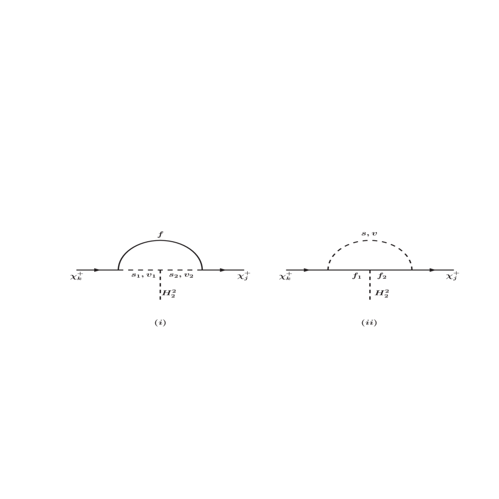
Figure 2: Set of diagrams contributing to radiative corrections $\Delta\phi_{jk}$ and $\delta\psi_{jk}$. (i): (a) $s_{1}=\tilde{b}_{i}^{*}$, $s_{2}=\tilde{b}_{l}^{*}$, $f=t$; (b) $s_{1}=\tilde{t}_{i}$, $s_{2}=\tilde{t}_{l}$, $f=\bar{b}$; (c) $s_{1}=H^{+}$, $s_{2}=H^{+}$, $f=\chi^{0}_{i}$; (d) $s_{1}=H^{0}_{l}$, $s_{2}=H^{0}_{m}$, $f=\chi^{+}_{i}$; (e) $v_{1}=Z^{0}$, $v_{2}=Z^{0}$, $f=\chi^{+}_{i}$; (f) $v_{1}=W^{+}$, $v_{2}=W^{+}$, $f=\chi^{0}_{i}$. (ii): (a) $f_{1}=t$, $f_{2}=t$, $s=\tilde{b}_{i}^{*}$; (b) $f_{1}=\bar{b}$, $f_{2}=\bar{b}$, $s=\tilde{t}_{i}$; (c)$f_{1}=\chi^{0}_{i}$, $f_{2}=\chi^{0}_{l}$, $s=H^{+}$; (d) $f_{1}=\chi^{+}_{i}$, $f_{2}=\chi^{+}_{l}$, $s=H^{0}_{m}$; (e) $f_{1}=\chi^{+}_{i}$, $f_{2}=\chi^{+}_{l}$, $v=Z^{0}$; (f) $f_{1}=\chi^{0}_{i}$, $f_{2}=\chi^{0}_{l}$, $v=W$; (g) $f_{1}=\tau^{+}$, $f_{2}=\tau^{+}$, $s=\tilde{\nu}_{\tau}$.

We do the same analysis of Fig. 2 as for Fig. 1. We write down here the final results for both corrections from the thirteen loops together. The corrections are written in the same order of the loops in Fig. 2.

$$\Delta\phi_{jk}=\kappa_{t}\frac{g^{2}m_{t}}{16\pi^{2}}\sum_{i=1}^{2}\sum_{l=1}^{2}G_{il}V^{*}_{k2}D_{b_{1i}}(U^{*}_{j1}D^{*}_{b_{1l}}-\kappa_{b}U^{*}_{j2}D^{*}_{b_{2l}})f(m^{2}_{t},m^{2}_{\tilde{b}_{l}},m^{2}_{\tilde{b}_{i}})$$

$$-\kappa_{t}h_{t}\frac{g^{2}m^{2}_{t}}{16\pi^{2}}\sum_{i=1}^{2}V^{*}_{k2}D_{b_{1i}}(U^{*}_{j1}D^{*}_{b_{1i}}-\kappa_{b}U^{*}_{j2}D^{*}_{b_{2i}})f(m^{2}_{t},m^{2}_{t},m^{2}_{\tilde{b}_{i}})$$

$$+\kappa_{b}\frac{g^{2}m_{b}}{16\pi^{2}}\sum_{i=1}^{2}\sum_{l=1}^{2}E_{li}U^{*}_{j2}D_{t_{1l}}(V^{*}_{k1}D^{*}_{t_{1i}}-\kappa_{t}V^{*}_{k2}D^{*}_{t_{2i}})f(m^{2}_{b},m^{2}_{\tilde{t}_{i}},m^{2}_{\tilde{t}_{l}})$$

$$+0$$

$$+0$$

$$+\frac{gm_{W}\sin\beta}{2\sqrt{2}}[1+2\cos^{2}\beta+\cos 2\beta\tan^{2}\theta_{W}]\sum_{i=1}^{4}$$

$$\epsilon_{ik}\cos\beta\epsilon^{{}^{\prime}*}_{ij}\sin\beta$$

$$\frac{m_{\chi^{0}_{i}}}{16\pi^{2}}f(m^{2}_{\chi^{0}_{i}},m^{2}_{H^{+}},m^{2}_{H^{+}})$$

$$+g^{3}\frac{m_{Z}\cos\beta}{8\sqrt{2}\cos\theta_{W}}\sum_{l=1}^{3}\sum_{m=1}^{3}\sum_{i=1}^{2}(\tan\beta(Y_{l2}-iY_{l3}\cos\beta)(3Y_{m2}+iY_{m3}\cos\beta)$$

$$-4Y_{l1}(Y_{m2}-iY_{m3}\cos\beta)-2\tan\beta(Y_{m1}-iY_{m3}\sin\beta)(Y_{l1}+iY_{l3}\sin\beta))$$

$$(Q^{*}_{ik}(Y_{l1}-iY_{l3}\sin\beta)+S^{*}_{ik}(Y_{l2}-iY_{l3}\cos\beta))$$

$$(Q^{*}_{ji}(Y_{m1}-iY_{m3}\sin\beta)+S^{*}_{ji}(Y_{m2}-iY_{m3}\cos\beta))$$

$$\frac{m_{\chi^{+}_{i}}}{16\pi^{2}}f(m^{2}_{\chi^{+}_{i}},m^{2}_{H^{0}_{m}},m^{2}_{H^{0}_{l}})$$

$$+0$$

$$+\frac{4g^{2}}{\cos^{2}\theta_{W}}\sum_{l=1}^{2}\sum_{i=1}^{2}\psi_{li}R^{\prime}_{jl}L^{\prime}_{ik}\frac{m_{\chi^{+}_{i}}m_{\chi^{+}_{l}}}{16\pi^{2}}f(m^{2}_{\chi^{+}_{i}},m^{2}_{Z_{0}},m^{2}_{\chi^{+}_{l}})$$

$$-\frac{\sqrt{2}g^{3}m_{Z}\sin\beta}{\cos^{3}\theta_{W}}\sum_{i=1}^{2}R^{\prime}_{ji}L^{\prime}_{ik}\frac{m_{\chi^{+}_{i}}}{16\pi^{2}}f(m^{2}_{\chi^{+}_{i}},m^{2}_{Z_{0}},m^{2}_{Z_{0}})$$

$$-4\sqrt{2}g^{3}\sum_{i=1}^{4}\sum_{l=1}^{4}S"_{il}R^{*}_{lj}L_{ik}\frac{m_{\chi^{0}_{i}}m_{\chi^{0}_{l}}}{16\pi^{2}}f(m^{2}_{\chi^{0}_{i}},m^{2}_{W^{+}},m^{2}_{\chi^{0}_{l}})$$

$$-\frac{4g^{3}m_{W}\sin\beta}{\sqrt{2}}\sum_{i=1}^{4}R^{*}_{ij}L_{ik}\frac{m_{\chi^{0}_{i}}}{16\pi^{2}}f(m^{2}_{\chi^{0}_{i}},m^{2}_{W^{+}},m^{2}_{W^{+}})$$

$$+0$$ (43)

where $G$ and $E$ are given by

$$G_{ij}=\frac{gM_{Z}}{\sqrt{2}\cos\theta_{W}}((-\frac{1}{2}+\frac{1}{3}\sin^{2}\theta_{W})D_{b1i}^{*}D_{b1j}-\frac{1}{3}\sin^{2}\theta_{W}D_{b2i}^{*}D_{b2j})\sin\beta$$

$$+\frac{gm_{b}\mu}{\sqrt{2}m_{W}\cos\beta}D_{b1i}^{*}D_{b2j}$$

$$E_{ij}=\frac{gM_{Z}}{\sqrt{2}\cos\theta_{W}}((\frac{1}{2}-\frac{2}{3}\sin^{2}\theta_{W})D_{t1i}^{*}D_{t1j}+\frac{2}{3}\sin^{2}\theta_{W}D_{t2i}^{*}D_{t2j})\sin\beta$$

$$-\frac{gm^{2}_{t}}{\sqrt{2}m_{W}\sin\beta}(D_{t1i}^{*}D_{t1j}+D_{t2i}^{*}D_{t2j})-\frac{gm_{t}A_{t}}{\sqrt{2}m_{W}\sin\beta}D_{t2i}^{*}D_{t2j}$$ (44)

and $S"$ is given by

$$S^{"}_{li}=-\frac{1}{\sin\beta}(\frac{M_{l}}{2m_{W}}\delta_{li}-Q^{"}_{li}\cos\beta-R^{"}_{li})$$

$$R^{"}_{li}=\frac{1}{2m_{W}}(\tilde{m_{1}}^{*}X_{1l}^{*}X_{1i}^{*}+\tilde{m_{2}}^{*}X_{2l}^{*}X_{2i}^{*}-\mu^{*}(X_{3l}^{*}X_{4i}^{*}+X_{4l}^{*}X_{3i}^{*}))$$ (45)

The corrections $\delta\psi_{jk}$ are given by

$$\delta\psi_{jk}=\kappa_{t}\frac{g^{2}m_{t}}{16\pi^{2}}\sum_{i=1}^{2}\sum_{l=1}^{2}G_{il}V_{j2}D^{*}_{b_{1l}}(U_{k1}D_{b_{1i}}-\kappa_{b}U_{k2}D_{b_{2i}})f(m^{2}_{t},m^{2}_{\tilde{b}_{l}},m^{2}_{\tilde{b}_{i}})$$

$$+0$$

$$+\kappa_{b}\frac{g^{2}m_{b}}{16\pi^{2}}\sum_{i=1}^{2}\sum_{l=1}^{2}E_{li}U_{k2}D^{*}_{t_{1i}}(V_{j1}D_{t_{1l}}-\kappa_{t}V_{j2}D_{t_{2l}})f(m^{2}_{b},m^{2}_{\tilde{t}_{i}},m^{2}_{\tilde{t}_{l}})$$

$$+0$$

$$-2g\sum_{i=1}^{4}\sum_{l=1}^{4}S^{{}^{\prime}}_{il}\epsilon^{{}^{\prime}}_{ik}\sin\beta\epsilon^{*}_{lj}\cos\beta$$

$$\frac{m_{\chi^{0}_{i}}m_{\chi^{0}_{l}}}{16\pi^{2}}f(m^{2}_{\chi^{0}_{i}},m^{2}_{\chi^{0}_{l}},m^{2}_{H^{+}})$$

$$+\frac{gm_{W}\sin\beta}{2\sqrt{2}}[1+2\cos^{2}\beta+\cos 2\beta\tan^{2}\theta_{W}]\sum_{i=1}^{4}$$

$$\epsilon^{{}^{\prime}}_{ik}\sin\beta\epsilon^{*}_{ij}\cos\beta$$

$$\frac{m_{\chi^{0}_{i}}}{16\pi^{2}}f(m^{2}_{\chi^{0}_{i}},m^{2}_{H^{+}},m^{2}_{H^{+}})$$

$$+g^{3}\frac{m_{Z}\cos\beta}{8\sqrt{2}\cos\theta_{W}}\sum_{l=1}^{3}\sum_{m=1}^{3}\sum_{i=1}^{2}(\tan\beta(Y_{l2}-iY_{l3}\cos\beta)(3Y_{m2}+iY_{m3}\cos\beta)$$

$$-4Y_{l1}(Y_{m2}-iY_{m3}\cos\beta)-2\tan\beta(Y_{m1}-iY_{m3}\sin\beta)(Y_{l1}+iY_{l3}\sin\beta))$$

$$(Q_{ki}(Y_{l1}+iY_{l3}\sin\beta)+S_{ki}(Y_{l2}+iY_{l3}\cos\beta))$$

$$(Q_{ij}(Y_{m1}+iY_{m3}\sin\beta)+S_{ij}(Y_{m2}+iY_{m3}\cos\beta))$$

$$\frac{m_{\chi^{+}_{i}}}{16\pi^{2}}f(m^{2}_{\chi^{+}_{i}},m^{2}_{H^{0}_{m}},m^{2}_{H^{0}_{l}})$$

$$-g^{2}\sum_{m=1}^{3}\sum_{i=1}^{2}\sum_{l=1}^{2}\psi_{li}$$

$$(Q_{lj}(Y_{m1}+iY_{m3}\sin\beta)+S_{lj}(Y_{m2}+iY_{m3}\cos\beta))(Q_{ki}(Y_{m1}+iY_{m3}\sin\beta)$$

$$+S_{ki}(Y_{m2}+iY_{m3}\cos\beta))\frac{m_{\chi^{+}_{i}}m_{\chi^{+}_{l}}}{16\pi^{2}}f(m^{2}_{\chi^{+}_{i}},m^{2}_{H^{0}_{m}},m^{2}_{\chi^{+}_{l}})$$

$$+0$$

$$-\frac{\sqrt{2}g^{3}m_{Z}\sin\beta}{\cos^{3}\theta_{W}}\sum_{i=1}^{2}L^{\prime}_{ji}R^{\prime}_{ik}\frac{m_{\chi^{+}_{i}}}{16\pi^{2}}f(m^{2}_{\chi^{+}_{i}},m^{2}_{Z_{0}},m^{2}_{Z_{0}})$$

$$+0$$

$$-\frac{4g^{3}m_{W}\sin\beta}{\sqrt{2}}\sum_{i=1}^{4}L^{*}_{ij}R_{ik}\frac{m_{\chi^{0}_{i}}}{16\pi^{2}}f(m^{2}_{\chi^{0}_{i}},m^{2}_{W^{+}},m^{2}_{W^{+}})$$

$$+0$$ (46)

where $S^{\prime}$ is given by

$$S^{{}^{\prime}}_{ij}=\frac{1}{\sqrt{2}}[X^{*}_{4j}(X^{*}_{2i}-\tan\theta_{W}X^{*}_{1i})]$$ (47)

3 Neutral Higgs decays including loop effects

We summarize now the result of the analysis. Thus ${\cal{L}}_{eff}$ of $Eq.(5)$ may be written as follows

$${\cal{L}}_{eff}=H^{0}_{l}\overline{\chi^{+}_{j}}(\alpha^{lS}_{jk}+\gamma_{5}\alpha^{lP}_{jk})\chi^{+}_{k}+H.c$$ (48)

where

$$\alpha^{lS}_{jk}=\frac{1}{2\sqrt{2}}((Y_{l1}+iY_{l3}\sin\beta)(\phi_{jk}+\delta\phi_{jk}+\Delta\psi_{jk})+(Y_{l2}+iY_{l3}\cos\beta)(\psi_{jk}+\delta\psi_{jk}+\Delta\phi_{jk}))$$ (49)

and where

$$\alpha^{lP}_{jk}=\frac{1}{2\sqrt{2}}((Y_{l1}+iY_{l3}\sin\beta)(\phi_{jk}+\delta\phi_{jk}-\Delta\psi_{jk})+(Y_{l2}+iY_{l3}\cos\beta)(\psi_{jk}+\delta\psi_{jk}-\Delta\phi_{jk}))$$ (50)

Next we discuss the implications of the above result for the decay of the neutral Higgs.

$$\Gamma_{ljk}(H^{0}_{l}\rightarrow\chi^{+}_{j}\chi^{-}_{k})=\frac{1}{4\pi M^{3}_{H^{0}_{l}}}\sqrt{[(m^{2}_{\chi^{+}_{j}}+m^{2}_{\chi^{+}_{k}}-M^{2}_{H^{0}_{l}})^{2}-4m^{2}_{\chi^{+}_{k}}m^{2}_{\chi^{+}_{j}}]}$$

$$([\frac{1}{2}((|\alpha^{lS}_{jk}|)^{2}+(|\alpha^{lP}_{jk}|)^{2})(M^{2}_{H^{0}_{l}}-m^{2}_{\chi^{+}_{k}}-m^{2}_{\chi^{+}_{j}})-\frac{1}{2}((|\alpha^{lS}_{jk}|)^{2}-(|\alpha^{lP}_{jk}|)^{2})(2m_{\chi^{+}_{k}}m_{\chi^{+}_{j}})])$$ (51)

There are many channels for $H^{0}_{l}$ decays. The important channels for the decay of the neutral Higgs boson are $\bar{b}b$, $\bar{t}t$, $\bar{s}s$, $\bar{c}c$, $\bar{\tau}\tau$, $\chi^{+}_{i}\chi^{-}_{j}$ and $\chi^{0}_{i}\chi^{0}_{j}$. There is another set of channels that neutral Higgs can also decay into: these are modes of decaying into the other fermions of the SM, squarks, sleptons, other Higgs bosons, W and Z boson pairs, one Higgs and a vector boson, $\gamma\gamma$ pairs and finally into the gluonic decay i.e, $H^{0}_{l}\rightarrow gg$. We neglect the lightest SM fermions for the smallness of their couplings. We choose the region in the parameter space where we can ignore the other channels which either are not allowed kinematically or suppressed by their couplings. Thus in this work, squarks and sleptons are too heavy to be relevant in neutral Higgs decay. The neutral Higgs decays into nonsupersymmetric final states that involve gauge bosons and/or other Higgs bosons are ignored as well. In the region of large $\tan\beta$, these decays typically contribute less than $1\%$ of the total Higgs decay rate [25]. Thus we can neglect these final states.

We calculate the radiative corrected partial decay widths of the important channels mentioned above. In the case of CP violating case under investigation we use for the radiatively corrected $\Gamma$ of neutral Higgs into quarks and leptons the analysis of [16], for the radiatively corrected partial widths into charginos we use the current analysis, and for the radiatively corrected decay width into neutralino we use [26]. We define

$$\Delta\Gamma_{l}^{i,j}=\frac{\Gamma(H^{0}_{l}\rightarrow\chi_{i}^{+}\chi_{j}^{-})-\Gamma^{0}(H^{0}_{l}\rightarrow\chi_{i}^{+}\chi_{j}^{-})}{\Gamma^{0}(H^{0}_{l}\rightarrow\chi_{i}^{+}\chi_{j}^{-})}$$ (52)

where the first term in the numerator is the decay width including the full loop corrections and the second term is the decay width evaluated at the tree level. Finally to quantify the size of the loop effects on the branching ratios of the neutral Higgs decay we define the following quantity

$$\Delta Br_{l}^{i,j}=\frac{Br(H^{0}_{l}\rightarrow\chi_{i}^{+}\chi_{j}^{-})-Br^{0}(H^{0}_{l}\rightarrow\chi_{i}^{+}\chi_{j}^{-})}{Br^{0}(H^{0}_{l}\rightarrow\chi_{i}^{+}\chi_{j}^{-})}$$ (53)

where the first term in the numerator is the branching ratio including the full loop corrections and the second term is the branching ratio evaluated at the tree level. The analysis of this section is utilized in Sec.(4) where we give a numerical analysis of the size of the loop effects and discuss the effect of the loop corrections on decay widths and branching ratios.

4 NUMERICAL ANALYSIS

In this section we discuss in a quantitative fashion the size of loop effects on the partial decay width and the branching ratios of the neutral Higgs bosons into charginos. The analysis of Sec. 2 is quite general and valid for the minimal supersymmetric standard model. For the sake of numerical analysis we will limit the parameter space by working within the framework of the SUGRA model [14]. Specifically we will work within the framework of the the extended mSUGRA model including CP phases. We take as our parameter space at the grand unification scale to be the following: the universal scalar mass $m_{0}$, the universal gaugino mass $m_{1/2}$, the universal trilinear coupling $|A_{0}|$, the ratio of the Higgs vacuum expectation values $\tan\beta=<H_{2}>/<H_{1}>$ where $H_{2}$ gives mass to the up quarks and $H_{1}$ gives mass to the down quarks and the leptons. In addition, we take for CP phases the following: the phase $\theta_{\mu}$ of the Higgs mixing parameter $\mu$, the phase $\alpha_{A_{0}}$ of the trilinear coupling $A_{0}$ and the phases $\xi_{i}(i=1,2,3)$ of the $SU(3)_{C}$, $SU(2)_{L}$ and $U(1)_{Y}$ gaugino masses. In this analysis the electroweak symmetry is broken by radiative effects which allows one to determine the magnitude of $\mu$ by fixing $M_{Z}$. In the analysis we use one loop renormalization group (RGEs) equations for the evolution of the soft susy breaking parameters and for the parameter $\mu$, and two loop RGEs for the gauge and Yukawa couplings. In the numerical analysis we compute the loop corrections and also analyze their dependence on the phases. The masses of particles involved in the analysis are ordered as follows: for charginos $m_{\chi^{+}_{1}}<m_{\chi^{+}_{2}}$ and for the neutral Higgs $(m_{H_{1}},m_{H_{2}},m_{H_{3}})\rightarrow(m_{H},m_{h},m_{A})$ in the limit of no CP mixing where $m_{H}$ is the heavy CP even Higgs, $m_{h}$ is the light CP even Higgs, and $m_{A}$ is the CP odd Higgs.

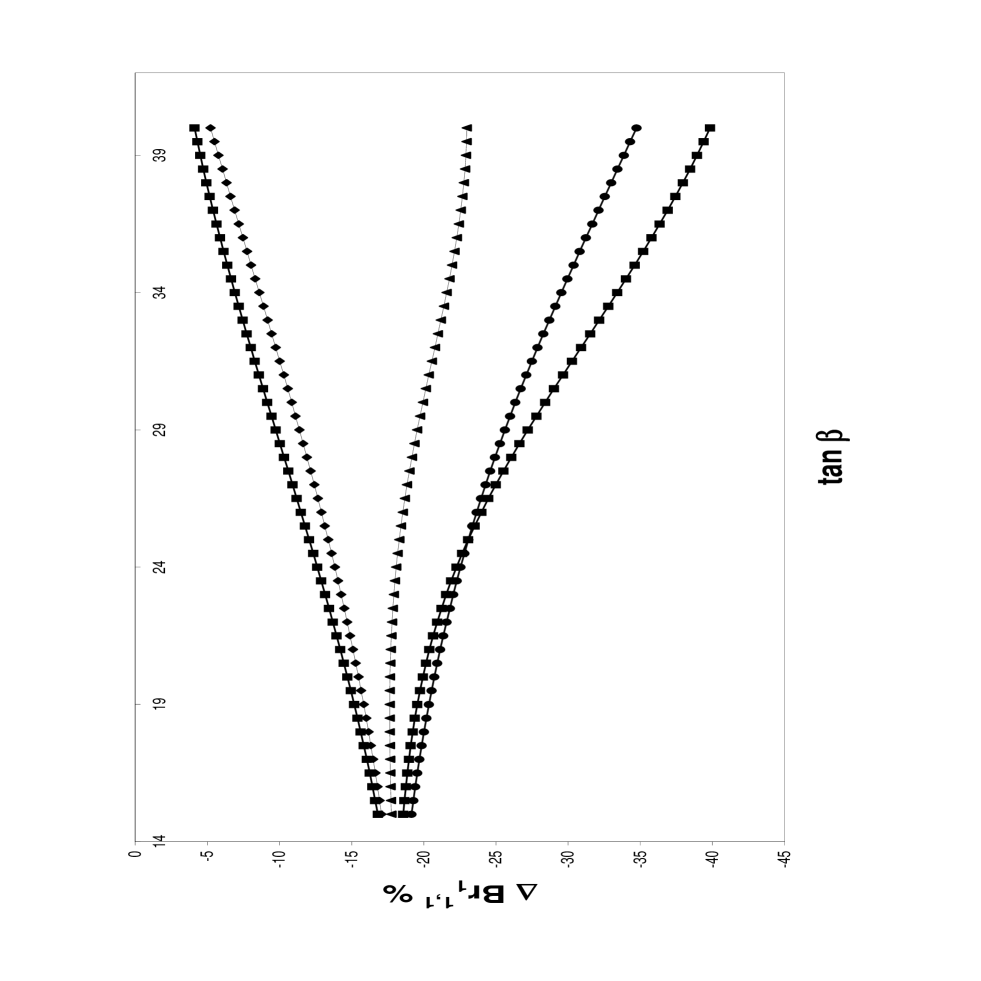
Figure 5: $\tan\beta$ dependence of $\Delta Br_{1}\to\chi_{1}^{+}\chi_{1}^{-}$. The curves in ascending order at $\tan\beta=40$ correspond to $\theta_{\mu}=0.5$, $0.1$, $1.0$, $1.5$ and $2.0$ (rad). The input is $m_{0}=500$ GeV, $m_{1/2}=150$ GeV, $\xi_{1}=0.4$ (rad), $\xi_{2}=0.5$ (rad), $\xi_{3}=0.6$ (rad), $\alpha_{A_{0}}=0.3$ (rad) and $|A_{0}|=250$ GeV.

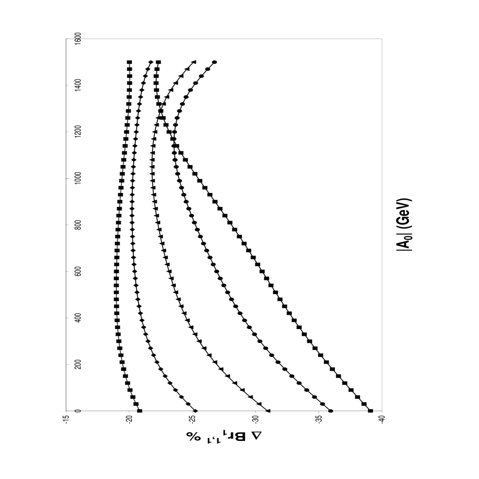
Figure 7: $|A_{0}|$ dependence of $\Delta Br_{1}\to\chi_{1}^{+}\chi_{1}^{-}$. The curves in ascending order at $|A_{0}|=0$ correspond to $\tan\beta=40$, $35$, $30$, $25$ and $20$. The input is $m_{0}=500$ GeV, $m_{1/2}=150$ GeV, $\xi_{1}=0.4$ (rad), $\xi_{2}=0.5$ (rad), $\xi_{3}=0.6$ (rad), $\theta_{\mu}=0.7$ (rad) and $\alpha_{A_{0}}=0.1$ (rad).

We investigate the question of how large loop corrections are relative to the tree values. We first discuss the magnitude of the loop corrections of the partial decay width defined in Eq.(52). As we mentioned earlier the loop corrections to the partial decay width of the chargino channel have been investigated before in the CP conserving case [20, 21]. The correction in these analyses is of the order of $\sim 10\%$ of the tree level value. Our analysis supports this conclusion. In Figs. (3) and (4) we give a plot of $\Delta\Gamma^{1,1}_{l}(l=1,3)$ as a function of $\tan\beta$ for the specific set of inputs given in the captions of these figures. We notice that the partial decay width gets a change of $7\sim 15\%$ of its tree level value. We also notice that the CP violating phase $\theta_{\mu}$ can affect the magnitude of this change. This effect has not been addressed in the previous analyses as they are working in the CP conserving scenario. To compare between our analysis and the previous ones we have to notice that these analyses are using the general SUSY parameter space where they put by hand all the parameters that control the analysis. In [20], the authors choose the SUSY parameter set SPS1a of the Snowmass Points and Slopes as a reference point. They choose for the trilinear couplings the values of $A_{t}=-487$ GeV, $A_{b}=-766$ GeV and $A_{\tau}=-250$ GeV. The values of the other parameters are: $M=197.6$ GeV, $M^{\prime}=98$ GeV, $\mu=353.1$ GeV, $\tan\beta=10$, $m_{A^{0}}=393.6$ GeV, $M_{\tilde{Q}_{1,2}}=558.9$ GeV, $M_{\tilde{U}_{1,2}}=540.5$ GeV, $M_{\tilde{D}_{1,2}}=538.5$ GeV, $M_{\tilde{L}_{1,2}}=197.9$ GeV, $M_{\tilde{E}_{1,2}}=137.8$ GeV, $M_{\tilde{Q}_{3}}=512.2$ GeV, $M_{\tilde{U}_{3}}=432.8$ GeV, $M_{\tilde{D}_{3}}=536.5$ GeV, $M_{\tilde{L}_{3}}=196.4$ GeV and $M_{\tilde{E}_{3}}=134.8$ GeV. In all the figures of [20], these values are used, if not specified otherwise. In our mSUGRA analysis the magnitude of all these parameters and others are fixed by the five input parameters $m_{0}=100$ GeV, $m_{1/2}=250$ GeV, $\tan\beta=10$, $A_{0}=-100$ GeV and a positive sign of $\mu$ in the CP conserving scenario [27]. These parameters are different from those of our Figs. (3) and (4). By using these parameters and fixing some of them by hand when needed to match their values in the analysis of [20], we were able to have a fair agreement with their Figs. (2-9). As an example of this check we show in Table.1 a comparison of the two works. For the input of Fig. 2 of [20] with CP violating phases are set to zero we can see that partial decay widths in both works have the same behavior as functions of masses and their magnitudes are fairly close to each other. However it seems that our loop corrected values of the partial widths are different from those of Eberl et al. This could be understood since our loop analysis of the effective lagrangian includes only the vertex corrections beside the corrections in the Higgs potential.

case	$\Gamma^{tree}_{eberl}$	$\Gamma^{tree}_{our}$	$\Gamma^{loop}_{eberl}$	$\Gamma^{loop}_{our}$
2.a $m_{A_{0}}=700$ GeV	$0.95$ GeV	$0.94$ GeV	$0.85$ GeV	$0.80$ GeV
2.a $m_{A_{0}}=800$ GeV	$1.18$ GeV	$1.17$ GeV	$1.0$ GeV	$0.91$ GeV
2.b $m_{H_{0}}=800$ GeV	$0.7$ GeV	$0.69$ GeV	$0.63$ GeV	$0.58$ GeV
2.b $m_{H_{0}}=900$ GeV	$0.8$ GeV	$0.8$ GeV	$0.73$ GeV	$0.70$ GeV

Table 1: A comparison between the current analysis and Eberl et al [20] for benchmark cases.

In the work of Ref. [21] only 8 out of 26 diagrams of the present analysis are calculated and they correspond to the vertex corrections from Figs. (1,2ii(a)), (1,2ii(b)), (1,2i(b)) and (1,2i(a)). By considering these diagrams only in the comparison, our analysis is in fair agreement with their Figs (2-4) and Figs. (6,8) for their inputs.

Now we turn to address the question of how much loop corrections can affect the branching ratios into charginos. The branching ratio of a decay mode is defined to be the ratio between the partial decay rate of this mode and the total decay rate. In the parameter space under investigation this total decay rate includes the rates of decays into charginos, heavy quarks, taus and neutralinos. In Figs. (5) and (6) we give a plot of $\Delta Br^{1,1}_{l}(l=1,3)$ defined by Eq.(53) as a function of $\tan\beta$ for the specific set of inputs given in the captions of these figures. Fig. (5) is for the neutral Higgs $H_{1}$ boson and Fig. (6) is for the neutral Higgs $H_{3}$ boson. In all regions of the parameter space investigated in this work, the decay of the lightest Higgs boson $H_{2}$ into charginos is forbidden kinematically, since we have in these regions the fact that $2m_{\chi^{-}_{1}}>m_{H_{2}}$. The analysis of Figs. (5) and (6) shows that the loop correction varies strongly with $\tan\beta$ with the correction changing sign for the case of $H_{3}$ decay. Further, the analysis shows that the loop correction can be as large as about $-40\%$ of the tree contribution for both $H_{1}$ and $H_{3}$ cases. We also notice that the behavior of $\Delta Br^{1,1}_{l}(l=1,3)$ as a function of $\tan\beta$ changes considerably by changing the phase of $\mu$. So for some values of this phase we find that this parameter increases as $\tan\beta$ increases and for other values of $\theta_{\mu}$ we see that it decreases as $\tan\beta$ increases. As shown in the previous figures, the parameter $\tan\beta$ is playing a strong role. This parameter is important at the tree level through the diagonalizing mass matrices of the chargino and neutral Higgs and their spectrum. At the loop level it has extra effect explicitly in $\alpha^{lP,S}_{jk}$ and implicitly through the radiatively corrected matrix elements $Y_{lm}$ and through the corrections $\delta\phi_{jk}$, $\Delta\phi_{jk}$, $\delta\psi_{jk}$, $\Delta\psi_{jk}$. The values of the branching ratios themselves at tree and one loop levels are shown in Table.2.

$\theta_{\mu}(rad)$	$Br^{0}(H_{1})$	$Br^{loop}(H_{1})$	$Br^{0}(H_{3})$	$Br^{loop}(H_{3})$
$0.5$	$6\%$	$4.7\%$	$18.2\%$	$13.8\%$
$1.0$	$8.4\%$	$6.9\%$	$21.3\%$	$18.1\%$
$1.5$	$9.2\%$	$7.9\%$	$23.4\%$	$22.2\%$

Table 2: Values of branching ratios at tree and one-loop levels of neutral Higgs into the channel $\chi^{+}_{1}\chi^{-}_{1}$ at $\tan\beta=24$ for the input of Figs. (5) and (6)

We notice that their magnitudes are not negligible for the region of the parameter space investigated. These non negligible branching ratios for the decay of the neutral Higgs into charginos suggest that these decay modes could be measurable at the soon-to-operate LHC. However, one should also consider the production rates for $H_{1}$ and $H_{3}$ bosons to assess whether the change in branching ratios could be detectable at colliders. This analysis goes beyond the scope of the current work. We also notice that the phase of the parameter $\mu$ affects the tree level branching ratios as well. This comes mainly from the structure of the chargino matrix. The more important channels in the region of the parameter space investigated are the decay into bottom and top quarks. They have the highest values of branching ratios. The radiative corrections of these channels are also more than those of the charginos and neutralinos. These channels were studied before [1, 15, 16] as mentioned above. However a $20\%$ of branching ratio for the case of neutral Higgs as shown in the above table is not very small and could justify carrying out the current analysis.

In Figs. (7) and (8) we give a plot of $\Delta Br^{1,1}_{l}(l=1,3)$ as a function of $|A_{0}|$ for the specific set of inputs given in the caption of these figures. The analysis of these figures shows that the loop corrections are substantial and reaches the value of $-38\%$ of the tree contribution for the case of $H_{1}$ decay and the value of $-43\%$ for the case of $H_{3}$ decay.

Next we investigate the effects of CP violating phases on the loop corrections of the neutral Higgs decays into charginos. In Figs. (9) and (10) we give a plot of $\Delta Br^{1,1}_{l}(l=1,3)$ as a function of $\theta_{\mu}$ for the specific set of inputs given in the caption of these figures. The analysis of the figures shows that the loop correction has a sharp dependence on $\theta_{\mu}$. Further, the correction is changing sign as $\theta_{\mu}$ varies from $0$ to $\pi$ for two cases of $H_{3}$ decay. Thus $\theta_{\mu}$ affects not only the magnitude of $\Delta Br^{1,1}_{l}$ but also its sign depending on the value of $\theta_{\mu}$.

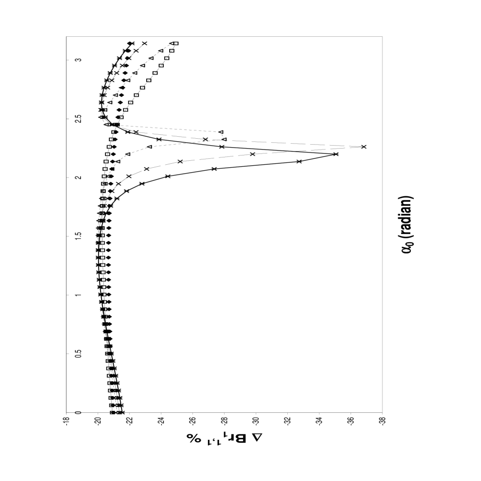
Figure 11: $\alpha_{0}$ dependence of $\Delta Br_{1}\to\chi_{1}^{+}\chi_{1}^{-}$. The curves in ascending order at $\alpha_{A_{0}}=2.2$ (rad) correspond to $|A_{0}|=500$, $450$, $400$, $100$ and $200$ GeV. The input is $\tan\beta=20.0$, $m_{0}=500$ GeV, $m_{1/2}=150$ GeV, $\xi_{1}=0.4$ (rad), $\xi_{2}=0.5$ (rad), $\xi_{3}=0.6$ (rad) and $\theta_{\mu}=0.1$ (rad).

In Figs. (11) and (12) we give a plot of $\Delta Br^{1,1}_{l}(l=1,3)$ as a function of $\alpha_{A_{0}}$ for the specific set of inputs given in the caption of these figures. Here also we find a very substantial dependence of $\Delta Br^{1,1}_{l}$ on $\alpha_{A_{0}}$. This dependence is very large in the case of $H_{3}$ decay and it exceeds $-40\%$ of the tree contribution.

In Figs. (13) and (14) we give a plot of $\Delta Br^{1,1}_{l}(l=1,3)$ as a function of $\xi_{2}$ for the specific set of inputs given in the caption of these figures. Here we find a small effect of this phase on the loop corrections.

5 CONCLUSION

In this paper we have carried out an analysis of the supersymmetric loop corrections to $\chi^{+}_{j}\chi^{-}_{k}H^{0}_{l}$ couplings within MSSM. In supersymmetry after spontaneous breaking of electroweak symmetry one is left with three neutral Higgs bosons which in the absence of CP phases consist of two CP even Higgs bosons and one CP odd Higgs boson. In the absence of loop corrections, the lightest Higgs boson mass satisfies the inequality $m_{h}<M_{Z}$ and by including these corrections the lightest Higgs mass can be lifted above $M_{Z}$. With the inclusion of CP phases the Higgs boson mass eigenstates are no longer CP even and CP odd states when loop corrections to the Higgs boson mass matrix are included. Further, inclusion of loop corrections to the couplings of charginos and neutral Higgs is in general dependent on CP phases. Thus the decays of neutral Higgs into charginos can be sensitive to the loop corrections and to the CP violating phases. The effect of the supersymmetric loop corrections is found to to be in the range of $7\sim 15\%$ for the partial decay width. For the branching ratios it is found to be be rather large, as much as $40\%$ in some regions of the parameter space. The effect of CP phases on the modifications of the partial decay width and the branching ratio is found to be substantial in some regions of the MSSM parameter space.

Acknowledgments
I wish to acknowledge useful discussions with Professor Pran Nath. The support of the Physics Department at Alexandria University is also acknowledged.

6 APPENDIX

The integral of import to this work is

$$J=\int\frac{d^{4}k}{(2\pi)^{4}}\frac{1}{(k^{2}-m^{2}_{1}+i\epsilon)(k^{2}-m^{2}_{2}+i\epsilon)(k^{2}-m^{2}_{3}+i\epsilon)}$$ (54)

It could be written in the form

$$\int\frac{d^{4}k}{(2\pi)^{4}}\frac{1}{D}$$ (55)

where

$$\frac{1}{D}=\frac{1}{a}\frac{1}{b}\frac{1}{c}$$

$$a=k^{2}-m^{2}_{1}+i\epsilon$$

$$b=k^{2}-m^{2}_{2}+i\epsilon$$

$$c=k^{2}-m^{2}_{3}+i\epsilon$$ (56)

Using Feynman parametrization, $\frac{1}{D}$ could be written as

$$\frac{1}{D}=2\int_{0}^{1}dx\int_{0}^{1-x}dz\frac{1}{[a+(b-a)x+(c-a)z]^{3}}$$ (57)

The denominator in the above integral could be written in the form $k^{2}+M^{2}+i\epsilon$ where $M^{2}=(m^{2}_{1}-m^{2}_{2})x+(m^{2}_{1}-m^{2}_{3})z-m^{2}_{1}$. Thus the integral $J$ can take the form

$$J=\int\frac{d^{4}k}{(2\pi)^{4}}2\int_{0}^{1}dx\int_{0}^{1-x}dz\frac{1}{[k^{2}+M^{2}+i\epsilon]^{3}}$$ (58)

Now integrating over $k$ and using the standard integral, for $n\geq 3$

$$\int\frac{d^{4}k}{(2\pi)^{4}}\frac{1}{(k^{2}+\Lambda+i\epsilon)^{n}}=i\pi^{2}\frac{\Gamma(n-2)}{\Gamma(n)}\frac{1}{\Lambda^{n-2}}$$ (59)

one can find that the integral $J$ has the form

$$J=\frac{i}{(4\pi)^{2}}\int_{0}^{1}dx\int_{0}^{1-x}dz\frac{1}{\alpha+\beta z}$$ (60)

where $\alpha=(m^{2}_{1}-m^{2}_{2})x-m^{2}_{1}$ and $\beta=m^{2}_{1}-m^{2}_{3}$. Integrating over $z$ one can get for the integral $J$ the form of

$$J=\frac{i}{(4\pi)^{2}}\frac{1}{m^{2}_{1}-m^{2}_{3}}\int_{0}^{1}dx\ln(\delta_{1}x-m^{2}_{3})-\ln(\delta_{2}x-m^{2}_{1})$$ (61)

where $\delta_{1}=m^{2}_{3}-m^{2}_{2}$ and $\delta_{2}=m^{2}_{1}-m^{2}_{2}$. Finally we integrate over $x$ to get for $J$ the form of

$$J=\frac{i}{(4\pi)^{2}}f(m^{2}_{1},m^{2}_{2},m^{2}_{3})$$ (62)

where

$$f(m^{2}_{1},m^{2}_{2},m^{2}_{3})=\frac{1}{m^{2}_{1}-m^{2}_{3}}\frac{1}{m^{2}_{3}-m^{2}_{2}}\frac{1}{m^{2}_{1}-m^{2}_{2}}$$

$$\times[m^{2}_{2}m^{2}_{3}\ln(\frac{m^{2}_{2}}{m^{2}_{3}})+m^{2}_{3}m^{2}_{1}\ln(\frac{m^{2}_{3}}{m^{2}_{1}})+m^{2}_{1}m^{2}_{2}\ln(\frac{m^{2}_{1}}{m^{2}_{2}})]$$ (63)

This is the famous form factor that appears in the analysis of the radiative corrections for the quark and lepton masses [28], the decay rates of neutral and charged Higgs into quarks and leptons [1, 15, 16, 18] and in the $b\rightarrow s\gamma$ process [17]. In the latter process, the authors are using different form factor $H(\frac{m^{2}_{1}}{m^{2}_{3}},\frac{m^{2}_{2}}{m^{2}_{3}})$. This form factor could be easily converted to our $f(m^{2}_{1},m^{2}_{2},m^{2}_{3})$ through the simple relation

$$m^{2}_{3}f(m^{2}_{1},m^{2}_{2},m^{2}_{3})=H(\frac{m^{2}_{1}}{m^{2}_{3}},\frac{m^{2}_{2}}{m^{2}_{3}})$$ (64)

For the case where two of the masses are equal, $m_{2}=m_{3}$, one can repeat the same analysis with $b=c=k^{2}-m^{2}_{3}+i\epsilon$ and $a=k^{2}-m^{2}_{1}+i\epsilon$. By doing so one can get for the form factor $J$

$$J=\frac{i}{(4\pi)^{2}}\frac{1}{(m^{2}_{3}-m^{2}_{1})^{2}}[m^{2}_{1}\ln(\frac{m^{2}_{3}}{m^{2}_{1}})+m^{2}_{1}-m^{2}_{3}]$$ (65)

Figure 1: Set of diagrams contributing to radiative corrections $\delta\phi_{jk}$ and $\Delta\psi_{jk}$. (i): (a) $s_{1}=\tilde{b}_{i}^{*}$, $s_{2}=\tilde{b}_{l}^{*}$, $f=t$; (b) $s_{1}=\tilde{t}_{i}$, $s_{2}=\tilde{t}_{l}$, $f=\bar{b}$; (c) $s_{1}=H^{+}$, $s_{2}=H^{+}$, $f=\chi^{0}_{i}$; (d) $s_{1}=H^{0}_{l}$, $s_{2}=H^{0}_{m}$, $f=\chi^{+}_{i}$; (e) $v_{1}=Z^{0}$, $v_{2}=Z^{0}$, $f=\chi^{+}_{i}$; (f) $v_{1}=W^{+}$, $v_{2}=W^{+}$, $f=\chi^{0}_{i}$. (ii): (a) $f_{1}=t$, $f_{2}=t$, $s=\tilde{b}_{i}^{*}$; (b) $f_{1}=\bar{b}$, $f_{2}=\bar{b}$, $s=\tilde{t}_{i}$; (c)$f_{1}=\chi^{0}_{i}$, $f_{2}=\chi^{0}_{l}$, $s=H^{+}$; (d) $f_{1}=\chi^{+}_{i}$, $f_{2}=\chi^{+}_{l}$, $s=H^{0}_{m}$; (e) $f_{1}=\chi^{+}_{i}$, $f_{2}=\chi^{+}_{l}$, $v=Z^{0}$; (f) $f_{1}=\chi^{0}_{i}$, $f_{2}=\chi^{0}_{l}$, $v=W$; (g) $f_{1}=\tau^{+}$, $f_{2}=\tau^{+}$, $s=\tilde{\nu}_{\tau}$.

Figure 3: $\tan\beta$ dependence of $\Delta\Gamma_{1}\to\chi_{1}^{+}\chi_{1}^{-}$. The curves in ascending order correspond to $\theta_{\mu}=0.2$, $0.4$, $0.6$ (rad). The input is $m_{0}=350$ GeV, $m_{1/2}=180$ GeV, $\xi_{1}=0.4$ (rad), $\xi_{2}=0.5$ (rad), $\xi_{3}=0.6$ (rad), $\alpha_{A_{0}}=0.8$ (rad) and $|A_{0}|=250$ GeV.

Figure 4: $\tan\beta$ dependence of $\Delta\Gamma_{3}\to\chi_{1}^{+}\chi_{1}^{-}$. The curves in ascending order correspond to $\theta_{\mu}=0.2$, $0.4$, $0.6$ (rad). The input is $m_{0}=350$ GeV, $m_{1/2}=180$ GeV, $\xi_{1}=0.4$ (rad), $\xi_{2}=0.5$ (rad), $\xi_{3}=0.6$ (rad), $\alpha_{A_{0}}=0.8$ (rad) and $|A_{0}|=250$ GeV.

Figure 6: $\tan\beta$ dependence of $\Delta Br_{3}\to\chi_{1}^{+}\chi_{1}^{-}$. The curves in ascending order at $\tan\beta=40$ correspond to $\theta_{\mu}=0.5$, $0.1$, $1.0$, $1.5$ and $2.0$(rad). The input is $m_{0}=500$ GeV, $m_{1/2}=150$ GeV, $\xi_{1}=0.4$ (rad), $\xi_{2}=0.5$ (rad), $\xi_{3}=0.6$ (rad), $\alpha_{A_{0}}=0.3$ (rad) and $|A_{0}|=250$ GeV.

Figure 8: $|A_{0}|$ dependence of $\Delta Br_{3}\to\chi_{1}^{+}\chi_{1}^{-}$. The curves in ascending order at $|A_{0}|=0$ correspond to $\tan\beta=40$, $35$, $30$, $25$ and $20$. The input is $m_{0}=500$ GeV, $m_{1/2}=150$ GeV, $\xi_{1}=0.4$ (rad), $\xi_{2}=0.5$ (rad), $\xi_{3}=0.6$ (rad), $\theta_{\mu}=0.7$ (rad) and $\alpha_{A_{0}}=0.1$ (rad).

Figure 9: $\theta_{\mu}$ dependence of $\Delta Br_{1}\to\chi_{1}^{+}\chi_{1}^{-}$. The curves in ascending order at $\theta_{\mu}=2.0$ (rad) correspond to $|A_{0}|=100$, $250$, $500$, $750$ and $900$ GeV. The input is $\tan\beta=20.0$, $m_{0}=500$ GeV, $m_{1/2}=150$ GeV, $\xi_{1}=0.4$ (rad), $\xi_{2}=0.5$ (rad), $\xi_{3}=0.6$ (rad) and $\alpha_{A_{0}}=0.2$ (rad).

Figure 10: $\theta_{\mu}$ dependence of $\Delta Br_{3}\to\chi_{1}^{+}\chi_{1}^{-}$. The curves in ascending order at $\theta_{\mu}=\pi$ (rad) correspond to $|A_{0}|=100$, $250$, $500$, $750$ and $900$ GeV. The input is $\tan\beta=20.0$, $m_{0}=500$ GeV, $m_{1/2}=150$ GeV, $\xi_{1}=0.4$ (rad), $\xi_{2}=0.5$ (rad), $\xi_{3}=0.6$ (rad) and $\alpha_{A_{0}}=0.2$ (rad).

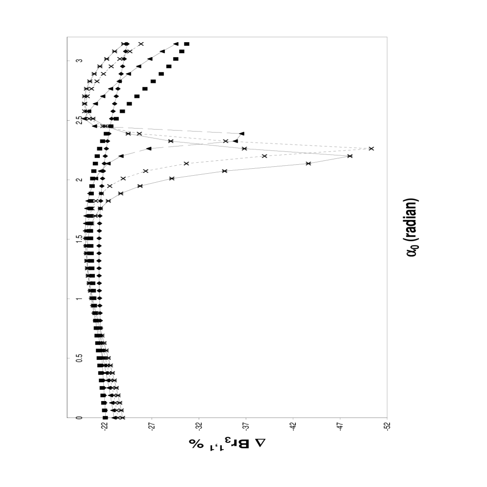
Figure 12: $\alpha_{0}$ dependence of $\Delta Br_{3}\to\chi_{1}^{+}\chi_{1}^{-}$. The curves in ascending order at $\alpha_{A_{0}}=2.2$ (rad) correspond to $|A_{0}|=500$, $450$, $400$, $100$ and $200$ GeV. The input is $\tan\beta=20.0$, $m_{0}=500$ GeV, $m_{1/2}=150$ GeV, $\xi_{1}=0.4$ (rad), $\xi_{2}=0.5$ (rad), $\xi_{3}=0.6$ (rad) and $\theta_{\mu}=0.1$ (rad).

Figure 13: $\xi_{2}$ dependence of $\Delta Br_{1}\to\chi_{1}^{+}\chi_{1}^{-}$. The curves in ascending order at $\xi_{2}=0.75$ (rad) correspond to $|A_{0}|=50$, $100$, $150$, $200$ and $250$ GeV. The input is $\tan\beta=20.0$, $m_{0}=500$ GeV, $m_{1/2}=150$ GeV, $\xi_{1}=0.4$ (rad), $\xi_{3}=0.6$ (rad) and $\theta_{\mu}=0.2$ (rad) and $\alpha_{A_{0}}=0.3$ (rad).

Figure 14: $\xi_{2}$ dependence of $\Delta Br_{3}\to\chi_{1}^{+}\chi_{1}^{-}$. The curves in ascending order at $\xi_{2}=0.75$ (rad) correspond to $|A_{0}|=50$, $100$, $150$, $200$ and $250$ GeV. The input is $\tan\beta=20.0$, $m_{0}=500$ GeV, $m_{1/2}=150$ GeV, $\xi_{1}=0.4$ (rad), $\xi_{3}=0.6$ (rad) and $\theta_{\mu}=0.2$ (rad) and $\alpha_{A_{0}}=0.3$ (rad).

References

- [1] M. Carena and H. e. Haber, Prog. Part. Nucl. Phys. 50, 63 (2003).
- [2] P. Nath, Phys. Rev. Lett.66, 2565(1991); Y. Kizukuri and N. Oshimo, Phys.Rev.D46,3025(1992). T. Ibrahim and P. Nath, Phys. Lett. B 418, 98 (1998); Phys. Rev. D57, 478(1998); Phys. Rev. D58, 111301(1998); T. Falk and K Olive, Phys. Lett. B 439, 71(1998); M. Brhlik, G.J. Good, and G.L. Kane, Phys. Rev. D59, 115004 (1999); A. Bartl, T. Gajdosik, W. Porod, P. Stockinger, and H. Stremnitzer, Phys. Rev. 60, 073003(1999); S. Pokorski, J. Rosiek and C.A. Savoy, Nucl.Phys. B570, 81(2000); E. Accomando, R. Arnowitt and B. Dutta, Phys. Rev. D 61, 115003 (2000); U. Chattopadhyay, T. Ibrahim, D.P. Roy, Phys.Rev.D64:013004,2001.
- [3] C. S. Huang and W. Liao, Phys. Rev. D 61, 116002 (2000); ibid, Phys. Rev. D 62, 016008 (2000); A.Bartl, T. Gajdosik, E.Lunghi, A. Masiero, W. Porod, H. Stremnitzer and O. Vives, hep-ph/0103324. M. Brhlik, L. Everett, G. Kane and J. Lykken, Phys. Rev. Lett. 83, 2124, 1999; Phys. Rev. D62, 035005(2000); E. Accomando, R. Arnowitt and B. Dutta, Phys. Rev. D61, 075010(2000); T. Ibrahim and P. Nath, Phys. Rev. D61, 093004(2000).
- [4] T. Falk, K.A. Olive, M. Prospelov, and R. Roiban, Nucl. Phys. B560, 3(1999); V. D. Barger, T. Falk, T. Han, J. Jiang, T. Li and T. Plehn, Phys. Rev. D 64, 056007 (2001); S.Abel, S. Khalil, O.Lebedev, Phys. Rev. Lett. 86, 5850(2001); T. Ibrahim and P. Nath, Phys. Rev. D 67, 016005 (2003) arXiv:hep-ph/0208142. D. Chang, W-Y.Keung,and A. Pilaftsis, Phys. Rev. Lett. 82, 900(1999).
- [5] E. Commins et al., Phys. Rev. A 50, 2960(1994)
- [6] P. G. Harris et al., Phys. Rev. Lett. 82, 904(1999)
- [7] S. K. Lamoreaux, J. P. Jacobs, B. R. Heckel, F. J. Raab, and E. N. Forston, Phys. Rev. Lett. 57, 3125(1986).
- [8] A. Pilaftsis, Phys. Rev. D58, 096010; Phys. Lett.B435, 88(1998); A. Pilaftsis and C.E.M. Wagner, Nucl. Phys. B553, 3(1999); D.A. Demir, Phys. Rev. D60, 055006(1999); S. Y. Choi, M. Drees and J. S. Lee, Phys. Lett. B 481, 57 (2000); T. Ibrahim, Phys. Rev. D 64, 035009 (2001).
- [9] S. W. Ham, S. K. Oh, E. J. Yoo, C. M. Kim and D. Son, arXiv:hep-ph/0205244; M. Boz, Mod. Phys. Lett. A 17, 215 (2002).
- [10] M. Carena, J. R. Ellis, A. Pilaftsis and C. E. Wagner, Nucl. Phys. B 625, 345 (2002) [arXiv:hep-ph/0111245]. J. Ellis, J. S. Lee and A. Pilaftsis, arXiv:hep-ph/0404167. E. Chrisova, H. Eberl, W. Majerotto, and S. Kraml, J. High Energy Phys. 12 (2002)021; E. Christova, H. Eberl, W. Majerotto, and S. Kraml, Nucl. Phys. B 639, 263(2002); 647, 359(E) (2002) T. Ibrahim, P. Nath, Phys and A. Psinas. Rev. D 70, 035006(2004).
- [11] U. Chattopadhyay, T. Ibrahim and P. Nath, Phys. Rev. D60,063505(1999); T. Falk, A. Ferstl and K. Olive, Astropart. Phys. 13, 301(2000); S. Khalil, Phys. Lett. B484, 98(2000); S. Khalil and Q. Shafi, Nucl.Phys. B564, 19(1999); K. Freese and P. Gondolo, hep-ph/9908390; S.Y. Choi, hep-ph/9908397; M. E. Gomez, T. Ibrahim, P. Nath and S. Skadhauge, Phys. Rev. D 70, 035014 (2004); T. Nihei and M. sasagawa, Phys. Rev. D 70, 055011(2004); 70, 079901(2004).
- [12] M. Gomez, T. Ibrahim, P. Nath and S. Skadhauge, Phys. Rev. D74, 015015(2006).
- [13] T. Ibrahim and P. Nath, hep-ph/0705.2008.
- [14] A. H. Chamseddine, R. Arnowitt, and P. nath, Phys. Rev. Lett. 49, 970(1982); R. Barbieri, S. Ferrara, and C. a. Savoy, Phys. Lett. B 119, 343(1982); L. Hall, J. Lykken, and S. weinberg, Phys. Rev. D 27, 2359(1983); P. Nath, R. Arnowitt, and A. H. Chamseddine, Nucl. Phys. B 227, 121(1983).
- [15] K. S. Babu and C. F. Kolda, Phys. Lett. B451, 77, 1999.
- [16] T. Ibrahim, P. Nath, Phys. Rev. D 68, 015008(2003).
- [17] D. A. Demir and K. A. Olive, Phs. Rev. 65, 034007 (2002); G. Degrassi, P. Gambino, and G. F. Giudice, J. High Energy Phys. 12, 009(2000); G. Belanger, F. Boudjema, A. Pukhov, and A. Semenov, Comput. Phys. Commun. 149, 103(2002).
- [18] T. Ibrahim, P. Nath, Phys. Rev. D 69, 075001(2004)
- [19] T. Ibrahim, P. Nath and A. Psinas, Phys. Rev. D 70, 035006(2004).
- [20] H. Eberl, W. Majerotto, Y. Yamada, Phys. Lett. B 597 (2004) 275.
- [21] Z. Ren-You, M. Wen-Gan, W. Lang-Hui and J. Yi, Phys. Rev. D 65, 075018(2002).
- [22] D. A. Demir, Phys. Rev. D 60, 055006(1999).
- [23] T. Ibrahim, P. Nath, Phys. Rev. D 63, 035009(2001).
- [24] T. Ibrahim, P. Nath, Phys. Rev. D 66, 015005(2002).
- [25] J. F. Gunion, H. E. Haber, Nucl. Phys. B 307, 445 (1988); A. Djouadi, hep/ph/9712334; A. Djouadi, J. Kalinowski, and M. Spira, Comp. Phys. Commun. 108, 56 (1998).
- [26] The neutralino decay of neutral Higgs with CP phases will be discussed elsewhere.
- [27] B. C. Allanach et al., Eur. Phys. J. C 25, 113 (2002).
- [28] M. Carena, M. Olechowski, S. Pokorski and C. E. M. Wagner, Nucl. Phys. B426 (1994) 269; L. J. Hall, R. Rattazzi and O. Sarid, Phys. Rev. D50 (1994) 7048; T. Ibrahim and P. Nath, Phys. Rev. D 67, 095003(2003).